Linear quantum optical bare raising operator

Linear quantum optical bare raising operator

Jennifer C. J. Radtke

E-mail: [email protected]

Daniel K. L. Oi

John Jeffers

SUPA Department of Physics, University of Strathclyde, Glasgow G4 0NG, UK

Abstract. We propose a simple implementation of the bare raising operator on coherent states via conditional measurement, which succeeds with high probability and fidelity. This operation works well not only on states with a Poissonian photon number distribution but also for a much wider class of states. As a part of this scheme, we highlight an experimentally testable effect in which a single photon is induced through a highly reflecting beamsplitter by a large amplitude coherent state, with probability 1/e(≈37%) in the limit of large coherent state amplitude.

1. Introduction

Operations on quantum states of light have a wide range of applications in quantum information processing and communication [1], as well as being of fundamental interest [2]. However, the operations that are easily implemented are limited to the class of Gaussian or linear operations [1]. Conditional evolution overcomes this limitation and provides a richer set of operations useful for manipulating continuous variable systems [3, 4, 5, 6]. Here, we show how to mimic the application of the bare raising operator to coherent state inputs using a beamsplitter, a single photon source, and a detector. In doing so we exploit a process that we call the quantum carburettor effect, whereby a strong coherent beam entrains the passage of a single photon (from an independent source) through a highly reflective beamsplitter with high probability, thereby elegantly highlighting the bosonic nature of light.

Conditional measurement-based evolution is a useful tool in discrete variable systems, such as the scheme by Knill, Laflamme and Milburn for efficient linear optical computing [7]. Discrete systems have been extensively studied [8], but have limitations particularly apparent in communications, where loss may be significant. Continuous variable schemes show greater promise here [1], but while Gaussian states such as coherent or squeezed states are relatively well understood, non-Gaussian states and operations have been less well-studied [9]. Non-Gaussian operations are required for tasks such as entanglement distillation and error correction, essential to the use of continuous variables in information processing protocols. In the continuous variable regime conditional evolution allows non-Gaussian operations [1]. There has significant interest in this approach [10, 12, 13, 11, 14, 15, 16], as the alternative of using nonlinear optics typically succeeds with low probability due to the weakness of nonlinear susceptibilities. Operations based on conditional measurement can be concatenated and this can allow operations which would not be possible deterministically, such as probabilistic state amplification [17, 18, 19, 20, 21, 22, 23, 24]. Here we look at a different way to increase the energy of a quantum state, by implementing the ladder or bare raising operator [25].

0.00 0.05 0.10 0.15 0.20 0.25 0.30 0.35 0.40

4 0 1 2 3

P

op

u

lat

ion

Photon number (a)

4 0 1 2 3

(b)

4 0 1 2 3

(c)

Figure 1. Comparison of the action of ˆa† and ˆE+ _{on a coherent state |αi,}

withα= 1. Figure shows Fock basis populations for: (a)|αi, (b) ˆa†|αi(after normalization) and (c) ˆE+_{|αi. Note that ˆa}† _{increases the relative probability} of higher excitation numbers (bosonic enhancement), whereas ˆE+ preserves the relative populations.

2. The bare raising operator

The bare raising and lowering operators, sometimes known as the Susskind-Glogower operators [25], act on the space of harmonic oscillator energy eigenstates to shift the amplitudes of a state of a system up or down the ladder by exactly one quantum without modifying their relative amplitudes. They are

ˆ E+=

∞

X

n=0

|n+ 1_ihn_|, Eˆ−=

∞

X

n=1

|n₋1_ihn_|, (1)

with ˆE+ = ( ˆE−)†. Note that while ˆE−Eˆ+ =1, ˆE+Eˆ− =1− |0ih0|, because acting with ˆE− _{on the ground state has no support. Unlike the more usual creation and}

annihilation operators ˆa† ₌P∞ n=0

√

n+ 1_|n+ 1_ihn_| and ˆa=P∞ n=1

√_n

|n₋1_ihn_| the bare operators do not introduce√nbosonic enhancement factors, as shown in figure 1. The corresponding operations are identical in their actions on a Fock state, but for a superposition or mixture of Fock states the difference between these two operations can be clearly seen. ˆE+ _{only shifts the Fock basis amplitudes up to a higher photon} number, whereas after normalization ˆa† _{increases the amplitudes of larger Fock states}

relative to lower ones. Therefore the bare raising and lowering operators can be used to shift the Fock state amplitudes of a quantum state up or down whilst preserving coherence, with the obvious exception of the ground state information being lost when the state is lowered.

t1 t2 t3 tn−1

0 0 0 0

|1_{i |}N_i

|1_{i |}1_{i |}1_{i |}1_i

Figure 2. Setup of scheme from figure 2 of [27] (redrawn) for the synthesis of large Fock states. The scheme succeeds when all detectors have no counts. The beamsplitters each have a different transmission probability to optimize the probability of a success, given success of the previous stage.

A scheme to synthesize arbitrary Fock states using beamsplitters and conditional measurement with single photon inputs was considered in 2005 by Escheret. al. [27] . Their system consisted of a cascade of beamsplitters, each combining a single photon Fock state with the output of the previous beamsplitter. This is depicted in figure 2. The scheme requiresN single photons to make a Fock state|Ni, and succeeds when all N −1 perfectly efficient detectors do not fire. They found that the maximum probability of a given detector not firing to be

P(0) =

_n

n+ 1

n

(2)

for a Fock state_|n_iand single photon input, leading to a_|n+ 1_ioutput. This occurs with a beamsplitter of transmission coefficient

tn = r

n

n+ 1 . (3)

Another similar scheme, again with cascaded beamsplitters and detectors, was considered in [31] for state preparation from single photons and coherent states. Both [31] and [27] simply considered implementing state preparation.

The standard creation operator ˆa† _{can be implemented approximately, either}

using postselected spontaneous parametric down conversion [32], or using a beamsplitter, single photon and detector. We use the latter approach here, but we aim to implement the bare raising operator ˆE+

|n_i=_|n+ 1_iinstead. The bare raising operator can be implemented in a two-stage process using attenuation followed by a creation operator [33]. Here we seek a one-stage linear optical implementation with corresponding high success probability and fidelity that works well on Gaussian states. We do this by an appropriate choice of the parameters of the single beamsplitter. One could also consider using existing implementations of ˆa† _{to approximate ˆE}+_{. For} simplicity, we use the ideal creation operator to make this comparison with our results. As ˆE+ _{is a trace preserving operation it can in principle be implemented} deterministically, unlike ˆa†. Recently, experimental implementations of ˆE+ _using cavity QED [34] or circuit QED [35] have been proposed that are in some cases deterministic and may allow practical applications. There is also a proposed implementation of ˆE−_{[36]. Linear optical nondeterministic implementations of}

3. Implementation ofEˆ+ _{with a single beamsplitter}

Physical implementations of non-Gaussian quantum optical operations normally work imperfectly and only effectively on a limited support. At the very least they are constrained physically by the amount of energy available. It is typical to tailor an operation to work with high fidelity on a set of states of interest or in restricted experimental parameter regimes, which limits the success probability. For example, probabilistic amplification only works on states with limited photon number; photon subtraction using a beamsplitter and a detector only works well in the low reflectivity limit. We take this standard approach: we optimise our operation for coherent states and find surprisingly that it works almost as well for a broad set of states of similar support.

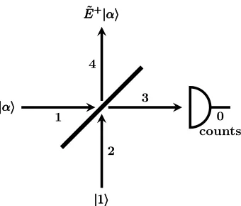
3.1. Setup

|_||ααα_iii

1

|||111_ii_i

2 3 4

˜ E+

|α_i ˜ E+

|α_i ˜ E+

|α_i

0 counts

Figure 3. Setup of scheme to implement ˆE+. A coherent state in mode 1 and a single photon in mode 2 are the inputs. Measurement of no photocounts at a perfectly efficient detector in mode 3 gives an approximate implementation of ˆE+ on the input coherent state, denoted ˜E+|αiin mode 4. The beamsplitter has transmission coefficienttand reflection coefficientr.

The essential setup used throughout is shown in figure 3, with coherent state and single photon inputs and measurement in one output mode [37]. A coherent state of mean photon number|α|2_{can be written as:}

|αi=e−|α|

2 2

∞

X

n=0 αn

√_n|ni , (4)

where_{|n_i}is the set of Fock states. The beamsplitter relations are

ˆ a†1 ˆ a†2

=

|t_|eiφT _−|r|e−iφR

|r_|eiφR _|t|e−iφT

ˆ a†3 ˆ a†4

, (5)

where_|t_|2₊

The joint input state to the beamsplitter is

|αi1|1i2=e

−|α|2 2 ∞ X n=0 αn √

n!|ni1|1i2≡

∞

X

n=0

qn|ni1|1i2 , (6)

whereqn =e

−|α|2

2 α

n √

n! (note that the following is also valid for any reasonable choice ofqn). This can be written in terms of the input mode creation operators acting on

the joint vacuum state:

|Ψin_i=

∞

X

n=0 qn

ˆ a†₁n

√

n!aˆ

†

2|00i12 . (7)

Application of the beamsplitter transformation in Eq. (5) gives the joint output as:

|Ψouti=

∞ X n=0 qn √ n!

|t|eiφT_ˆa†

3− |r|e−iφRaˆ†4

n

×|r_|eiφR_aˆ†

3+|t|e−i

φT_ˆa†

4

|00_i34 , (8)

which can be expanded to give:

|Ψouti =

∞ X n=0 n X k=0 qn √

n!(₋1)k

k!(n−k)!

×hA1

p

(n₋k+ 1)!k!_|n₋k+ 1_i3|k_i4

+A2

p

(n₋k)!(k+ 1)!_|n₋k_i3|k+ 1_i4i , (9)

where

A1=A1(n, k) =|t|n−k|r|k+1ei(n−k)φT−i(k−1)φR (10) A2=A2(n, k) =|t|n−k+1|r|kei(n−k−1)φT−ikφR . (11) After conditioning on no counts at the detector in mode 3 (i.e. k=n, 2nd term only), we find the normalized output is

˜

E+_|α_i= p1 P(0)

∞

X

n=0

qn|t||r|n

√

n+ 1_|n+ 1_i4 , (12)

where the success probabilityP(0) is given by

P(0) =

∞

X

n=0

|qn|2|t|2|r|2n(n+ 1) . (13)

Note that, in terms of a single mode, our beamsplitter-implemented operation may be expressed as ˜E+_=|t|ˆa†_|r|aˆ†_ˆa

3.2. Results

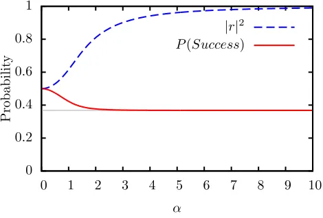
3.2.1. Perfect Detectors The most striking result is the behaviour of the success probability for the ˜E+ _{operation in the high n or α limit. The limit of Eq. (2)} as n _{→ ∞} is P(0) = 1/e for high-n Fock states. This result also holds for α _{→ ∞}, as shown numerically in figure 4. Thus a single photon is, with high probability, transmitted through a highly-reflecting mirror by an intense light beam. This “quantum carburettor”‡effect is not due to any coherence between the photon and the coherent state, as would be the case in a Mach-Zender interferometer for instance.

0 0.2 0.4 0.6 0.8 1

0 1 2 3 4 5 6 7 8 9 10

P

rob

ab

il

it

y

α

|r_|2 P(Success)

Figure 4. Success and reflection probabilities for the ˜E+ operation. The probability of no counts (red, solid) for the beamsplitter-implemented E˜+ operations for coherent state |αiinput is plotted, with limit 1/e (grey, solid), and the optimal value of the reflection probability|r|2_{(blue, dashed).}

The quantum carburettor effect can clearly be seen by the probability limit in figure 4. With a beamsplitter of the optimum reflection probability |ropt|2, the probability for the detection of zero photons with a perfect detector tends towards the limit 1/e _≈0.37. The optimum reflection probability tends towards a perfectly reflecting mirror, but even in this limit a single photon can be transmitted with probability 1/e if the appropriate amplitude coherent state is also incident on the beamsplitter.

We show the fidelity of the conditional output state after normalization with the ideal ˆE+

|α_i in figure 5, and also for comparison the fidelity of the state ˆa†_{|αi with}

the ideal ˆE+

|α_i. The different effect of ˆE+ _{and ˆa}† _{is clearest aroundα≈1, and the}

conditional output state has a much higher fidelity with ˆE+

|α_ithan the state ˆa†_|αi.

For sufficiently large _|α_|, the √n+ 1 term of equation (12) is approximately constant across the relevant Fock subspace that encompasses the majority of the support of the state, leading to the increased fidelity compared with lower |α|. Numerical results indicate that the reflection probability|ropt|2 for implementing the

ˆ

E+ _{operation with the highest fidelity coincides closely with that for the highest} success probability for large values of|α|(α >≈2.5).

0.94 0.95 0.96 0.97 0.98 0.99 1

0 1 2 3 4 5 6 7

F

id

el

it

y

α

Fidelity ˆE+ Fidelity ˆa† Fidelity ✶

Figure 5. Fidelities of the ˜E+operation and perfect ˆa†compared with the exact ˆ

E+ operation on coherent states. The fidelities of the normalized output state ˜

E+|αi (red, solid) and normalized ˆa†|αi (blue, dashed) are shown, compared to the ideal state Eˆ+|αi. The ‘do nothing’ fidelity of the original input coherent state with the ideal state is also shown (gray, dotted). Fidelities are

| hα|( ˆE+)†E˜+|αi |2_{, | hα|ˆaE}˜+_{|αi |}2 _{and | hα|( ˆE}+₎†|αi |2 _{respectively (with all}

states suitably normalized). The reflectivity of the beamsplitter was chosen to maximize the fidelity of the output state with ˆE+|αi.

To calculate the reflection probability corresponding to the maximum success probability, we differentiate Eq. (13) w.r.t. |r|2 _{and set equal to zero. Taking the} positive solution for|r|2 _{leads to}

|r_|2=|α|

2_{−3 +}p

|α|4_{+ 2|α|}2_{+ 5}

2_|α_|2 , (14)

which is valid above |α|2 _{= 0.5. Hence in the high |α| limit Eq. (14) is a good} approximation of the optimal reflection probability.

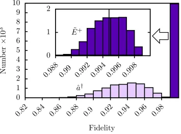
3.2.2. Arbitrary state inputs Although we tailor the beamsplitter reflection coefficient such that the operation works well for coherent states, the implementation is phase insensitive, so it works equally well for all states with Poissonian photon number statistics. Furthermore the operation also works well for states with a similar support to a coherent state. We illustrate this using randomly chosen states in a finite Fock basis. The inset of figure 6 shows the distribution of fidelities for a basis of up to 5 photons. An example state is shown in figure 7. All fidelities were greater than 0.988 and the mean fidelity was 0.99478. We also show that our operation is significantly different from the standard creation operator ˆa†_{by calculating the fidelity}

of approximating ˆE+ _{with ˆa}†_{, which is shown in the main part of figure 6 alongside}

the previous data. Despite our optimization for coherent states, our implementation of ˆE+ _{works well for a broad set of states, including randomly chosen states.}

0

1

2

3

4

5

6

7

8

9

10

0.

82

0.

84

0.

86

0.

88

0.

9

0.

92

0.

94

0.

96

0.

98

Nu

m

b

er

×

10

3

Fidelity

ˆ

a

0

1

2

0.

988

0.

99

0.

992

0.

994

0.

996

0.

998

˜

E

Figure 6.Distribution of the fidelities of ˆE+_{with the approximate ˜E}+_operation

(dark purple, main figure and inset) and ˆa† (light purple, main figure only) on random states. The inset shows the distribution of results in the far right hand bar of the main figure. 10,000 random states were generated using QuTiP’s rand ket function [38] with a maximum photon number of 6. The last element was set to 0 before renormalizing, to produce a state with random Fock state amplitudes in the range|0ito|5i. States were then operated on using our approximate ˜E+

operation with parameters optimised forα= 1.5 and the fidelity with the exact ˆ

E+ calculated after normalization. The mean fidelity was 0.99478 (marked by line on inset). The same states were also operated on with ˆa†for comparison.

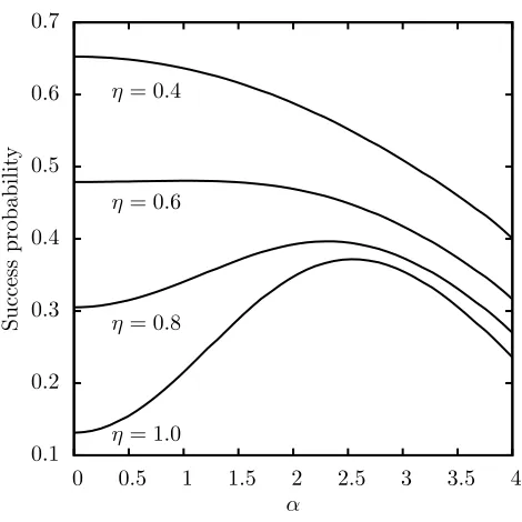
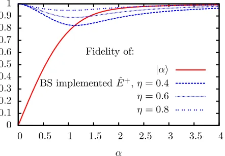
consideration for an experimental implementation would be the robustness to this detector inefficiency. This can be accounted for by using the normally ordered measurement operator : exp(−ηaˆ†aˆ) : in place of a simple projection [39, 6.10], where ηis the detector efficiency (the probability that a photon incident on the detector will be counted). Numerical calculations shown in figure 8 indicate that the model is not affected severely by the presence of moderate inefficiency. Numerical work was done in python with the aid of the QuTiP package [38].

0 0.1 0.2 0.3

0 1 2 3 4 5 6

P

op

u

lat

ion

Photon number (a)

0 1 2 3 4 5 6 (b)

Figure 7. An example implementation of (a) ˆE+|ψiand (b) the approximate ˜

E+|ψion a random state|ψifrom the set in figure 6. The fidelity is 0.9971.

0.1 0.2 0.3 0.4 0.5 0.6 0.7

0 0.5 1 1.5 2 2.5 3 3.5 4 η= 1.0

η= 0.8 η= 0.6 η= 0.4

S

u

cc

es

s

p

rob

ab

il

it

y

α

Figure 8.Effect of detector efficiency on ˜E+_{success probability. The probability}

of zero photocounts is plotted against α for fixed reflection probability |r|2 ₌

0 0.1 0.2 0.3 0.4 0.5 0.6 0.7 0.8 0.9 1

0 0.5 1 1.5 2 2.5 3 3.5 4 α

Fidelity of:

|α_i BS implemented ˆE+,η= 0.4 η= 0.6 η= 0.8

Figure 9. Comparison of the ˜E+ scheme with doing nothing when detectors are inefficient. The fidelity of the original coherent state|αiwith its photon number raised state ˆE+|αi (red,solid) and the fidelity of the normalized beamsplitter operation with ˆE+|αi are shown for values of the detector inefficiency η = 0.8,0.6,0.4 from top to bottom (blue, dashed). The crossing points indicate the discontinuity in the optimal reflection probability; at that point, it becomes more advantageous to simply reflect the input state rather than attempt an operation on it.

the point at which the ‘do nothing’ fidelity exceeds the achievable fidelity with the current set up. Note that for η > 1₋1/e _≈63% the ‘do nothing’ fidelity does not exceed the fidelity of our operation, and our operation produces a state with sub-poissonian variance which is non-classical even for large values of α. This detector efficiency is experimentally realistic – for instance, transition-edge sensors (TES) can offer efficiencies up to 98% [41].

3.2.4. Imperfect single photon sources Another significant experimental considera-tion is the producconsidera-tion of single photons. Here we briefly consider two imperfecconsidera-tions that may occur in single photon sources. Firstly we examine probabilistic sources that produce photons with a probabilityp, and vacuum otherwise. Secondly we consider heralded sources that produce pairs of single photons (one of which is measured to indicate the presence of the other), which occasionally produce instead pairs of the form_|2_{i |}2_i.

In the first case, it is still straightforward to observe the quantum carburettor effect. The single photon source outputs the state p_|1_{i h}1_|+ (1₋p)_|0_{i h}0_|. We can associate count ratesC1 and C0 for the single photon and vacuum contributions respectively. The overall observed count rate is then

Cobs=pC1+ (1−p)C0. (15)

0 0.05 0.1 0.15 0.2 0.25 0.3 0.35 0.4

0.98 0.985 0.99 0.995 1 1.005 1.01

P

rob

ab

il

it

y

|r_|2_/

|ropt|2

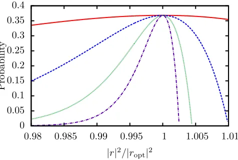
Figure 10. Probability of success with variation from the optimal beamsplitter reflectivity|ropt|2. This is for large values ofα: α= 5 (red, solid),α= 10 (blue,

dashed),α= 15 (green, dotted) andα= 20 (purple, dot-dashed). In each case the reflection probability has been normalised by the optimal reflection probability for thatα.

output then relies on the relative probabilities of these occurring, and can be expressed as

Ftotal=pF1+ (1−p)F0, (16)

noting that for highαinput the probability of detecting zero counts in either case is approximately equal. We can see that the fidelity achievable will be bounded below

bypF1, in the case that F1= 0 (which is a very pessimistic assumption).

In the second case, the two-photon rate is typically much lower than the one-photon rate. Our scheme reduces the impact of these states further, as at the optimal beamsplitter reflection probability the probabilityP(0) of obtaining 0 counts is reduced by approximately half for a 2 photon input compared to a single photon input.

3.2.5. Tolerance of variation in r At higher values of α, the success probability is very sensitive to variation in_|r_|2_{. This can be seen clearly in figure 10, which shows} the probability of success for fixed values ofα. This will impose some experimental limitation on the magnitude of α depending on the tolerances of the beamsplitter construction. Numerical results in figure 10 indicate that the drop off in success probability is slower for_|r_|<_|ropt|, as might be expected for the very high reflectivity required. It should be noted that the fidelity in this range is not significantly affected by changes in_|r_|2_{, only the probability of success.}

|α_i

|α_i

|α_i

1

|1_i

|1_i

|1_i

2 3 4

D1

x= 0,1 x= 0,1 x= 0,1 or>>>111

count(s) BS1

BS2

|1i |1_i

|1i

6

Switch

5

Ifx >1

Fail

Ifx= 1

8

|ψ2i

|ψ2i

|ψ2i

7

0 counts D2

Feedforward x Ifx= 0

|ψ1i

|ψ1i

|ψ1i

Figure 11. Cascaded ˜E+ _{operation. The lower beamsplitter (BS1), modes 1}

to 4, is as in the previous section. If a failure occurs at BS1, heralded by the single photocount at detector D1, the scheme now continues. The failed state from mode 4 is input into the upper beamsplitter (BS2) through mode 5, with a second ancilla single photon in mode 6, and a second attempt made to implement

˜

E+_{, with result|ψ2ioutput in mode 8 in the event that no photocounts occur at}

detector D2.

4. Cascaded Operation

With a more elaborate approach, it may be possible to improve on the scheme in the previous section. Here we consider a straightforward extension of the implementation of ˆE+_{, with extra components to correct a failed operation.}

4.1. Setup

The operation fails with 1 or more photocounts in mode 3. For the case of 1 count, we attempt the operation again on the failed output. This requires feedforward from the first detector, and an additional single photon, beamsplitter and detector as in figure 11. Figure 12 shows the possible measurement results at each detector, with their associated outcomes and probabilities. This may improve the success probability of the operation.

D1 Result

Accept FidelityFFF111

Fail

Retry

D2 Result

Accept

FidelityFFF222 Fail P1(0)

PP1(0)1(0)

PPP11(1((>>>1)1)1) P1(1) P1(1) P1(1)

P2(0)

PP2(0)2(0) _{PPP2(2(2(>>>0)0)0)}

Figure 12. Probability tree associated with the correction scheme in figure 11. D1 and D2 refer to the detectors as labelled in figure 11, whilePj(0) indicates the

no-count probability at thejth detector, andPj(1) the single-count probability.

If more than 1 count occurs, we do not attempt correction.

as before. If there is a count, a correction is attempted. When there is no count at detector 2 the correction is accepted and the unnormalized output state_|ψ2iin mode 8 is

∞

X

n=0

qn|r1|n−1(n|t1|2− |r1|2)|t2||r2|n√n+ 1|n+ 1i8 , (17)

where subscript 1 refers to the first beamsplitter parameters and 2 to the second. The normalization gives the probability of an initial failure (1 count at detector 1) and then an accepted correction (no counts at detector 2).

The fidelity measure used is the mean fidelity of accepted output states:

Fmean=

P1(0)F1+P1(1)P2(0)F2

P1(0) +P1(1)P2(0) , (18)

wherePj(0) indicates zero counts at thejth detector and therefore an accepted output

state at the relevant beamsplitter,Pj(1) indicates one photocount with the possibility

to correct the state, andFj is the fidelity of that state. The total success probability

is simplyP1(0) +P1(1)P2(0).

4.2. Results

Figure 13 shows, for various input |αi, the possible mean fidelities against their probabilities. Points cover the full range of beamsplitter pairs, whilst the solid line indicates use of beamsplitter 1 alone. It can be seen that the best fidelity is obtained using a single beamsplitter. For lower α an increase in probability is possible, but this results in a large loss of fidelity. This indicates that the strategy delivers only marginal improvement at best.

0.2 0.4 0.6 0.8 1.0

F

id

el

it

y _{α= 1.0 α= 2.0}

0 0.2 0.4 0.6 0.8

0 0.2 0.4 0.6 0.8 α=√2

0.2 0.4 0.6 0.8 1.0 Probability

α= 3.0

Figure 13. The success probability-fidelity trade off. The mean fidelities of the accepted output states ˜E+_{|αi with ideal state ˆE}+_{|αi for α = 1,2,}√₂

and 3 are shown, against the probability of obtaining that outcome in a 2 beamsplitter setup. Points (purple, light) cover the full range of possible pairs of beamsplitters and indicate the accessible region of fidelities and probabilities using this approach. The line (black, bold) indicates outcomes solely using a single beamsplitter.

‘hole’ in the photon number distribution of a coherent state, an effect described by Escher et al [42] and depicted in figure 14. Asαincreases, the optimal beamsplitter reflection coefficient |ropt| for the ˆE+ operation on a coherent state tends towards the reflection coefficient required to create a hole around n =_|α_|2 _{found by Escher} et al. Figure 14 shows this effect for α = 2, with the optimal beamsplitter for the

ˆ

E+ _{operation. This lack of amplitude at}

|α_|2 _{severely impacts on the fidelity of any} attempted recovery; while any divergence from this _|ropt| in the first beamsplitter reduces the probability and fidelity of an initially successful operation. Hence, the attempt at correcting a failed operation is not particularly successful.

5. Discussion and conclusions

The application of ˆE+ _{makes coherent states nonclassical. This is clearly seen by} noting that ˆE+

|α_ihas no zero photon component, a sign of nonclassicality [40]. From the basic scheme (figure 3) using linear optics and conditioning on a measurement outcome, it is clear that our implementation provides an experimentally-viable, high probability non-Gaussian operation with potential applications in continuous variable quantum information processing tasks such as entanglement distillation.

0 0.05 0.1 0.15 0.2 0.25 0.3 0.35

0 2 4 6 8 10 12

P

op

u

lat

ion

Photon number

Figure 14. Output state after a failed operation with 1 count in mode 3 and a perfect detector. The input state was a coherent state of amplitudeα= 2.

to improve the other as is the case with implementations of ˆa†_{. We achieve high}

fidelity and good success probability on a broad range of states, including randomly chosen states. A more elaborate optical scheme may be able to improve the success probability, as ˆE+ _{is in principle deterministic, as demonstrated in a cavity QED} proposal [34].

To observe the quantum carburettor effect experimentally, the main components required are a single photon source and a mode-matched laser, a beamsplitter, and a photodetector. As the measurement is conditioned on zero photocounts, a non-photon-number-resolving detector is sufficient. A variable beamsplitter would allow the 1/e limit to be investigated, by using different values of r to obtain results as in figure 8 and noting the corresponding maximum probability of no counts at the detector for eachr.

Future work could consider other schemes to improve the success probability for ˆ

E+_{, or look at ways to implement other non-Gaussian operations. An interesting} direction would be to quantify the achievable non-Gaussianity for a given set of experimental components, possibly in a resource theory framework.

Acknowledgments

The authors acknowledge useful discussions with Brian Gerardot and Adetunmise Dada. J. C. J. Radtke acknowledges support from the EPSRC Doctoral Training Grant, University of Strathclyde.

[1] S. L. Braunstein and P. van Loock, Rev. Mod. Phys.77, 2 (2005).

[2] K. Kraus, States, Effects, and Operations Fundamental Notions of Quantum Theory, volume 190 ofLecture Notes in Physics, (Springer Berlin Heidelberg, Berlin, Heidelberg 1983). [3] M. Ban, J. Mod. Opt.43, 6 (1996).

[4] R. Filip, P. Marek and U. L. Andersen, Phys. Rev. A71, 4 (2005).

[5] C. Vitelli, N. Spagnolo, F. Sciarrino and F. De Martini, Phys. Rev. A82, 6 (2010). [6] M. Dakna, L. Kn¨oll and D.-G. Welsch, Opt. Commun.145, January (1998). [7] E. Knill, R. Laflamme and G. J. Milburn, Nature409, January (2001).

[8] M. Nielsen and I. Chuang, Quantum computation and quantum information, (Cambridge University Press, New York, 10th anniv edition 2010).

[10] J. Wenger, R. Tualle-Brouri and P. Grangier, Phys. Rev. Lett.92, 15 (2004). [11] E. Andersson, M. Curty, and I. Jex, Phys. Rev. A74, 2 (2006).

[12] J. G. Walker, Opt. Acta Int. J. Opt.33, 3 (1986).

[13] V. Parigi, A. Zavatta, M. Kim and M. Bellini, Science317, 5846 (2007). [14] D. T. Pegg, L. S. Phillips and S. M. Barnett, Phys. Rev. Lett.81, 8 (1998).

[15] M. Dakna, T. Anhut, T. Opatrn´y, L. Kn¨oll and D.-G. Welsch, Phys. Rev. A55, 4 (1997). [16] A. Ourjoumtsev, R. Tualle-Brouri, J. Laurat and P. Grangier, Science312, 5770 (2006). [17] T. C. Ralph and A. P. Lund, inProceedings of the Ninth International Conference on Quantum

Communication, Measurement, and Computing edited by A. Lvovsky (AIP, Melville, New York, 2009), p. 155.

[18] F. Ferreyrol, M. Barbieri, R. Blandino, S. Fossier, R. Tualle-Brouri and P. Grangier, Phys. Rev. Lett.104, 12 (2010).

[19] P. Marek and R. Filip, Phys. Rev. A81, 2 (2010).

[20] G. Y. Xiang, T. C. Ralph, A. P. Lund, N. Walk, and G. J. Pryde, Nat. Photonics 4, 316 (2010). [21] M. A. Usuga, C. R. Mueller, C. Wittmann, P. Marek, R. Filip, C. Marquardt, G. Leuchs and

U. L. Andersen, Nat. Phys.6, 10 (2010).

[22] A. Zavatta, J. Fiur´aˇsek, and M. Bellini, Nat. Photonics5, 52 (2011).

[23] E. Eleftheriadou, S. M. Barnett and J. Jeffers, Phys. Rev. Lett.111, 21 (2013).

[24] R. J. Donaldson, R. J. Collins, E. Eleftheriadou, S. M. Barnett, J. Jeffers, and G. S. Buller, Phys. Rev. Lett. 114, 12 (2015).

[25] L. Susskind and J. Glogower, Physics (College. Park. Md).1, 1 (1964). [26] J. Clausen, M. Dakna, L. Kn¨oll and D.-G. Welsch, J. Opt. B1(1999). [27] B. M. Escher, A. T. Avelar and B. Baseia, Phys. Rev. A72, 4 (2005).

[28] F. E. S. Steinhoff, M. C. De Oliveira, J. Sperling and W. Vogel, Phys. Rev. A89, 3 (2014). [29] X. Zou, J. Shu and G. Guo, Phys. Lett. A359, 2 (2006).

[30] V. Potoˇcek, F. M. Miatto, M. Mirhosseini, O. S. Magana-Loaiza, A. C. Liapis, D. K. L. Oi, R. W. Boyd and J. Jeffers, Phys. Rev. Lett.115, 16 (2015).

[31] M. Dakna, J. Clausen, L. Kn¨oll and D.-G. Welsch, Phys. Rev. A59, 1658 (1999). [32] J. Clausen, H. Hansen, L. Kn¨oll, J. Mlynek and D.-G. Welsch, Appl. Phys. B50(2001). [33] M. Miˇcuda, I. Straka, M. Mikov´a, M. Duˇsek, N. J. Cerf, J. Fiur´aˇsek, and M. Jeˇzek, Phys. Rev.

Lett.109, 1 (2012).

[34] D. K. L. Oi, V. Potoˇcek and J. Jeffers, Phys. Rev. Lett.110, 21 (2013).

[35] J. Joo, M. Elliott, D. K. L. Oi, E. Ginossar and T. P. Spiller, New J. Phys.18, 2 (2016). [36] L. C. G. Govia, E. J. Pritchett, S. T. Merkel, D. Pineau and F. K. Wilhelm, Phys. Rev. A86,

3 (2012).

[37] Note thattandrare reversed compared to reference [27].

[38] J. R. Johansson, P. D. Nation and F. Nori, Comput. Phys. Commun.184, 4 (2013).

[39] R. Loudon, The Quantum Theory of Light, Oxford University Press, New York, 3rd edition (2000).

[40] L. Mandel and E. Wolf,Optical Coherence and Quantum Optics, Cambridge University Press, Cambridge (1995).