City, University of London Institutional Repository
Citation
:
Bessler, W., Blake, D., Lückoff, P. and Tonks, I. (2014). Why Does Mutual Fund Performance Not Persist? The impact and interaction of fund flows and manager changes (PI-1009). London, UK: Pensions Institute.This is the published version of the paper.
This version of the publication may differ from the final published
version.
Permanent repository link:
http://openaccess.city.ac.uk/17359/Link to published version
:
PI-1009Copyright and reuse:
City Research Online aims to make research
outputs of City, University of London available to a wider audience.
Copyright and Moral Rights remain with the author(s) and/or copyright
holders. URLs from City Research Online may be freely distributed and
linked to.
City Research Online: http://openaccess.city.ac.uk/ [email protected]
DISCUSSION PAPER PI-1009
Why Does Mutual Fund Performance Not
Persist?
The Impact and Interaction of Fund Flows and
Manager Changes
Wolfgang Bessler, David Blake, Peter Lückoff and Ian
Tonks
May 2014
ISSN 1367-580X
The Pensions Institute
Cass Business School
City University London
106 Bunhill Row
London EC1Y 8TZ
UNITED KINGDOM
Why does mutual fund performance not persist?
The impact and interaction of fund flows and manager changes
Wolfgang Bessler, David Blake, Peter Lückoff and Ian Tonks*
Abstract
We explain the lack of long-term performance persistence by actively managed U.S. equity mutual funds in terms of two equilibrating mechanisms: fund flows and manager changes. We find that these mechanisms acting together affect the future performance of past outperforming (winner) funds and past underperforming (loser) funds. Fund flows in isolation have a significant effect on performance, whereas manager changes in isolation have only a limited effect. A combination of both fund flows and manager changes has a substantial impact on future fund performance. If neither of these equilibrating mechanisms is operating, winner funds continue to significantly outperform loser funds by 4.08 percentage points per annum. However, the difference between winner and loser funds declines to almost zero if the two mechanisms are acting together. We also document that managers of winner funds increase risk, while managers of loser funds reduce risk, although losers who are fired took more risk than losers who keep their jobs.
JEL Classification: G28, G29, G32.
Keywords: Mutual funds, performance persistence, fund flows, manager changes.
*
1
1. INTRODUCTION
It is widely recognized that equity mutual fund performance does not persist in the long
term, even though some studies indicate that short-term persistence exists.1 Two alternative
explanations for the lack of long-term persistence are fund flows (Berk and Green, 2004) and
manager changes (Khorana, 1996, 2001; Dangl, Wu and Zechner, 2008). In this paper, we
investigate how far these two “equilibrating mechanisms”2 explain mean reversion in mutual
fund performance and whether they interact as substitutes or complements. If they are
complements, then they should be more effective in preventing performance persistence when
operating together. If they are substitutes, then the incremental effect of one mechanism,
conditional on the other operating, should be close to zero. In fact, we find that the two
mechanisms act as complements for both past outperforming (winner) and past underperforming
(loser) funds, based on a sample of 6,207 actively managed U.S. equity mutual funds over the
period from 1992 to 2011. For both outperforming and underperforming funds we find that
manager changes reinforce the effect of fund flows and can explain the erosion of performance
persistence.
For winner funds, we find that those funds experiencing both of the equilibrating
mechanisms – having relatively high net inflows and a manager change – underperform those
winner funds in which neither mechanism operates by 0.19 percentage points per month (2.28
1
See, e.g., Hendricks, Patel, and Zeckhauser (1993), Carhart (1997) and Pastor and Stambaugh (2002) for long-term performance persistence and Bollen and Busse (2005), Busse and Irvine (2006) and Huij and Verbeek (2007) for short-term performance persistence. Busse, Goyal, and Wahal (2010) document a similar pattern for institutional funds.
2
2
percentage points per annum)3 on a risk-adjusted basis in the following year. We find that fund
flows are the dominant reason for the lack of superior long-term performance persistence
amongst winner funds. However, the two mechanisms are complementary, since, in
combination, manager changes and fund flows result in an additional deterioration of
performance. Further, we provide evidence that winner funds increase their risk exposure.
For loser funds, as predicted by Dangl et al. (2008), we also detect a strong interaction
effect between both mechanisms. Manager changes, interpreted as an “internal governance”
mechanism, and outflows, treated as an “external governance” mechanism, reinforce each other
and the combined effect is a 0.16 percentage points per month (1.92 percentage points per
annum) higher risk-adjusted performance for loser funds experiencing both forms of governance
relative to funds experiencing neither. Both mechanisms are rather weak when operating in
isolation. Thus, while winner funds suffer from fund inflows irrespective of what happens to the
manager, the performance of loser funds is only affected when both mechanisms operate
together. Further, we confirm the prediction in Dangl et al. (2008) that, prior to a manager
change, fund risk increases, but falls post-replacement.
We go on to examine the spread in subsequent 12-month performance between winner
and loser funds, and we identify an unconditional spread of 0.22 percentage points per month
(2.64 percentage points per annum) in alphas, similar to the results in Carhart (1997). By
conditioning only on winner and loser funds that do not experience either of the equilibrating
mechanisms, our results produce a highly significant winner-minus-loser spread of 0.34
percentage points per month (4.08 percentage points per annum) in the subsequent year. In
3
3
contrast, by conditioning on winner and loser funds experiencing both equilibrating
mechanisms, the corresponding spread narrows to an insignificant -0.02 percentage points per
month (-0.24 percentage points per annum), implying that the substantial difference in alphas of
1.71 percentage points per month (20.52 percentage points per annum) between winner and
loser funds in the portfolio formation period is completely eliminated in the evaluation period.
These results indicate that a combination of both fund flows and manager changes explain the
lack of performance persistence and the mean reversion in mutual fund performance. We find
that performance persists when funds are not exposed to at least one equilibrating mechanism.
The rest of the paper proceeds as follows. The next section presents a review of the
literature and our hypotheses. In section 3, we describe our data set and explain our research
methodology. Our results are discussed in section 4. Using ranked portfolio tests, we analyze
fund flows, manager changes and their interaction for winner and loser funds separately, and
then examine the spread in winner-loser performance, before finally undertaking robustness
checks, including a pooled regression approach. Section 5 concludes and discusses the
implications of our findings.
2. LITERATURE REVIEW AND HYPOTHESES DEVELOPMENT
Berk and Green (2004) argue that mutual fund market equilibrium is attained through fund
flows. These respond to past performance, but due to decreasing returns to scale in active fund
management, the growth in fund size of recent winner funds causes their performance to
deteriorate, while loser-fund performance benefits from withdrawals that force managers to
re-optimize their portfolios. Chen et al. (2004) and Yan (2008) find that transaction costs are
positively correlated with fund size and the degree of illiquidity of the investment strategy and
4
Green (2004) hypothesis. Although the finding that small funds outperform large funds is
consistent with decreasing returns to scale in fund management, differences in fund sizes are the
result of both external growth due to the inflows accumulated throughout a fund’s full history
since inception and internal growth due to differential performance. Consequently, we focus
only on the most recent year’s fund flows as a flow variable, rather than fund size, to analyze its
equilibrium effect. Sirri and Tufano (1998) and Lynch and Musto (2003) document that past
outperformance triggers large inflows, but that investors in poorly performing funds typically
fail to withdraw their investments. Explanations for such behavior include: the anticipation of a
strategy change by the incumbent manager, the firing of a poorly performing manager, a
disposition effect (Shefrin and Statman, 1985; Singal and Xu, 2011), and investor inertia (Berk
and Tonks, 2007).
Edelen (1999), Alexander, Cici, and Gibson (2007) and Dubofsky (2010) argue that
excessive inflows or outflows encourage liquidity-motivated rather than valuation-motivated
trading by the managers subject to these flows and induce immediate transaction costs, both of
which are detrimental to short-run fund performance. Rakowski (2010) reports that funds with
more volatile flows underperform those with less volatile flows, which implies that outflows can
be as harmful for future performance as inflows, a finding that is incompatible with Berk and
Green’s (2004) conjecture that underperforming funds benefit from withdrawals. Even worse,
large outflows result in liquidity-motivated fire sales which distort fund performance and
impose even higher costs on loser funds (Coval and Stafford, 2007). Thus, we anticipate
asymmetric effects of fund flows on loser funds and winner funds, and we analyze each group
5
Khorana (1996), Chevalier and Ellison (1999) and Gallagher and Nadarajah (2004)
document an inverse relationship between fund performance and manager changes. Star fund
managers can extract a larger share of the higher fee income by either moving to a larger fund
within the same organization or to another fund family (Hu, Hall, and Harvey, 2000). Moreover,
a successful manager anticipating that she will be unable to repeat her outstanding performance
in the future may decide to use her current favorable track record to find a higher-paid job with a
new fund management company. In this case, the decision to stay or to leave will be the result of
the manager’s own assessment of her investment skill. The winner fund that loses its star
manager will need to hire a new manager, presumably with lower skills. Therefore, we would
expect fund performance to deteriorate after the hiring of a new manager. Khorana (2001) finds
that a manager change in outperforming funds results in a deterioration in performance from an
annual 1.9 percent in the pre-replacement period to 0.4 percent in the third year after
replacement. Loser-fund managers, in contrast, may be demoted to run smaller funds in the
same family or fired after a sustained period of poor performance. Khorana (2001) reports that
the performance of recently underperforming funds improves if the manager is replaced, in
which case abnormal performance rises from an annual -2.40 percent to 0.50 percent in the third
year after replacement. Hence, manager changes appear to contribute towards rectifying
negative performance persistence.
Dangl et al. (2008) develop a theoretical model of the mutual fund industry in which
poorly performing managers are subject to both external governance through market discipline
with investors withdrawing funds, and internal governance in the form of manager replacement.
The new manager also tends to change the fund’s risk profile relative to her predecessor. For
6
portfolio risk pre-replacement, as the fund manager anticipating a termination of the
employment contract takes on more risk in the hope of getting lucky (Brown, Harlow and
Starks, 1996; Chevalier and Ellison, 1997). After the manager is replaced, the model predicts
subsequent capital inflows and a decrease in portfolio risk.
Qiu (2003) and Kempf, Ruenzi, and Thiele (2009) suggest that employment risk
concerns could lead to fund managers taking less risk, while Huang, Sialm, and Zhang (2011)
argue that as well as these agency incentives, there are other risk considerations, such as
unskilled managers making poor investment decisions and skilled managers taking advantage of
market timing opportunities. Further, behavioral factors may also affect risk shifting behavior.
Prospect theory (Kahneman and Tversky, 1979) suggests that successful fund managers will
become more risk averse. On the other hand, overconfidence has been recognized as influencing
the behavior of both retail investors (Odean, 1999; and Grinblatt and Keloharju, 2009) and
institutional investors (Ekholm and Pasternack, 2008; Puetz and Ruenzi, 2011; Bar, Kempf and
Ruenzi, 2011). Overconfidence can be explained by biased self-attrition, whereby individuals
update their beliefs about their own ability as being attributable to skill following good
outcomes, but due to bad luck after bad outcomes. They become more overconfident after good
past performance, but not less confident after bad past performance (Daniel, Hirshleifer, and
Subrahmanyam, 1998; Gervais and Odean, 2001).
There exist several reasons to believe that fund flows and manager changes are not
independent of each other. Both mechanisms will be triggered by past performance, and the
results of Khorana (2001) that manager changes affect future fund performance might, in part,
be attributable to the effect of contemporaneous fund flows. Thus, it is important to control for
7
new managers as compared with continuing managers. In order to investigate these interaction
effects in detail, we classify the fund flows and manager change mechanisms as being
substitutes if the performance impact of one mechanism is smaller when the other mechanism
operates simultaneously. Fund flows and manager changes are interpreted as being complements
if the performance impact of one mechanism is larger when it operates jointly with the other
mechanism. In those cases where the performance impact of each mechanism is the same,
irrespective of whether it operates separately from or in combination with the other mechanism,
the mechanisms will be classified as being independent of each other.
In the case of winner funds, fund flows and manager changes are potential substitutes
because if net inflows remain low despite superior past performance, the fund manager is in a
weaker position to negotiate an improved compensation package, increasing the likelihood of
her leaving.4 In contrast, if the fund is subject to high net inflows, the manager may decide to
stay and reap the benefits from a larger asset base and hence higher fees. Moreover, if investors
observe that the star manager has left, they may rationally anticipate that superior past
performance will be less of a predictor of future performance, resulting in a weaker relationship
between past performance and current fund flows in the case of a manager change. A further
reason for these mechanisms being substitutes is that a newly appointed fund manager is likely
to adjust the portfolio holdings towards her own preferred investment strategy. If large net
inflows occur at the same time, the manager could use these inflows efficiently to adjust the
portfolio weights and, by doing so, reduce the marginal negative performance impact of high net
inflows.
4
8
Based on the findings of Pollet and Wilson (2008) that fund managers scale up existing
holdings as a response to inflows, it should be the case that fund flows and manager changes are
complements among winner funds. Specifically, if managerial skill determines the number of
“best ideas” a manager is able to generate (Cohen, Polk and Silli, 2010) and the newly hired
manager has lower skills and hence fewer good ideas than the former manager, then the same
level of inflows will have a stronger impact on lowering the performance of winner funds with a
manager change than on those without.
Whether these mechanisms are substitutes or complements is an empirical question that
our data set allows us to investigate. We address the following hypotheses and questions about
the joint effects of fund flows and manager changes on the performance persistence of winner
funds:
y Fund flows: Investors chase past performance and future performance suffers from high
inflows, leading to stronger mean reversion for winner funds with higher net inflows.
y Manager changes: A fund manager who leaves a winner fund is replaced with a less
skilled manager, resulting in reduced performance and stronger mean reversion for
winner funds with a manager change.
y Interaction: Fund flows and manager changes, when occurring simultaneously, have
either magnifying (complement) or offsetting (substitute) effects.
y Risk changes: How does a winning fund manager adjust her subsequent risk exposure?
According to prospect theory, risk aversion increases in the domain of gains and risk is
9
subject to an overconfidence bias, risk will increase (Barber and Odean, 2001;
Scheinkman and Xiong, 2003; Puetz and Ruenzi, 2011).
With loser funds, the Dangl et al. (2008) model predicts that the internal (termination of
a manager contract) and external (investors withdraw funds) governance mechanisms are
potential substitutes. If the manager has been replaced, investors will no longer see any reason
to withdraw money and instead will remain invested, waiting for a performance reversal.
Similarly, if money has flowed out of the fund, the management company might decide that the
existing manager will be able to improve fund performance with the smaller asset base (Berk
and Green, 2004).
Alternatively, internal and external governance in loser funds could reinforce each other
and act as complements. If the market has reacted quickly to poor past performance, the
management company may fire a poorly performing manager in an attempt to stem outflows.
Furthermore, causality could be reversed: if the disposition effect explains why many investors
in poorly performing funds do not withdraw their investments, a manager replacement can serve
as an attention trigger. Once investors are aware of both the manager change and the
underperformance, they then start withdrawing funds.5 Cremers and Nair (2005) investigate the
interaction between internal and external control mechanisms in the context of corporate
governance, and examine performance differentials between companies where one or both of
these mechanisms are present. Their results have implications for the incentives and penalties
facing corporate managers from the two governance mechanisms. Our study has similar
implications for the incentives and penalties facing fund managers.
5
10
As with winner funds, whether these mechanisms for underperforming equity mutual
funds are substitutes or complements is an empirical question. We address the following
hypotheses and questions about the effects of fund flows and manager changes on performance
persistence of loser funds:
y Fund flows: Investors withdraw their money and performance improves as a result of a
smaller asset base, since managers can concentrate on the most profitable investment
opportunities and this leads to stronger mean reversion for loser funds with higher
outflows, although this effect will be dampened by any investor inertia and by the costs
of re-optimizing portfolios.
y Manager changes: The fund management company fires an underperforming fund
manager and performance improves under a newly appointed fund manager, leading to
stronger mean reversion for loser funds with a manager change.
y Interaction: External and internal governance mechanisms, when occurring
simultaneously, have either magnifying (complement) or offsetting (substitute) effects.
y Risk changes: Prior to manager replacement, fund risk increases and post-replacement
fund risk falls (Dangl et al., 2008), although Kempf et al. (2009) predict employment
risk concerns will lead to fund managers taking less risk.
Finally, these two sets of hypotheses for winner and loser fund acting jointly have
implications for the spread in performance persistence between winner and loser funds. Our
main hypothesis in the paper states that:
y In the absence of fund flows and manager changes, past winners will continue to
11
We predict that if both equilibrating mechanisms operate on winner and loser funds together,
then the spread between winner and loser funds’ subsequent performance will be narrower than
when these mechanisms are not present.
3. DATA AND RESEARCH METHODOLOGY
3.1. DATA
Our mutual fund sample from the Center for Research in Security Prices (CRSP) starts in 1992,
the first year for which reliable information on manager changes becomes available, and ends in
2011. We follow Pastor and Stambaugh (2002) and select only actively managed U.S. domestic
equity funds (see Appendix). We aggregate all share classes of the same fund and drop all
observations prior to the IPO date given by CRSP and funds without names in order to account
for a potential incubation bias (Evans, 2010). Our final sample consists of 6,207 funds that
existed at some time during the period from 1992 to 2011 for at least 12 consecutive months.
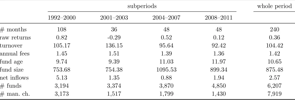
These funds have an average fund size of 875 million USD (Table 1). Fund size increased over
the sample period, whereas average fees fell from 1.45 percent to 1.36 percent of assets under
management, probably as a result of economies of scale in asset management.6
[Please insert Table 1 about here]
Monthly fund flows are constructed from the change in total net assets adjusted for internal
growth from investment returns:
(1) 1 ,
6
12
where TNAit refers to the total net assets of fund i at the end of period t and Rit is the return of
fund i between t-1 and t, assuming that all distributions are reinvested and are net of fund
expenses. On average, each fund received 2.57 million USD net inflows per month.
To obtain information on manager changes, we focus on the variable “mgr_date” in the
CRSP database, instead of using the specific names of the managers.7 This variable provides the
date of the last manager change as reported by the fund management company. By using the
manager date variable, we avoid any problems associated with different spellings of manager
names. Furthermore, as the number of team-managed funds increased during recent years, the
manager date variable has the advantage that fund management companies only report
significant changes in manager that are likely to have an impact on performance (Massa, Reuter,
and Zitzewitz, 2010). A total of 7,919 manager changes occurred during our sample period and,
on average, 15 percent of the fund managers are replaced each year.
3.2. RESEARCH METHODOLOGY
We use both ranked portfolio tests (Carhart, 1997; Carpenter and Lynch, 1999; Tonks, 2005)
and pooled regressions to investigate the hypotheses outlined in Section 2.
3.2.a. RANKED PORTFOLIO TESTS
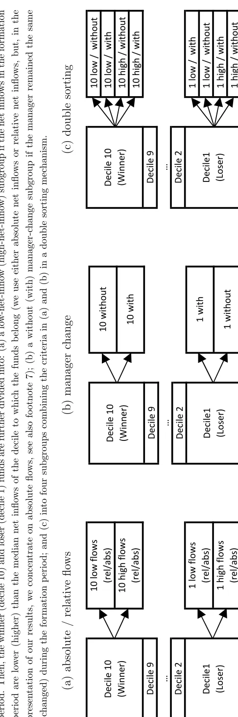
Funds are first ranked into equal-weighted decile portfolios based on their previous performance
over rolling twelve-month periods. Then, in a second sorting of the top-decile-10 and the
bottom-decile-1 portfolios, we form subgroups based on fund flows (low net inflows / high net
7
13
inflows) or manager changes (with manager change / without manager change), see Figure 1.8
Furthermore, as we are interested in the interaction effects between both mechanisms, we also
form subgroups by double sorting on fund flows and manager changes simultaneously (low with
/ low without / high with / high without). We analyze the performance of these subgroups of top
and bottom decile portfolios and the performance of spread portfolios in order to compare
alternative investment strategies.
[Please insert Figure 1 about here]
The decile portfolios are formed (a) on the basis of each fund’s alpha in the previous year or (b)
on the basis of previous year raw returns. For the first method, funds are ranked by alphas from
a Carhart (1997) four-factor model estimated over the previous 12 months (the formation
period), where the four common factors are the excess return above the risk-free rate on the
market index , the returns on a size factor , a book-to-market factor ( , and a
momentum factor ( ).9 Fund excess returns above the risk-free rate accounting for
different fund styles are given by:
(2)
8
In Berk and Green (2004), active management suffers from decreasing returns to scale, but it is an empirical question whether these capacity constraints are absolute or relative. Absolute capacity constraints arise once a certain threshold of absolute fund size is exceeded and depend on absolute fund flows. Relative capacity constraints differ across investment strategies and arise after the fund receives a certain level of inflows relative to the initial fund size. We analyze both absolute and relative net inflows, but, in the presentation of our results, we concentrate on absolute flows because the results for relative fund flows are qualitatively very similar though slightly weaker.
9
We also experimented with different five-factor model: first, a five-factor model that adds a mean reversion factor (based on six value-weighted portfolios formed on the size and prior returns of all NYSE, AMEX and NASDAQ
stocks, and downloaded from Kenneth French’s website: mba.tuck.dartmouth.edu/pages/faculty/ken.french/data_library.html) to the Carhart model: if winner funds hold on
14
To assess performance and fund flows in a timely manner, we focus on the previous
12-month horizon. Using such a short horizon to estimate alphas from a factor model is problematic
on account of the low degrees of freedom available for estimating (2). Nevertheless, we are able
to efficiently estimate (2) over this short horizon by applying the “empirical Bayesian”
adjustment procedure discussed in Huij and Verbeek (2007, hereafter HV), assuming a
multivariate normal prior. Let , , , , be a vector of unknown parameters to
be estimated. The cross-sectional distribution of the funds’ alphas and betas is assumed to be
normal, ~ ,Σ , where is a 5-dimensional vector of cross-sectional means of alphas and
betas, and Σ is a 5x5 covariance matrix. Assuming the errors in (2) are ~ 0, , the
posterior distribution of also is normal with expectation:
(3) Σ Σ
where is the matrix of returns on the four factors plus the intercept, is the OLS parameter
estimate, and is the variance of the errors in (2). The corresponding covariance matrix is
given by:
(4) Σ
As the prior mean µ and the prior covariance matrix Σ in eq. (3) and (4), we take the
cross-sectional averages of the time series OLS estimates of the coefficients of (2) and their
15
given 12-month formation period.10 Thus, we have the same priors for all funds in a given
month. According to eq. (3), the posterior estimate of is the matrix-weighted average of the
prior and the OLS estimate ; the same holds for the posterior estimate of the covariance
matrix in eq. (4).11. Confidence in the prior is the reciprocal of the estimation efficiency of the
OLS estimate for each fund. Thus, the empirical Bayesian adjustment ‘shrinks’ any extreme
parameters towards the mean of the prior, where the degree of shrinkage depends on the
cross-sectional dispersion of the parameters, given by Σ. The Bayesian adjustment is greater, the lower
the estimation efficiency of the funds' OLS parameters. The intuition is that it is less likely for a
fund to generate high alphas if all other funds generate relatively low alphas during the same
period. However, the posterior distribution of also takes the multivariate nature of the
coefficients’ dependency into account: e.g. if small-cap funds tend to have positive alphas (i.e.
there is a positive correlation between and in eq. (2)), a potentially negative OLS estimate
of a small-cap fund i’s alpha receives a positive adjustment by the Bayesian approach.
This argument is similar to the methodology of Cohen, Coval and Pastor (2005) who, in
addition, take the similarity in investment strategies into account. They attribute a higher skill
level to fund managers who deliver their outperformance with a similar strategy to other skilled
fund managers in comparison with managers who used a completely different strategy. The
latter are classified as lucky rather than skilled. Consequently, alpha-sorting based on Bayesian
10
Specifically, we estimate time-series OLS regressions for each of the N funds in the data set for months 1 to 12. We average the N estimates to form µ and use the empirical covariance matrix of these N estimates to form Σ. We plug µ and Σ into eq. (3) and (4) to obtain the mean and variance of the posterior distribution of for month 13. We repeat this process using the observations in months 2 to 13 in order to obtain the posterior distribution in month 14. We continue until the end of our data set using these rolling windows.
11
16
four-factor alphas accounts for a risk-adjustment of the performance measure used for the
ranking, corrects for different investment styles and reduces the influence of high-risk strategies
on the ranking. We also compare these results with portfolio formation based on raw returns, but
we believe that, in contrast to the raw return-sorting, the Bayesian alpha-sorting provides a
much more reliable separation between skilled and unskilled but lucky fund managers.12
3.2.b. REGRESSION
We also perform a pooled regression with the difference in annualized performance between the
evaluation year and the formation year as the dependent variable. These performance changes
over time are then regressed on a set of control variables, including net inflows and a manager
change dummy. This regression offers additional insights into the impact of fund flows and
manager changes on fund performance over time. Furthermore, it provides us with the
opportunity not only of separating the effects of fund flows and manager changes, but also of
measuring their marginal impact and their interaction with other fund characteristics.
4. EMPIRICAL RESULTS
4.1. PERFORMANCE PERSISTENCE
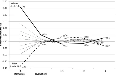
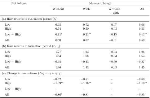
Figure 2 reveals that our results on the dynamics of mutual fund returns over time are consistent
with the earlier conclusions of Carhart (1997) who reported a lack of performance persistence
and a strong tendency for performance to mean revert. Specifically, the top ten percent of funds
(winner funds)13 generate raw returns in the formation year of 1.45 percent per month which
decline to 0.59 percent per month in the subsequent evaluation year. The bottom ten percent of
12
The average fund flows in the deciles and subgroups are not qualitatively different when we form portfolio deciles based on raw returns instead of the Bayesian four-factor alphas. One might conjecture raw returns are more relevant because retail investors are unlikely to calculate four-factor alphas. The subgroups should not be affected as we explicitly use fund flows as a second sorting mechanism.
13
17
funds (loser funds), in contrast, experience a mean reversion in raw returns from -0.36 to 0.34
percent per month. In other words, a raw return spread of 1.81 percent per month (21.72 percent
per annum) in the formation year declines to 0.25 percent per month (3.00 percent per annum) in
the evaluation year. Having established that performance persistence is mean reverting amongst
both winner funds and loser funds, we now investigate how fund flows and manager changes
affect these results.
[Please insert Figure 2 about here]
4.2. WINNER FUNDS
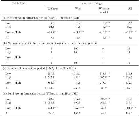
Winner funds, on average, have a formation-period fund size of 794.0 million USD, receive 8.5
million USD of new net inflows per month and the manager changes in 17 percent of the cases
(Table 2). They grow to an average size of 1,037.0 million USD in the evaluation period due to
internal (investment performance) and external growth (fund flows). Conditioning on fund
flows, we separate winner funds into a subgroup with “low absolute net inflows” during the
formation period averaging -5.6 million USD per month and a subgroup with “high absolute net
inflows” averaging 22.6 million USD per month, a significant difference of 28.2 million USD.
The fraction of managers leaving winner funds is the same for both subgroups at 17 percent, but
winner funds with low absolute net inflows tend to be smaller (675.0 million USD) than winner
funds with high absolute net inflows (976.4 million USD).14 Conditioning on manager changes
yields a subgroup “without manager change” which has slightly higher inflows and a larger
average fund size compared to the subgroup “with manager change” (Table 2, panel (c)).
14
18
[Please insert Table 2 about here]
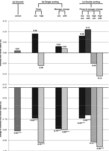
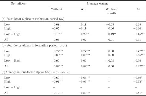
Winner Decile-10 funds, on average, generate alphas of 0.01 percent per month, equivalent to a
mean reversion from the formation to the evaluation period of -0.81 percentage points per
month (Table 3, panels (a) and (c), and Figure 3). Winner funds experiencing neither inflows
nor a manager change outperform the benchmark model (2) by 0.08 percentage points per
month, though this is not significantly different from zero. This corresponds to a significant
mean reversion of only -0.69 percentage points per month. Winner funds suffering from both
high inflows and a manager change generate negative, albeit insignificant, alphas of -0.11
percent per month, equivalent to a significant mean reversion of -0.96 percentage points per
month. The evaluation-period spread in alphas of 0.19 percentage points per month between
winner funds suffering from neither mechanism and those experiencing both is significant, both
in statistical and economic terms (0.19 = 0.08 (low/ without) – (-0.11) (high/ with), Table 3,
panel (a)). The difference in raw returns between winner funds suffering from both equilibrating
mechanisms and those affected by neither one is also striking: raw returns of the former revert to
equilibrium at -1.16 percentage points per month compared with -0.62 percentage points per
month for the latter (Table 4, panel (c)). We conclude from this that fund flows and manager
changes acting together strongly contribute to mean reversion in winner-fund performance.
[Please insert Tables 3 and 4 and Figure 3 about here]
As we have seen in Table 2, panel (b), the occurrence of a manager change seems to be
independent of fund flows, since, on average, 17 percent of managers change each year in both
subgroups with high and low net inflows. The difference in fund flows between winner funds
19
3.6 million USD. We conclude that the incidence of one mechanism does not affect the
likelihood of the other mechanism occurring.
Even though the occurrence of either mechanism appears to be independent, controlling
for one mechanism could still alter the impact of the other mechanism on future investment
performance. In fact, this is what we find. Among winner funds, there is evidence that the two
mechanisms interact as complements. If there is a manager change, fund inflows have a
significantly negative impact on performance of 0.22 percentage points per month, whereas if
there is no manager change, the differential effect of low and high fund inflows is only 0.13
percentage points per month (Table 3, panel (a)). When controlling for fund flows and
investigating the effects of a manager change, the spread in alphas is an insignificant -0.03
percentage points per month for the low-inflow subgroup, but a positive, though insignificant
0.06 percentage points per month for the high-inflow subgroup, in contrast with the case of a
manager change (Table 3, panel (a)). Comparing the single sorting results, fund flows have a
powerful effect on performance with the spread in alphas between the low inflows and high
inflows groups being a significant 0.15 percentage points per month. In contrast, a single sort on
the change in manager has little effect on the performance of these winner funds with only a
0.01 percentage points per month spread. We conclude that fund flows by themselves and also
in conjunction with manager changes significantly affect winner-fund performance and are
complementary to each other. High net inflows are more harmful for subsequent performance
than a manager change, possibly as a result of the transaction costs triggered by a
liquidity-induced increase in trading.
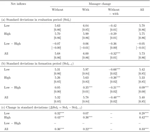
Finally for winner funds, we examine portfolio risk changes between the formation and
20
fund sub-group and the spread portfolios. In addition, the fractions of the standard deviation
explained by systemic risk according to the four-factor model (2), are reported in square
brackets underneath each standard deviation. Table 5, panel (c) shows that winner funds
significantly increase risk between the two periods by 0.33 percentage points per month
irrespective of whether there is a manager change or whether inflows are high or low. However,
the increase in risk is much larger (0.43 percentage points per month) if there is no manager
change and if the fund is experiencing high inflows. The increase in risk is much weaker (0.07
percentage points per month), and not statistically significant, in the case of a manager change
and low inflows. These findings are consistent with the presence of an overconfidence bias in
investment decision making by successful fund managers. Comparing the changes in these
systematic and idiosyncratic values between the formation and evaluation periods for each
portfolio, it can be seen that there are only very minor changes between the formation and
evaluation periods, so the changes in risk must be explained by both systematic and
idiosyncratic components (Table 5, panels (a) and (b)).
[Please insert Table 5 about here]
4.3. LOSER FUNDS
Loser funds, on average, are smaller compared with winner funds with total net assets of 700.4
million USD in the formation period (Table 6). Fund size remains relatively stable over time and
decreases only slightly to 681.0 million USD in the evaluation period. This is explained by net
inflows being negative, as expected, although small in magnitude at only -2.3 million USD per
month, on average. It is clear that many investors are reluctant to withdraw money from poorly
performing funds. We sort the loser-decile-1 funds into two subgroups on the basis of net
21
million USD and the other with high net inflows averaging 7.8 million USD. The difference in
average fund flows between the low- and high-fund-flow subgroups of loser funds is only about
two-thirds as large as the same difference for winner funds (20.2 million USD versus 28.2
million USD). Loser funds with high net inflows and a manager change are the smallest
subgroup in the formation period with a size of 374.1 million USD, while loser funds
experiencing both governance mechanisms simultaneously are the largest at 688.6 million USD
(Table 6, panel (c)).
[Please insert Table 6 about here]
Tables 7 and 8 report the interaction of the two governance mechanisms and fund performance
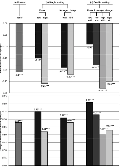
(see also Figure 4). Loser-fund performance, on average, reverts from alphas of -0.89 percent
per month in the formation period to a still significantly negative -0.21 percent per month in the
evaluation period, a statistically significant performance improvement of 0.68 percentage points
per month (Table 7, and Figure 4). However, distinct differences emerge in evaluation-period
performance when conditioning on both governance mechanisms. Loser funds that benefit from
both mechanisms have insignificant alphas of -0.09 percent per month in the evaluation period
compared with significant alphas of -0.90 percent per month in the formation period which
corresponds to a striking degree of mean reversion of 0.81 percentage points per month. Funds
without either form of governance mechanism continue to significantly underperform by -0.25
percentage points per month, regressing to the mean by only 0.63 percentage points per month.
The spread in alphas between loser funds experiencing both governance mechanisms and those
not benefiting from either is a highly significant 0.16 percentage points per month (0.16 = -0.09
22
raw returns are even more pronounced: the raw returns of loser funds with a manager
replacement and low net inflows improve by a (weakly) significant 0.84 percentage points per
month; while the raw returns of loser funds without a manager change and high net inflows
improve by an insignificant 0.56 percentage points per month (Table 8, panel (c)). Thus, if
operating simultaneously, the internal and external governance mechanisms strongly contribute
to an improvement in loser-fund performance.
[Please insert Tables 7 and 8 and Figure 4 about here]
How do both mechanisms contribute to this effect? A comparison of the characteristics
of the subgroups reveals that the internal and external governance mechanisms interact
positively: funds with low net inflows have a higher fraction of manager changes (22 percent)
than funds with high net inflows (16 percent) and funds with a manager change have lower net
inflows (-4.5 million USD per month) than funds without (-1.8 million USD per month)
(Table 6, panels (a) and (b)). Moreover, internal and external governance among loser funds are
also complements in terms of their performance impact. The alpha spread between loser funds
with low net inflows and those with high net inflows is significantly positive at 0.19 percentage
points per month only when internal governance is operating at the same time. If there is no
internal governance, this spread is a weakly significant 0.08 percentage points per month
(Table 7, panel (a)). Conversely, the spread between loser funds with a manager replacement
and those without is positive but insignificant at 0.08 percentage points per month if money is
flowing out of the fund at the same time, while it is negative and also insignificant at -0.03
percentage points per month if outflows do not occur. Also internal governance seems to be
23
The results for raw returns are similar though slightly smaller in magnitude, especially in
the case where both mechanisms are not operating simultaneously. In fact, outflows appear to
improve loser-fund raw returns by significant 0.21 percentage points per month in combination
with a manager replacement, although the low-minus-high raw-return spread is still a positive
but insignificant 0.08 percentage points per month in the case of no manager change (Table 8,
panel (a)). Compared with the similar sized alpha spread of the same subgroup, this implies that
fund managers who stay with the fund do not seem to use the outflows to re-optimize their
portfolio by bringing in new investment ideas, but merely scale down existing investments in a
way that reduces unfavorable factor loadings in the benchmark model. Specifically, loser funds
without outflows have significantly negative momentum loadings, while those experiencing
outflows reduce these loadings to levels close to zero (not reported in the tables).
We conclude from this that loser funds suffer from two types of disposition effect: one
due to investor behavior and one due to the actions of the fund management company. It appears
that a large fraction of loser-fund investors are reluctant to withdraw their money. This behavior
is consistent with a disposition effect whereby investors are hesitant to realize losses and so stay
invested in the hope that the fund price eventually returns to the original purchase price.
However, our results show that staying invested in loser funds is a sub-optimal strategy, because
performance remains negative. In contrast, investors could earn 0.08 percent per month
abnormal returns by switching to previous-year winner funds with lower inflows and no
manager change (Table 3, panel (a)). The second disposition effect relates to the reluctance of
the fund management company to fire the underperforming manager. Even when outflows
24
not respond positively to the smaller asset base. It is only when outflows are combined with a
manager change that performance improves.
Finally for loser funds, we examine risk changes between the formation and evaluation
periods. Table 9, panel (b) shows that managers with low net inflows (i.e., high outflows) who
are subsequently fired take on significantly (at 10 percent level) higher risk (5.49 percent per
month) in the formation period than managers with low net inflows who are not fired (5.43
percent per month). Panel (c) shows that loser funds reduce risk between the two periods
irrespective of whether there is a manager change or whether inflows are high or low. The
reduction in risk is the same whether there is a change in manager or not (-0.18 percentage
points per month). These results provide support for the predictions by Dangl et al. (2008).15 As
with the winner funds, there are only slight changes in the systematic and idiosyncratic risks
between the formation and evaluation period for each portfolio.
[Please insert Table 9 about here]
4.4. WINNER-LOSER SPREADS
We now extend our analysis and explore the effect of the two equilibrating mechanisms on the
subsequent spread in winner and loser portfolio returns. The spread in alphas between winner
and loser funds for the 12-month portfolio formation period is 1.71 percentage points per month,
obtained as the difference between the unconditional alphas in panel (b) of Table 3 (0.82 percent
per month) and panel (b) of Table 7 (-0.89 percent per month). The spread in alphas between the
winner and the loser portfolio is 0.22 percentage points per month for the 12-month evaluation
period, obtained as the difference between the unconditional alphas in panel (a) of Table 3 (0.01
15
25
percent per month) and panel (a) of Table 7 (-0.21 percent per month). This spread is similar to
the winner-minus-loser spread in the Carhart (1997) study, although his spread is statistically
significant.
A key issue now is how this spread is affected by the equilibrating mechanisms.
Specifically, we compare the performance of the winner and loser portfolios in six different
scenarios, which are defined in panel (a) of Table 10. Panel (b) reports the corresponding alphas
(see also Figure 5). In the first column of panel (b), we report the alphas of funds that experience
neither equilibrating mechanism. Our hypotheses suggest that we would expect to find the
highest level of positive and negative performance persistence among these funds. The next two
columns report the performance results when either manager changes or fund flows are not
operating. The fourth column reports the unconditional winner-minus-loser spread, not taking
fund flows or manager changes into account. The next two columns report the results for funds
that experience one of the mechanisms. In the last column, the results where both mechanisms
operate simultaneously are reported. In this last case, we would expect to find the strongest
tendency of fund performance to revert to the mean.
[Please insert Table 10 and Figure 5 about here]
We find that winner and loser funds that experience neither mechanism yield a highly
significant winner-minus-loser spread of 0.34 percentage points per month (Table 10, panel (b)
and Figure 5). This spread falls when conditioning on funds not experiencing a manager change
(but without conditioning on fund flows). For the unconditional winner-minus-loser spread
portfolio, alphas turn out to be an insignificant 0.22 percentage points per month as noted above.
26
manager-change mechanism or the fund-flow mechanism to an insignificant 0.20 and 0.09
percentage points per month, respectively. For winner and loser funds that experience both
equilibrating mechanisms simultaneously, we find an insignificant spread between winner and
loser funds of -0.02 percentage points per month. Thus, when investors and managers take
advantage of outperformance or react to underperformance in the formation period, the
equilibrium processes force the spread between previous winner and loser funds to become
virtually zero (-0.02 percentage points per month) in the evaluation period. In contrast, if funds
are not exposed to these mechanisms, the spread is a significant 0.34 percentage points per
month. The equilibrating mechanisms seem to be able to explain the reduction in the
winner-minus-loser spread by 0.36 percentage points per month. This highlights the importance of fund
flows and manager changes in explaining mean reversion in mutual fund performance and why
mutual fund performance is unlikely to persist in well-functioning markets.
4.5. ROBUSTNESS TESTS16
In this section, we report the results of a number of tests on the robustness of the above findings.
First, we report rankings based on returns adjusted for peer-group benchmarks, since these are
widely used by practitioners for evaluation purposes. We classified funds in our sample into 13
styles: large-cap, mid-cap, small-cap, growth, growth & income, income, sector funds (financial,
health, natural resources, technology, utilities, other), and other. We defined
group-adjusted returns as the difference between the fund’s returns and the average returns of all
peer-group funds with the same fund style. The results from evaluating performance from a ranking
based on these peer-adjusted benchmark returns are presented in Table 11. Compared with the
results for raw returns, the rankings by benchmark-adjusted returns do not change greatly. The
16
27
one exception is for the returns of winner funds with manager change but low net inflows which
are significantly lower: the corresponding "low minus high" spread is no longer significant for
this subgroup, although it remains significant when not conditioning on manager change.
[Please insert Table 11 about here]
Second, to control for the fact that estimation errors are potentially not independently
distributed in the cross section of funds, we estimated the model recently suggested by Hunter,
Kandel, Kandel and Wermers (2014) which adds an active peer benchmark (APB) to the
four-factor model. Adding an APB four-factor can help to account for dynamically changing
“commonalities” across fund returns (as a result of the funds following similar investment
strategies) and improve the estimation of the prior covariance matrix (see also Pastor and
Stambaugh, 2002). Hunter et al. (2014) show that the APB factor can explain a significant
proportion of the cross correlation between the residuals in the four-factor model for the
different funds. In particular, they show that the within-group (individual fund pair) residual
correlations are decreased by one-third to one-half of their prior levels, depending on the peer
group. This indicates that the APB factor successfully captures common idiosyncratic
risk-taking within peer groups. The APB factor for each peer-group is estimated as the residual series
from a regression of an equal-weighted portfolio of all funds with the same investment style on
the standard four factors in eq. (2). We use the same 13 investment styles as for the
peer-group-adjusted returns listed above.
[Please insert Table 12 about here]
Table 12 reports the performance evaluation results from ranking funds on the basis of
28
standard benchmark model in Tables 3 and 7. The results are robust to the addition of the APB
factor for ranking on past performance. For winner funds, the alphas in panel (a) of Table 12 are
in general similar to those in panel (a) of Table 3. There is again one exception: winner funds
with low inflows and manager change now significantly outperform the benchmark model (2)
by 0.23 percentage points per month (without the APB adjustment, the outperformance was an
insignificant 0.11 percentage points per month). The results for loser funds are quantitatively
very similar, comparing panel (b) of Table 12 with panel (a) of Table 7.
Finally, in an unreported robustness test, we addressed the concern that in our empirical
Bayesian approach the prior and conditioning information are potentially not independent
because the prior is the cross-sectional mean ( of all the funds in the sample which includes
the fund i under consideration. We therefore re-estimated the model using the cross-sectional
median rather than the mean as the prior to reduce the effect of any outliers. However, this does
not significantly affect our results; monthly alphas only change by 1-2 basis points and, in a
very few cases, by 3 basis points.
4.6. REGRESSION ANALYSIS
In this section, we perform a pooled regression of the change in annualized Bayesian four-factor
alphas between the formation and evaluation periods (each 12 months long) on relative net
inflows, manager changes and a set of other control variables documented in the literature as
having an influence on performance. Over this time-frame, fund flows and manager changes
will be simultaneously determined with the change in performance, and we allow for potential
endogeneity by estimating a system of equations using three-stage least squares (3SLS). In the
first stage, the endogenous regressors (change in performance, fund flows, and manager change)
29
the system), and their predicted values are used as instruments in the second stage regressions.
The third stage estimates the model using generalized least squares (GLS) to allow for the
correlation structure in the disturbances across the three structural equations in the system. We
focus on relative flows to ensure comparability across funds. The aims of the regression analysis
are threefold: first, by controlling for other performance determinants, we are able to measure
the marginal impact of fund flows and manager changes, as well as the interaction with other
control variables, and hence identify the factors that explain why the equilibrating mechanisms
work for some funds but not others; second, it allows us to analyze the performance impact of
both equilibrating mechanisms over time; and third, it serves as a further robustness check on
the ranked portfolio results.
In our first model, we include the following predetermined control variables: fund size
(measured by total net assets, TNA), fund fees, fund age and the portfolio turnover ratio.17,18 In
addition, following the models of fund flows by Sirri and Tufano (1998), and Del Guercio and
Tkac (2002) potential instruments used for fund flows are lagged fund performance and the
predetermined control variables; and following Khorana (1996) the same instruments are used in
the manager change equation.19 The Hansen J-test identified lagged flows and lagged portfolio
turnover as valid instruments for fund flows, and with these instruments the
Durbin-Wu-Hausman test for regressor endogeneity confirmed that fund flows are indeed endogenous. We
17
Chen et al. (2004) and Cremers and Petajisto (2009) find a negative effect of fund size on performance; Carhart (1997) documents a negative effect from fees; Huij and Verbeek (2007) and Karoui and Meier (2009) report an outperformance by young funds. Results on turnover are ambiguous. Elton et al. (1993) and Carhart (1997) find a negative relationship, Wermers (2000) documents that turnover is unrelated to fund performance, while Dahlquist, Engstroem, and Soederlind (2000) and Chen, Jegadeesh, and Wermers (2000) find a positive relationship.
18
The portfolio turnover ratio is defined as the minimum of aggregated sales and aggregated purchases of securities, divided by the average 12-month total net assets of the fund. It measures the fraction of the portfolio traded over the previous 12 months.
19
30
also test for weak instruments, and can confirm that the null of weak instruments is rejected
using the Stock-Yogo criteria. The results with these instruments estimated using 3SLS are
presented in Table 13. Because there is a strong tendency for the extremes in fund performance
to revert to the mean, we add to our regression two dummy variables that indicate whether a
fund is currently in decile 10 (winner) or decile 1 (loser), based on previous-year performance.
These dummies capture the pure mean reversion effect and ensure that the other coefficients are
not biased. The key variables of interest are net inflows and the manager change dummy.20 We
also include an interaction term between fund flows and the decile-10 and decile-1-dummies in
order to analyze the differential effects of fund flows on performance in the top and bottom
funds. Similarly, we use a manager-change dummy indicating whether the fund manager has
been replaced during the previous year and an interaction term between manager change and the
decile-10 and decile-1 dummies.
In a second model, we analyze the impact of being a small-cap or a sector fund on
performance and the marginal impact of fund flows on winner and loser funds that belong to
these two investment-style categories. We anticipate that capacity constraints are more prevalent
in narrow and illiquid markets where transactions costs are higher and, as a result, fund flows
have a stronger impact on performance in these investment categories. A third model
investigates the interaction effect between a manager change and the fund being a member of a
large fund family. Gervais, Lynch, and Musto (2005) argue that the replacement of an
underperforming manager in a large fund family reveals more information than the replacement
of a manager in a small fund family. We assign a fund to the large-family group if its fund
20
31
family was in the top 30 percent of fund families by number of funds offered at the end of the
previous year.
A fourth model assesses the interaction between the manager-change and fund-flow
mechanisms. Specifically, we include a dummy for winner funds that have higher-than-median
net inflows and a manager change and a dummy for loser funds that have lower-than-median net
inflows (i.e., net outflows) and a manager change.
Since we measure the change in performance between consecutive 12 month periods, a
significant coefficient on one of the control variables would indicate a trend in performance over
time. Table 13 indicates that, across all models, each billion USD increase in TNA reduces
alpha by 0.09 percentage points per annum. The decile-1 and decile-10-dummies are both highly
significant and indicate that loser funds improve their annualized alphas by 6.91 to 6.92
percentage points per annum in the following year, irrespective of the specific model, while the
alphas of winner funds deteriorate by 7.10 to 7.14 percentage points per annum in the following
year, before conditioning on any other variable. These findings, indicating strong mean
reversion, are consistent with the results of the ranked portfolio tests.
[Please insert Table 13 about here]
We document a significant negative relationship between relative net inflows and
subsequent performance. An increase in relative net inflows by one standard deviation during
the previous year decreases the alpha for the average fund by 0.65 (= -0.49 x 1.33) percentage
points per annum on average in the following year.21 Model 1 reveals that performance
decreases by an additional 0.63 (= -0.47 x 1.33) percentage points per annum for winner funds,
21
32
although this decrease is not statistically significant. Controlling for a fund’s market segment
shows that performance decreases by a significant additional 1.52 (= -1.14 x 1.33) percentage
points per annum if the winner fund is a small-cap or sector fund and receives high inflows
(Models 2-4). This supports the notion that capacity constraints are partly driven by transaction
costs.
A manager change has a significant positive impact on the average fund, but if the
manager of a winner-decile-10 fund changes, performance subsequently significantly
deteriorates by between 1.10 and 1.14 percentage points per annum in the following year,
according to Models 1-3. The more general Model 4 shows that this effect operates through fund
flows: winner funds that lose their manager, while also experiencing above-median net inflows,
experience an average deterioration in performance of 2.17 percentage points per annum in the
following year. Thus, the pooled regression results confirm the complementary of the interaction
between the mechanisms among winner funds identified in the ranked portfolio tests. If the star
manager of a large fund family leaves, the effect is not significantly different from the case in
which the manager of a small fund family departs, implying that not even large fund families
have access to the fund management skills that would prevent the deterioration in performance
following the loss of a talented manager.
For loser funds, there is an improvement in alpha of 1.40 (= (0.49 + 0.56) x 1.33)
percentage points per annum following a one standard deviation increase in relative outflows,
although this effect is not significantly different from the general performance improvement of
0.65 percentage points per annum for the average fund (Model 1). Further, being a small-cap or
sector fund has little effect on the relationship between outflows and subsequent performance
33
insignificant for a typical loser fund, according to Models 1 and 2. However, the more
sophisticated Models 3 and 4 reveal that replacing an underperforming manager in a fund
belonging to a large fund family improves performance significantly by an additional 1.84 to
1.90 percentage points per annum in the following year. This finding supports the predictions of
Gervais, Lynch, and Musto (2005) that a manager replacement in a large family contains more
information, particularly if it is associated with an underperforming manager. Model 4
additionally shows a strong interaction between the two mechanisms: if loser funds fire their
manager, while also experiencing above-median outflows, this results in an aggregate
performance improvement of 2.86 percentage points per annum in the following year – although
this is attenuated by a deterioration of 1.72 percentage points per annum as a result of the pure
effect of a manager change in a bottom performing fund. These results support the findings from
the ranked portfolio tests that manager changes and fund flows work together to prevent
performance persistence.
5. CONCLUSIONS AND IMPLICATIONS
We have examined the role of fund flows and manager changes as equilibrating mechanisms
that explain the elimination of persistence in mutual fund performance over time. Using a CRSP
sample of 6,207 actively managed U.S. equity mutual funds over the period from 1992 to 2011,
we find that a significant part of the mean reversion in winner funds and loser funds can be
explained by the two mechanisms operating together, i.e., by the responses of investors, fund
managers and fund management companies to past performance.
In the case of winner funds, these effects are much more important in explaining
below-average performance than, say, the impact of fees. We provide empirical support for the Berk
34
mean reversion and are more important than manager changes. Both mechanisms together cause
a reduction in risk-adjusted performance of 0.19 percentage points per month (2.28 percentage
points per annum), and they appear to operate in a complementary manner to each other. For
loser funds, fund flows (which we associate with external governance) and manager changes
(which we associate with internal governance) also complement each other. There is little
significant impact on risk-adjusted returns when one of the mechanisms is operating alone. But
when both governance mechanisms operate simultaneously, the risk-adjusted performance of
loser funds improves by 0.16 percentage points per month (1.92 percentage points per annum)
compared with the subgroup of loser funds that are not subject to either mechanism.
We also analyzed the spread between the subsequent performance of winner and loser
funds, as a measure of performance persistence, with and without changes in fund flows and
fund management. The comparison of the winner-minus-loser spread reveals that both
mechanisms strongly contribute to performance persistence and to mean reversion. The
unconditional winner-minus-loser spread is 0.22 percentage points per month (2.64 percentage
points per annum) but insignificant. However, when we separate out the effects, we find that
conditioning only on those winner and loser funds that are not exposed to both equilibrating
mechanisms, the winner-minus-loser spread increases to a highly significant 0.34 percentage
points per month (4.08 percentage points per annum), indicating strong performance persistence.
When these winner and loser funds experience both types of mechanisms simultaneously, the
corresponding spread is dramatically reduced to an insignificant -0.02 percentage points per
month (-0.24 percentage points per annum).
In respect of changes in risk taking, we find that winning fund managers increase risk in
35
managers, our results confirm the predictions of Dangl et al. (2008). Loser funds reduce their
risk levels irrespective of whether there has been a change of either manager or the level of fund
inflows. But, losing fund managers who are subsequently fired take on significantly higher risk
in the formation period than managers who are not fired. However, risk taking is generally
higher in winner funds than loser funds during both the formation and evaluation periods.
What are the potential implications of these findings? First of all, investors should pay
close attention to fund flows and the resulting changes in fund size as well as to the career paths
of individual fund managers across different funds: our results suggest that superior past
performance is only a reliable indicator of future performance for those cases where the
manager remains in post and fund flows are not excessively responsive to past performance. An
example of a potentially successful strategy would therefore be to invest in previous-year
winner funds with low inflows and no manager change. Following directly from the previous
point, it would be very valuable for investors if fund management companies were required to