Optimal control of a space-borne laser system for a 100 m asteroid deflection under uncertainties

(1)

Optimal Control of a Space-Borne Laser System for a

100 m Asteroid Deflection under Uncertainties

Massimo Vetrisano, Juan L. Cano Deimos Space S.L.U. Ronda de Poniente, 19 28760 Tres Cantos, Madrid, Spain

Nicolas Thiry, Chiara Tardioli, Massimiliano Vasile Department of Mechanical & Aerospace Engineering University of Strathclyde, James Weir Building, 75 Montrose Street

Glasgow, G1 1XJ

[email protected], [email protected], [email protected]

Abstract—The paper demonstrates the technical feasibility to de-flect a 100 m diameter asteroid using a moderate size spacecraft carrying a 1-20 kW solar-powered class laser. To this purpose, a recent model of the laser ablation mechanism based on the characteristics of both the laser systems and the asteroid has been used to calculate the exerted thrust in terms of direction and magnitude. This paper shows a preliminary deflection uncertainty analysis for two different control logic and assuming different laser mechanism capabilities. In particular, an optimal thrust control direction and fixed laser pointing strategies were considered with two laser optics settings: the first maintaining the focus length fixed and the second able to exactly focus on the surface. Preliminary results show that in general the fixed laser pointing strategy at low power is less able to impart high deflection. Nonetheless, when the power increases, the optimal thrust method produces undesired torques, which reduces the laser momentum coupling as side effects. However, the overall efficiency is higher in the optimal thrust case. Since the collision risk between an impacting asteroid and the Earth depends on the probability distribution of the input uncertainty parameters, it is necessary to study how the overall deflection will be affected. Both aleatory and epistemic uncertainties are taken into account to evaluate the probability of success of the proposed deflection methods.

TABLE OF

1. INTRODUCTION

Deflection methods can be divided into two main categories: impulsive and slow-push. Impulsive techniques are generally modelled with an instantaneous change of momentum given by, for example, a nuclear explosion (nuclear interceptor) or the hypervelocity impact of a spacecraft (kinetic impactor) with the asteroid. Slow-push methods, on the other hand, al-low for a more controllable deflection manoeuvre by exerting

978-1-4673-7676-1/16/$31.00c2016 IEEE

a small continuous and controllable force on the asteroid over an extended period of time. Also, downscaling the concepts for slow-push deflection methods would in principle permit to consider their use to the case the target is a man-made piece of debris rather than an asteroid, something not feasible with impulsive techniques.

Over the past years many slow-push concepts have been proposed and studied at various degrees of accuracy. Many of them are based on the use of electric propulsion and there-fore require a dedicated propulsion system and propellant to generate the necessary deflection. In contrast, slow-push ablation-based methods (such as direct solar or laser ablation) aim at exploiting the material which constitutes the asteroid, thus generating the required thrust. In the work of Kahle et al. [1] and Vasile et al. [2], however, it was shown that the contamination of the solar collectors severely limits the effectiveness of direct solar ablation. On the other hand, if the deflection is achievable in a given time limit, laser ablation techniques require a lower mass into space than electric propulsion methods, as demonstrated by Vasile et al. [3]. The use of lasers, compared to the direct focus of the sun light on the object, implies higher conversion losses but it has the distinctive advantage of providing high light intensity at lower power and longer distances from the target.

(2)

nonlin-ear representation of the uncertainty region of the deflection.

Previous work [4] showed that when the size of the asteroid is in the range of 100 m, the applied strategy in [5] cannot deliver the necessary torque to control the rotation in order to yield higher thrust and, as a consequence, also the desired deflection. For this reason, we considered two different deflection strategies based on the laser pointing. In the first case the laser beam is pointed such that the resulting thrust on the asteroid will be directed as much as possible in a suitable direction. In the second case we consider a fixed laser pointing to simplify deflecting operations. Moreover, in the first case the targeting locations on the surface of the asteroid are decided in real time using the combination of information provided by a precise model of asteroid shape and the laser-matter interaction, since the laser thrust tends to align with the local normal. The second strategy is less operationally demanding in this respect because no need for pointing mechanisms or continuous adjustment of the spacecraft attitude is required. For this reason we wanted also to assess if it is possible for a fixed focusing laser to carry on a deflection mission. In fact the area of the impinging spot tend to change as the surface of the asteroid moves back and forth with the rotation. This means that hundreds of thousands of actuations would be required during the mission. Eventually the paper will demonstrate the ability of our system to deflect the selected target by one Earth radius or more for different asteroid-spacecraft configurations with actual radar-shape models scaled down to the considered mean size.

The paper is organised as follows. Section 2 introduces the deflection model with the different control strategies. Section 3 briefly explains the finite volume model for the laser ablation process. Then, Section 4 describes the uncertainty model we used to perform uncertainty analysis with the help of sparse grid and polynomial expansions. Finally, Section 5 shows the results. In particular, it shows the deflection capabilities for each method, the ability of surrogate model to evaluate their performance, and the preliminary results of the uncertainty analysis.

2. DEFLECTION

MODEL

Two control strategies have been considered. The first one focuses the laser beam on different points on the asteroid surface such that a desired direction can be achieved. The second strategy keeps the laser pointing direction fixed. It represents a simpler approach with respect to the first from the operational points of view. In fact it does not require a mechanism or spacecraft attitude manoeuvre to direct the laser beam on specific surface points. In this way, there is no need for the on-board system to keep a detailed surface map to identify points and unit vectors normal to the surface, and to estimate the relative attitude between the spacecraft and the asteroid. The evolution of the coupled orbit and rotational dynamics of the asteroid needs to be computed together with the identification of the points on the asteroid surface. This increased the computational complexity especially for long period simulations. To overcome this problem, different control schemes have been simplified by calculating averaged quantities that were fed to a set of proximal motion equations [6].

Control Strategies

In the first strategy the laser is pointed as close as possible to the desired deflective direction:

min

s arccos(ˆn(s)·nˆ

∗₎_, ₍₁₎

wheresis the position point on the asteroid surface,nˆ is the unit vector normal to the surface ins, giving the direction of the resulting thrust, andnˆ∗ is the direction to achieve. For example, one can point the laser along the orbit tangential to maximize the overall displacement. Figure 1 shows an example where the laser is aligned to they-axis.

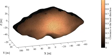
In the second strategy the laser is pointed on a fixed direction towards the asteroid. Using a triangulation to approximate the asteroid surface, the intersection point is defined as the barycentre of the triangle of the asteroid mesh closest to the spacecraft position vector. In formula:

min s arccos

s·r_lsr kskkrlsrk

, (2)

rlsris the position of the laser with respect to the asteroid, and k · kis the Euclidean norm inR3. Figure 2 shows an example

where the laser beam direction points towards the minimum distance direction between the spacecraft center of mass and the asteroid surface, assuming the laser points towards the centre of the asteroid along they-axis.

−80 −60 −40 −20 0 20 40 60 80 100 −20

0 20 −40 −20 0 20 40

X [m] Y [m]

Z [m]

Thrust direction projection on desired direction

[image:2.612.325.555.365.473.2]

0 0.1 0.2 0.3 0.4 0.5 0.6 0.7 0.8 0.9

Figure 1. Example of surface points producing thrust directed along they-axis

−80 −60 −40 −20 0 20 40 60 80 100 −20

0 20 −40 −20 0 20 40

X [m] Y [m]

Z [m]

Closeness to the laser direction

0 0.1 0.2 0.3 0.4 0.5 0.6 0.7 0.8 0.9

Figure 2. Example of surface points producing thrust directed along the laser beam direction

Deflection Efficiency

[image:2.612.323.555.526.640.2]

(3)

magnitude is calculated at predefined time intervals, called checkpoints. Lettcheckbe the instant of time corresponding

to a generic checkpoint, defined on the nominal trajectory as the true anomaly of the asteroidθcheck. The variation of

the position of the asteroid after deviation, with respect to its unperturbed position, can be written using the proximal motion equations [6]:

δr(tcheck) =Acheck(θcheck)δα(tcheck), (3)

wherer= [δsr, δsθ, δsh]T is the displacement in the radial,

transversal, and out of-plane directions in the Hill’s reference frame centered at the unperturbed position of the asteroid at the checkpoint, δα = [δa, δe, δi, δΩ, δω, δM] is the variation of the Keplerian orbital elements of the asteroid at the checkpoint, andAcheck(θcheck)is the matrix

transforma-tion between the variatransforma-tion of the orbital parameters and the trajectory displacements at the corresponding θcheck. The

magnitude of the total deflectionδr = ||δr|| represents the deflection parameter, which will be studied in the uncertainty analysis. The assumption used to compute displacement is that the variation of the relative positionδris small compared to the unperturbed orbit radiusrcheck, that isδrrcheck.

In order to perform fast simulations we used averaged quan-tities to be used in Eq. (3), exploiting the fact that on several rotations the mean direction and the fraction of useful thrust will depend on the shape of the asteroid, angular velocity and relative position of the laser. In fact the mean thrust calculated over∆tdays of operations will be

F= 1

T

Z t0+∆t t0

F(ωt,pl,S, P)dt , (4)

where F(ωt,pl,S, P) descends from the strategies

imple-mented in Eqs. (1) and (2); ω is the angular velocity, pis the position of the laser,Srepresents the geometry influence, andPl is the power available at the laser (see Section 3 for

details). The mean direction of thrustdand thrust efficiency

klwill be

d= F

F , (5)

kl=

F F(ωt0,pl,r¯A, P)

, (6)

where F(ωt0,pl,r¯A, P) is the magnitude of the nominal

thrust for a circular object of mean radius ¯rA att0, and F

is the magnitude of the mean thrust. In this way during the propagation of Eq. (3), we can refer to the nominal available thrust, which varies with the distance from the sun and the contamination level during the duration of the mission.

Another important element whose effects could produce vari-ation of the laser efficiency during the mission is represented by the mean variation of the angular velocity

dω= 1

T

Z t0+T t0

I−1(rl(t)×F(t))dt , (7)

where I is the matrix of inertia of the asteroid and rl is

the application point of the laser (also of the force). For simplicity, we do not consider the variation of the inertia because it is not significant during our analysis, although it will be consider in future works.

3. LASER-MATTER

INTERACTION

MODEL

This section describes the laser-matter interaction responsible for the thrust imparted on the asteroid. We first show the derivation of the moment coupling coefficient. Then we explain how to predict the contamination resulting from the fraction of the vaporized ejecta impinging on the solar arrays. Eventually it is described the defocusing process, when the distance between the laser and asteroid surface does not coincide with the focal length of the focusing optics.

Mechanical Coupling

The aim of the laser model is to predict the change in momentum imparted to the asteroid depending on its physical and dynamical properties and the key parameters of the laser system, namely the output power and the focusing capabili-ties. The key metric of the ablative deflection method is given by the thrust coupling coefficient, which is defined as

Cm= F

P , (8)

and represents the ratio between the thrust magnitudeF and the optical powerPinvested in the process.

To account for the tumbling rate of the asteroid, the cou-pling coefficient is recovered after solving the 1D transient equation. An enthalpy formulation is selected in Eq. (9), allowing for a more convenient way to handle the different phase transitions:

∂(ρH)

∂t =− ∂q ∂z+

∂(ρuH)

∂z , (9)

whereρdenotes the density in the condensed material,H is the enthalpy,qis the heat flux,uis the recession speed,tis the time, and z is the deep direction. The recession speed

u depends on the liquid/gas interface temperature Ts only

[7] and can be computed using the Hertz-Knudsen-Langmuir formula. The heat flux qis expressed through the common Fourier law q = −k dT /dz. Equation (9) can be solved numerically by takingNcells along the depth directionzand applying the conservation of the enthalpy to each of them as follows:

d(ρH)i dt =−

qi+1/2−qi−1/2

∆z +u(T1)

(ρH)i+1−(ρH)i

∆z ,

(10) whereiis the index of the cell andT1is the surface

tempera-ture. The heat fluxes are then computed from the Fourier law using central differences:

qi+1/2=−k

Ti+1−Ti

∆z , (11)

qi−1/2=−k

Ti−Ti−1

∆z . (12)

For convenience, the enthalpy is defined from an arbitrary reference value of 0 at the melting temperature Tm. With

this choice of reference, the temperature and the enthalpy are linked through

Ti=     

   

Tm+ Hi

cs

ifHi≤0,

Tm if 0< Hi< Em,

Tm+

Hi−Em cl

ifHi≥Em,

(4)

wherecsandclare the heat capacities in the solid and liquid

phases, respectively. At each time-step, the temperature can be recovered from the enthalpy and is fed into Eq. (11) which allows computing the enthalpy at the next time-step. The boundary conditions are then introduced through

q1−1/2=AΦ−qrad(T1)−ρu(T1)Ev, (14) qN+1/2=−k

T∞−TN

∆z . (15)

The boundary conditions for q1−1/2 simply states that the

heat flux conducted through the gas/liquid interface equates the transmitted flux intensityAΦto which is subtracted the flux radiatedqrad(approximated from the Stefan-Boltzman

law of emission of a black body) and the heat required to vaporize the flow crossing the interfaceρuEv. Equation (10)

is integrated in Matlabc using ode23t, which is suitable for moderately stiff problems. During the time-integration, the pressurepeand velocityvein the gas on the edge of the

Knudsen layer are reconstructed from the surface temperature Tsusing the jump conditions developed by Knight [7], which

allows for computing the real time evolution of the momen-tum coupling coefficient

C_mtr= pe+ρev

2

e

Φ =

(γ+ 1)pe

Φ . (16)

The actual coupling coefficientCmis then simply obtained by

averaging its value over the time of exposition of the surface

Cm= 0.87

τ

Z τ

0

Cmtrdt , (17)

in which the 0.87 factor accounts for the losses due to the Gaussian energy distribution of the main transverse electro-magnetic mode (TEM00) in the laser beam [8]. Considering

the relative velocity of the ablated surface to the laser beam vrel and the diameterφof the laser beam, respectively, the

mean heating timeτcan be computed as

τ =π 4

φ vrel

. (18)

Thus, an increased velocity of the illuminated surface with respect to the laser beam will reduce the time available to heat a given point.

We consider in this paper a rocky S-type asteroid essentially made of forsterite for which the relevant properties can be reviewed in Table 1. In particular, the mean value of the vaporization enthalpy has been reconstructed from the ther-mochemical properties of the different reactants and products assuming a diatomic gas mixture of magnesium oxide, silicon oxide and dioxygen is formed from the vaporization of the forsterite molecule [1], [9]. While all these properties are used in the computations, the importance of the absorptivity, the thermal inertia, and the vaporization enthalpy can be highlighted. The vaporization enthalpyEv drives the

min-imum amount of energy required to vaporize one kilogram of asteroid material. The thermal inertia, which is equal to the square root of the product between the density ρ, heat capacity c, and thermal conductivity k, drives the pace at which the asteroid material reaches a thermal equilibrium when heated. A lower value means thus that the steady-state regime of Eq. (9) is reached quicker. The additional conduction losses during the transient regime are also lower in this case because the material needs to store less energy

[image:4.612.314.560.104.284.2]

before the standing evaporation wave of the regime state can develop. Eventually, the absorptivity A of the material drives how much of the laser energy in the incident beam is not reflected (lost) by the surface of the asteroid.

Table 1. Assumed Physical Properties of an S-Type Asteroid

Property Symbol Value Unit

Density ρ 3280 kg/m3

Thermal conductivity k 2 W m−1K−1 Heat capacity (liquid) cl 1464 J kg−1K−1

Heat capacity (solid) cs 1264 J kg−1K−1

Vaporization enthalpy Ev 14.163 MJ kg−1

Melting enthalpy Em 0.508 MJ kg−1

Reference temperature Tref 3000 K

Saturation pressure (Tref) pref 4448.9 Pa

Melting point Tm 2171 K

Gas constant R∗ _206.7 _{J kg}−1_K−1

Heat ratio (gas) γ 1.26

-Emissivity 0.9

-Absorptivity A 0.8

-Rest temperature T∞ 298 K

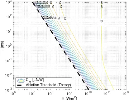
The results obtained by this model for forsterite are rep-resented in Figure 3. The black dashed curve represents

5

10

15

20

25

30

35

40

45

50

55

60

Φ [W/m2]

106 107 108 109 1010 1011 1012

τ

[ms]

10-3

10-2

10-1

100

101

102

103

C_m [µN/W]

Ablation Threshold (Theory)

Figure 3. Thrust coupling coefficient as a function of the mean heating timeτand the optical flux

the ablation onset for the forsterite material, which in log-arithmic scales appears as a line such thatΦ√τ = 0.106· 108_{W m}−2_s1/2_.

Contamination

The contamination model was adapted from the work of Kahle et al. [1]. From the surface temperature, the density

ρe and the velocity ve are computed on the edge of the

Knudsen layer where, for an expansion in vacuum, the flow reaches the local speed of sound. The model assumes two different flow regimes in the near field and in the far field. According to [1], the density at an arbitrary distance r from the reservoir and angle θ measured from the local surface normal is approximately given in the continuum flow regime as

ρ(r, β) =ρeAp φ2

(2r+φ)2

cos

_πβ

2βmax γ−21

[image:4.612.329.536.340.500.2]

(5)

The jet constant Ap and the limiting expansion angleβmax

are assumed to be equal to 0.345 and 130.45 degrees, respec-tively. Considering an isentropic expansion of the plume, the stagnation pressurep0and densityρ0can be computed using

the relations

ρe ρ0

=

1 + γ−1 2

γ−−11

, (20)

pe p0

=

1 + γ−1 2

γ−−γ1

. (21)

Similarly, the Mach number M, pressure p, and the velocity in the continuum regime are given by

M2= 2

γ−1

_ρ

ρ0

1−γ

−1

, (22)

p p0

=

1 + γ−1 2 M

2

γ−−γ1

, (23)

v= s

γM2_p

ρ . (24)

The transition from the continuum regime to the free molecu-lar regime happens when the distances between the molecules becomes too large for them to interact. In his simplified model, Kahle et al. [1] proposes using a sudden transition when the mean free path of the molecules lmfpbecomes larger than the beam diameter:

lmfp= kT

p√24πr2

mole

> φ , (25)

with the molecular radius rmoleestimated around 2·10−10m. Once the flow is in the free molecular regime, the assumption is that the velocity becomes constant while the density still decreases with respect to the inverse of the quadratic distance to the spot. The contamination model then assumes that only a fractionxsof the particle impinging on the solar array will

stick to it so that the growth of the contamination layer over time can be predicted as

dmA

dt =xs·G(ψ)·v(r, β)·ρ(r, β), (26)

whereψrepresents the angle between the normal to the solar panels and the impingement direction of the plume. The view function G is defined as following:

G= (

cos(ψ) if −π 2 < ψ <

π

2

0 otherwise . (27)

Assuming the arrays are pointed towards the sun and laser remaining in the same orbital plane during the operations, we have

cos(ψ−β) =− he

a(1−e2₎_V sin(θ), (28)

where h is the angular momentum, e the eccentricity of the orbit, V the velocity of the spacecraft, andθthe true anomaly. Finally, a degradation factor χ can be computed using the Beer-Lambert-Bougier law:

χ(t) = exp (−αmA(t)), (29)

whereαis the mass attenuation coefficient, which is about 104 _cm2_/g _{for forsterite [1].} _{From experimental}

investi-gations, we found that this contamination model predicts correctly the contamination level with a sticking coefficient

xs of 0.5 [10]. Over the course of the deflection action, a

contamination layer will grow on the solar arrays with the degradation factor decreasing slowly from an initial value of 1. This will reduce over time the available input power to the laser system.

Defocusing process

The variation of the deflection time with the defocus of the beam is however a function of the rotation rate. A variation of the distance will produce a bigger cross section Aspot

of radiuswon the surface of the asteroid consistently with the Rayleigh length lRayleigh, as shown in the following

equation:

w(l) =w0

s

1 + |l−lf ocusing|

lRayleigh

, (30)

Aspot=πw2=πw20

1 +|l−lf ocusing|

lRayleigh

, (31)

where l is the distance from the spot, and lf ocusing is the

focusing length. The light intensity at the spot decreases as the distance of the laser source from the surface departs from the focusing distance. If the incident laser beam is not perpendicular to the surface, the spot deforms from a circle to an ellipse and its area increases. Therefore, instead of calculating the exact traveling time, the light intensity is simply reduced by modifying Eq. (31) as follows:

Aspot=πw20

1 +|l−lf ocusing|

lRayleigh

1

cosθ¯, (32)

whereθ¯is is the angle between the incident laser beam and local normal. The area given by Eq. (32) is then used to calculate the current power flux. As one can see as the cross section increases with this angle, the power density decreases and progressively reduces to zero for nearly tangential con-figurations. In the following analysis, both perfect focus and defocus were considered. Nonetheless, the effect from the laser direction was held because it is not physically possible to eliminate this undesired effect.

4. UNCERTAINTY

MODEL

Unlike monoatomic substances such as aluminium, an aster-oid can be composed of a variety of substances which are loosely attached together. The exact composition as well as the degree of porosity affects, in turn, a series of key parameters driving the efficiency of the laser-matter inter-action process. Since it is not possible to know the exact composition and characteristics of the asteroid, we assume that these key parameters are only known with some degree of uncertainty. In the following analysis, we follow the approach presented in [11] to perform preliminary uncertainty analysis on a relevant subset of the parameters presented in Table 1. Both aleatory and epistemic uncertainty have been considered to assess the success of a deflection outcome.

Aleatory and Epistemic Uncertainty

(6)

reduced; they are generically well quantified with a known distribution. Epistemic uncertainties represent the potential deficiency that is due to a lack of knowledge; they include model uncertainties and uncertainty on the probability of an event, therefore, they cannot be fully captured with a single distribution or by assuming a known correlation among the variables.

When all the uncertainties are aleatory, the probability of an eventAis given by

P(A) =E[IA] = Z

A

p(u)du, (33)

whereIAis the indicator of the setAdefined as

IA(u) =

1 ifu∈A

0 otherwise , (34)

andp(u)is the product of the marginal probability densities associated with the uncertain quantities.

In our problem, we are interested in the probability of success of a deflection using the methods explained in Sections 2 and 3, thenAis the subset in the initial uncertainty spaceU ⊆RN

such that the deflection parameterδris greater than a fixed thresholdd∗, in formula

Ad∗={u∈U|δr(u)≥d∗}. (35)

The valued∗belongs to the interval[d, d], withd, dthe upper and lower limits of the deflection parameter given by

d= min

u∈Uδr(u), d= maxu∈U δr(u), (36)

which represent the worst- and the best-case scenario, respec-tively, under uncertainty.

An approximation of the integral in Eq. (33) can be obtained usingM sample pointsui, i= 1, . . . , Min the initial domain U ⊆_RN_{. Then the integral becomes}

Z

Ad∗

p(u)du≈ 1 M

M X

i=1

IAd∗(ui)p(ui), (37)

whereIAd∗is the indicator function of the setAd∗in Eq. (35).

A possible choice for the sample points can be the Carte-sian grid, thus the quadrature scheme becomes deterministic. Such a grid, however, would require to decide in advance how fine the grid should be, and all the grid points need to be used, which is unfordable in high dimension. An alternative approach is to use quasi-random number sequences, also called low-discrepancy sequences, which have the flexibility of pseudo-random number generators and the advantages of a regular grid [12].

Epistemic uncertainties are included using a parametric dis-tribution approach. The actual probability distribution is unknown but belongs to a set whose upper and lower proba-bilities are known. In this work, we used the beta distribution functions with unknown real positive parametersαandβ:

Bα,β(x) =

Γ(α+β) Γ(α)Γ(β)x

α−1₍₁₋_x₎β−1_, ₍₃₈₎

forx∈[0,1], whereΓ(z)is the Gamma function.

The upper and lower probability distributions are the solu-tions of the two optimization problems

min α,β

Z

Ad∗

p(u)du, max α,β

Z

Ad∗

p(u)du, (39)

where α and β are vectors of the same dimension of the epistemic parameters and each marginal density masspj, j= 1, . . . , N is now a beta distribution function with parameters

αj, βjforj= 1, . . . , N.

The computation of the the exact integral in Eq. (39) can be approximated using low-discrepancy sequences, as in the aleatory case,

min α,β

X

i Y

j

pj(uj,i),

max α,β

X

i Y

j

pj(uj,i), (40)

wherei ∈ {i|ui ∈ Ad∗} andj is a variable index. Once

the value of the two extreme beta distributions are found for

d∗, the exact upper and lower expectations can be refined by solving the multidimensional quadrature problem with a higher number of sample points.

The computation of the expectations requires to evaluate the dynamical model in thousands of sample points. To speed up the evaluation while maintaining an acceptable level of accuracy, we use a nonlinear representation of the uncertainty region of the deflection parameter given by a truncated series in Tchebycheff polynomials defined on a Smolyak sparse grid [13].

Uncertainty propagation

Uncertainty propagation methods can be divided into two groups: intrusive and non-intrusive. Intrusive approaches require a modification of the original problem by introducing a new algebra or by directly embedding high-order polyno-mial expansions of the uncertainty quantities in the governing equations. Non-intrusive approaches are instead based on a polynomial representation built on samples of the system response to the uncertainty quantities. The latter have the main advantage of working with generic models, also in the form of black boxes, and with little requirements on the coding of the models or on their regularity.

Following the work of Judd et al. [14], a non-intrusive method with truncated Tchebycheff series on sparse grids with Tchebycheff nodes has been used. Sparse grids al-lows for the representation of points on a hyperrectangle and further reducing the computation cost of the polynomial approximation problem. For example, a complete polynomial basis of maximum degree4in10unknown variables would require1 001 sample points, while the corresponding sparse grid contains only221points.

Letnbe the number of uncertainty variables and µ ∈ _N+

be the level of approximation of the sparse grid. Then the complete polynomial basis is given by

B={Tα1,Tα2 . . . ,Tαs}, s∈N

+_, ₍₄₁₎

whereαi= (αi1, . . . , αin)denotes the multi-index array

cor-responding to thei-th multidimensional Tchebycheff polyno-mial

Tαi = n Y

j=1

(7)

chosen in the space of all polynomials of degree at most2µ_in nvariables such that it satisfies the Smolyak rule at levelµ;

Tα_ij is the univariate Tchebycheff polynomial corresponding

to the variable of indexj. For example, forn= 2andµ= 1 the Smolyak rule gives

αi∈ {(0,0),(1,0),(0,1),(2,0),(0,2)}, (43)

and the corresponding Tchebycheff polynomial basis is

T(0,0)= 1, T(1,0)=x ,T(1,0)=y ,

T(2,0)= 2x2−1, T(0,2)= 2y2−1. (44)

For a fixed the level of approximationµ, the maximum degree of expansion is2µ_.

With a similar construction, Tchebycheff points on a Smolyak sparse grid have been computed. In [14] a new method to reduce the computation cost of the sparse grid and avoid repetition has been presented. The number of polynomial basis functions, which is equal to the number of points in the sparse grid, are shown in Table 2 for different values of the levelµand number of variablesn.

Table 2. Number of Elements in a Sparse Grid

µ/n 1 2 3 4 5 6

0 1 1 1 1 1 1

1 3 5 7 9 11 13

2 5 13 25 41 61 85

3 9 29 69 137 241 389

4 17 65 177 401 801 1457

5 33 145 441 1105 2433 4865

6 65 321 1073 2929 6993 15121

Let us denote with u0 the initial uncertainty variables that

belong to an hyperrectangle andf(u0)the response function.

Then the latter can be approximated with the truncated series

ˆ

f(u0) =

X

α∈Hn,µ

cαTα(u0), (45)

where eachcα represents the unknown coefficient with

re-spect to the elementTα, andHn,µas defined by the Smolyak

rule. The unknown coefficients can be computed by inverting the linear system

HC =Y , (46)

with

H = 



Tα1(u1) . . . Tαs(u1)

..

. . .. ...

Tα1(us) . . . Tαs(us) 

, C = 



cα1

.. .

cαs 

, Y = 



Y1

.. .

Ys 

,

where u1, . . . ,us are the Tchebycheff nodes in the sparse

grid and the components of Y are the evaluation of the response function in these points. The system in Eq. (46) cannot be inverted if the matrix H does not have full rank. In most of the cases, this is guaranteed by choosing the Tchebycheff nodes, which are equal in number to the number of unknown coefficients.

5. NUMERICAL

EXPERIMENTS

This section contains the outcome of a deflection using laser ablation for a hypothetical impactor on four cases:

1. Optimal thrust with focus. 2. Fixed thrust with focus. 3. Optimal thrust with defocus. 4. Fixed thrust with defocus.

The difference between the first two cases and the the last ones stands in the laser system capability of being able to adjust its focus or not.

A suitable reference trajectory is the one of 2013XK22, which is one of the few NEOs in the range of 50 m in mean radius with Keplerian orbital elements2(a, e, i,Ω, ω) = (1.045 AU, 0.2034, 6.95◦, 182.636◦, 265.7034◦). All the simulations start at the asteroid perigee. We used the shape of the asteroid (433) Eros scaled down to the correspondent mean size with 1708 facets of the discrete surface mesh. For the laser we considered an optics able to produce a diffraction limited beam of 3 mm at the focal length (300 m). With these parameters, the Rayleigh length is approximately equal to6m.

We restricted our uncertainty analysis to the parameters that define the size and characteristic of the asteroid (mean ra-dius ¯rA, density ρ, and angular velocity ω) and three key

parameters that define the laser model (vaporization enthalpy

Ev, thermal conductivityk, and absorptivityA). The initial

uncertainty space is the same for all the cases. Table 3 reports the upper and lower limit for each variables. Due to the lack of precise information about the asteroid size drawn from the imprecise optical observation for small objects, we assume a maximum uncertainty of20m with respect to the nominal size of the asteroid. For what concern the density, we consider that the asteroid will be a S-type one. The variability here can be due to the fact that the asteroid could be rubble-pile porous and its density can be as low as 2000 kg/m3_.

The angular velocity is then calculated as the self-attracting asteroid, which is based on the density boundaries [15].

[image:7.612.65.283.308.404.2]

During the vaporization process, the properties of the mate-rial can change substantially with the temperature. This is the reason why the limits for the vaporization enthalpy are placed at±20%with respect to the nominal value reported in Table 1. The same arguments apply to the case of the thermal conductivity, which can undergo huge variations between the different materials or simply because of the porous nature of the material. The value of5 can be considered as a worst-case scenario while a value of0.5would be consistent with the reported thermal inertia of asteroids. Hence, an order of magnitude of possible variation between these two values was considered. For the absorbivity the variation was assumed to be about ±20% with respect to the nominal case, which is consistent with the reported albedo values of S-type asteroids.

Table 3. Bounds for the Uncertainty Parameters

Variable Lower Limit Upper Limit

¯

rA[m] 30 70

ρ[kg/m3_] ₂₀₀₀ ₃₃₀₀

ω[rev/day] 5.1411 26.4156

Ev[MJ kg−1] 11 330 400 16 995 600

k[W m−1_K−1_] _0.5 ₅

A 0.7 0.9

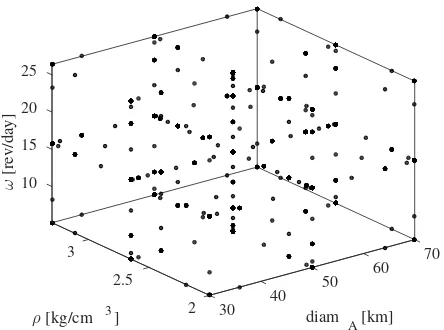
The bounds of Table 3 define a 6-dimensional hyperrectangle that has been sampled using the Smolyak sparse grid for dif-ferent levels of approximationµ. The corresponding number

[image:7.612.52.299.527.601.2]

(8)

of sample points is shown in the last column of Table 2. Figure 4 shows the points in ther¯A-ρ-ωspace forµ= 3.

70

diam A [km]

60 50 40 30 2 2.5

ρ [kg/cm 3]

3 25

20

15

10

ω

[image:8.612.320.550.49.229.2]

[rev/day]

Figure 4. Sparse grid points forµ=3

The other characteristics for simulating the laser ablation processes are reported in Table 1. The quantity of interest is the deflection parameter given by Eq. (3). Different deflection periods T and available powers P have been tested. We considered the discretisationT = 2,4,7,9,12,16,20years andP = 1,2,4,7,9,10,12,14,16,18,20kW. Note that the power is the input power at the laser, where a conversion efficiency of 55% was applied.

Nominal Deflection

The deflection parameter has been computed for each point in the sparse grid and each combination of period and power. Figures 5, 6, 7, and 8 show the variation of the deflection parameter as a function of period and power only and keeping the uncertainty parameters fixed at their mean values. As expected from [4], the performances of the laser deflection decreases passing from an optimal thrust to a fixed thrust direction. After 20 years, the maximum deflection due to the fixed direction strategy reduces by 15% from about 16 Earth radii. The focus/defocus strategies show similar results with another overall 15% efficiency loss.

1

1 1

2 2

2

3 3

3

4

5

5 5

6

6 6

7 7

8 8

9 9

10 10

11

12 13

14 15

Deflection Time [years]

2 4 6 8 10 12 14 16 18 20

Power at t

0

[kW]

2 4 6 8 10 12 14 16 18 20

[image:8.612.63.285.97.262.2]

Achieved Deflection [Earth radius]

Figure 5. Achieved deflection with optimal thrust with focus (case 1)

1

1 1

2 2

2

3 3

3

4

4 4

5

5 5

6 6

7 7

8 8

9 9

10

11 12

13

2 4 6 8 10 12 14 16 18 20

Power at t

0

[kW]

2 4 6 8 10 12 14 16 18 20

Figure 6. Achieved deflection with fixed thrust with focus (case 2)

1

1 1

1

2

2 2

3

3 3

4 4

4

5

6 6

7 7

8 8

9 9

10 11

12 13

14

2 4 6 8 10 12 14 16 18 20

Power at t

0

[kW]

2 4 6 8 10 12 14 16 18 20

Figure 7. Achieved deflection with optimal thrust with defocus (case 3)

1 1

1

2

2 2

3

3 3

4 4

5 5

6 6

7 7

8

9 10

11

2 4 6 8 10 12 14 16 18 20

Power at t

0

[kW]

2 4 6 8 10 12 14 16 18 20

[image:8.612.321.551.528.706.2]

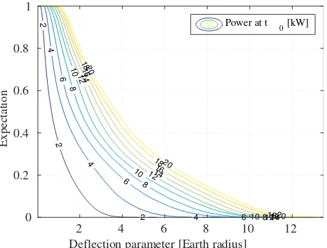
[image:8.612.60.292.530.706.2]

(9)

Uncertainty Analysis

We are interested in studying the expected probability of the success of the deflection method proposed in this paper, that is, the quantityE[IAd∗] given by Eq. (33) with the set Ad∗ defined in Eq. (35). In our simulations the deflection

parameter is δr = ||δr(tcheck)||, i.e., the magnitude of

the deviation with respect to the nominal trajectory at the checkpointtcheck as given in Eq. (3). The fixed threshold d∗is defined as multiple of the Earth radius.

The surrogate model was built using the Tchebycheff poly-nomial approximation explained in Section 4. The reliability of this approximation is shown in Table 4. The accuracy is represented with the root mean square error in km

σRMSE=

v u u t

1

M M X

i=1

( ˆδr(Xi)−δr(Xi))2, (47)

whereXi, i= 1, . . . , M are the evaluation points (different

from the sample points) andδr(Xi),δrˆ(Xi)are the exact and

[image:9.612.322.556.88.263.2]

predicted values, respectively, at each points. In the following analysis we will use a polynomial approximation of levelµ= 3since it gives a maximum error of a half Earth radius for the four cases.

Table 4. Tchebycheff Polynomial Approximation Accuracy for the Four Cases forT= 7Years and

P = 20kW

µ Case 1 Case 2 Case 3 Case 4

1 8.48e3 1.04e4 4.91e3 9.16e3 2 1.45e3 3.32e3 1.76e3 3.98e3 3 8.07e2 5.22e2 6.72e2 3.328e3

Aleatory Expectation—We assume that the uncertainty as-sociated with all uncertainty variables is aleatory and each marginal probability mass is a beta distribution function with parametersα = 1andβ = 1. The upper and lower limits in Eq. (36) of the deflection parameter are computed using a numerical solver called Inflationary Differential Evolution Algorithm (IDEA) [16]. The expectationE[δr≥d∗]is

com-puted using the approximation formula in Eq. (37) with sam-ple points taken in the Halton low-discrepancy sequence [17]. Figures 9, 10, 11, and 12 show the expectations for different

2

2 4

4

6

8

10

12

14

14 16

16

16 18

18

18 20

20

Deflection parameter [Earth radius]

2 4 6 8 10 12

Expectation

0 0.2 0.4 0.6 0.8 1

Power at t ₀ [kW]

Figure 9. Aleatory expectation for case 1 forT = 7years

values of the available power and fixed deflection time at

T= 7years.

2

4

6

6 8

8

8 10

10

12

14

16

18

18 20

20

5 10 15 20

Expectation

0 0.2 0.4 0.6 0.8 1

Power at t ₀ [kW]

Figure 10. Aleatory expectation for case 2 for T = 7years

2

2 4

4

6

8

10

12

12 14

14

16

16 18

18

18 20

20

2 4 6 8

Expectation

0 0.2 0.4 0.6 0.8 1

Power at t

[image:9.612.318.556.88.709.2]

0 [kW]

Figure 11. Aleatory expectation for case 3 for T = 7years

2

4

6

8

8 10

10

10 12

12

12 14

14

14 14

16

16 18

18

20

5 10 15 20 25

Expectation

0 0.2 0.4 0.6 0.8

Power at t

[image:9.612.73.279.322.408.2] [image:9.612.321.554.436.700.2]

0 [kW]

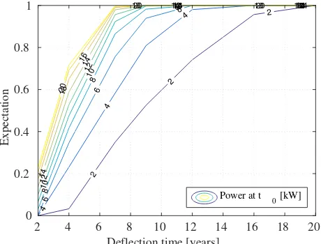
[image:9.612.62.295.538.715.2]

(10)

The cases with defocus reduce the maximum deflection by about 3 Earth radii. We see that the fixed deflection case presents more samples with higher deflection levels. At first sight the results of the expectation could appear surprising, contradicting the trend shown before with the mean values of the grid. In fact the fixed direction cases (with or without perfect focusing) present major deflections with respect to the optimal ones. Looking into details this behaviour is shown only by high power levels (i.e., P ≥ 10kW). The principal reason for this must be searched in Eq. (7), which produces perturbing torques in the case of the optimal thrust with subsequent rotational acceleration and efficiency drop. This effect is appreciable in only a small number of samples, when the inertia is small. Nonetheless, if we fixedd∗ _{= 1}

Earth radius, and we compute the expectationE[δr≥d∗]as a

function of time and power, we see that the overall behaviour works as expected from the previous mean values analysis. In fact the results of Figures 13, 14, 15, and 16 show that the time to deflect by one Earth radius is statistically inferior in the case of optimal deflection, with the perfect focus case clearly outperforming the defocusing one.

2 2 2 4 4 4 4 6 6 6 6 8 8 8 8 10 10 10 10 12 12 12 12 14 14 14 14 16 16 16 18 18 18 20 20 20

Deflection time [years]

2 4 6 8 10 12 14 16 18 20

Expectation 0 0.2 0.4 0.6 0.8 1

[image:10.612.320.551.48.226.2]

Power at t 0 [kW]

Figure 13. Expectation to deflection of 1 Earth radius for case 1

2 2 2 4 4 4 6 6 6 6 8 8 8 8 10 10 10 10 12 12 12 12 14 14 14 14 16 16 16 18 18 18 20 20 20

2 4 6 8 10 12 14 16 18 20

Expectation 0 0.2 0.4 0.6 0.8 1

Power at t ₀ [kW]

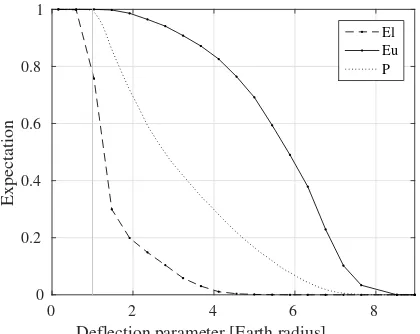
Upper and Lower Expectations—We now drop the assump-tion of perfectly known a priori probability distribuassump-tions and assume that the uncertainty associated with all uncertainty

2 2 2 4 4 4 6 6 6 8 8 8 8 10 10 10 10 12 12 12 12 14 14 14 14 16 16 16 16 18 18 18 18 20 20 20 20

2 4 6 8 10 12 14 16 18 20

Expectation 0 0.2 0.4 0.6 0.8 1

[image:10.612.322.551.272.452.2]

Power at t ₀ [kW]

2 2 2 4 4 4 6 6 6 8 8 8 10 10 10 12 12 12 14 14 14 16 16 16 18 18 18 20 20 20

2 4 6 8 10 12 14 16 18 20

Expectation 0 0.2 0.4 0.6 0.8 1

Power at t ₀ [kW]

variables are epistemic. The marginal probabilities are as-sumed to belong to sets of beta distributions with parameters

αand β such that 1 ≤ α, β ≤ 3. These parameters are then numerically optimised by solving Eq. (40) with IDEA for different values of the threshold deflection parameterd∗

to obtain the upper expectation Eu and lower expectation El. The approximated integrals in Eq. (40) are computed

[image:10.612.61.291.274.449.2] [image:10.612.63.291.457.668.2]

(11)

0 2 4 6 8 10 12

Expectation

0 0.2 0.4 0.6 0.8 1

[image:11.612.324.534.59.226.2]

El Eu P

Figure 17. Upper and lower expectation for case 1

0 5 10 15 20

Expectation

0 0.2 0.4 0.6 0.8 1

[image:11.612.60.269.59.227.2]

El Eu P

6. CONCLUSION

We presented and analysed two different control strategies combined with two laser pointing optics settings in terms of achieved deflection. The shape of asteroid (433) Eros scaled down to the considered size was used to simulate a 100 m-diameter real object. The interaction between the laser and the asteroid was modelled using high-fidelity model.

The composition and characteristics of the asteroid, and some key parameters of the laser matter model were assumed to be known with some degree of uncertainty. Both aleatory and epistemic uncertainties were taking into into account. Aleatory uncertainties were modeled with known distribu-tions. Epistemic uncertainties were treated using the para-metric distribution in which the marginal distributions were assumed to belong to a family of known distributions with unknown parameters.

We first simulated the behaviour of the different deflection systems using averaged quantities. Then, a surrogate model was built using Tchebycheff polynomial expansion, which gave a nonlinear map between the initial uncertainty space and the deflection parameter. Thus, the actual dynamics and laser model was replaced by a polynomial expansion in order to reduce the complexity of the uncertainty analysis.

0 2 4 6 8

Expectation

0 0.2 0.4 0.6 0.8 1

[image:11.612.64.273.272.439.2]

El Eu P

0 5 10 15 20

Expectation

0 0.2 0.4 0.6 0.8 1

El Eu P

We saw that the uncertainties affecting the deflection play an important role. Although the optimal focusing system yields the best results in terms of overall deflection, the unfocused system is still able to yield the one Earth radius deflection for many cases. For high power densities, this can be achieved in just a few years. From an operational point of view keeping the laser pointing fixed with no mechanism to adjust the focusing system will be preferable. Before sending an actual demonstration mission to deflect a small asteroid the deflection system will be known and these analyses could be used to design the laser-carrying spacecraft. In fact, the results of this paper can be applied to identify critical parameters in terms of mission duration, available power, asteroid control logic, and laser optics capabilities to achieve a certain deflection with a desired probability of success.

Future works will carry out a full sensitivity analysis to iden-tify which parameters most affect the deflection outcomes. A possibility is to study the problem without assuming any shape for the distribution. For this purpose, one could use the belief and plausibility function [18], in which the actual distribution is unknown but belongs to a set whose upper and lower probability distributions are known.

[image:11.612.322.528.274.442.2]

(12)

a spacecraft carrying the laser on the overall efficiency. For this purpose, onboard estimation and control systems will be simulated and used for the sensitivity analysis.

ACKNOWLEDGMENTS

This work is partially funded by the European Commission’s Framework Programme 7, through the Stardust Marie Curie Initial Training Network, FP7-PEOPLE-2012-ITN, Grant Agreement 317185. The authors would like to thank the unknown reviewers of this paper.

REFERENCES

[1] R. Kahle, E. K¨uhrt, G. Hahn, and J. Knollenberg, “Physical limits of solar collectors in deflecting Earth-threatening asteroids,”Aerospace Science and Technol-ogy, vol. 10, pp. 253–263, 2006.

[2] M. Vasile and C. Maddock, “On the Deflection of Aster-oids with Mirrors,”Celestial Mechanics and Dynamical Astronomy, vol. 107, no. 1, pp. 265–284, May 2010.

[3] M. Vasile, A. Gibbings, I. Watson, and J.-M. Hopkins, “Improved laser ablation model for asteroid deflection,” Acta Astronautica, vol. 103, pp. 382–394, 2014.

[4] M. Vetrisano, J. L. Cano, N. Thiry, C. Tardioli, and M. Vasile, “Asteroid’s orbit and rotational control using laser ablation: Towards high fidelity modelling of a de-flection mission,”Proceedings of the 25th International Symposium on Space Flight Dynamics, 19–23 October 2015.

[5] M. Vetrisano, C. Colombo, and M. Vasile, “Asteroid rotation and orbit control via laser ablation,”Advances in Space Research, vol. 56, no. 8, pp. 1547–1804, 2015.

[6] M. Vasile and C. Colombo, “Optimal impact strategies for asteroid deflection,” Journal of Guidance, Control and Dynamics, vol. 32, no. 4, pp. 858–872, 2008.

[7] C. J. Knight, “Theoretical modeling of rapid surface vaporization with back pressure,”AIAA journal, vol. 17, no. 5, pp. 519–523, 1979.

[8] N. Thiry and M. Vasile, “Deflection of uncooperative targets using laser ablation,” inSPIE Optical Engineer-ing + Applications. International Society for Optics and Photonics, 2015.

[9] ——, “Recent advances in laser ablation modelling for asteroid deflection methods,” inSPIE Optical Engineer-ing + Applications. International Society for Optics and Photonics, 2014.

[10] A. Gibbings, M. Vasile, I. Watson, J.-M. Hopkins, and D. Burns, “Experimental analysis of laser ablated plumes for asteroid deflection and exploitation,” Acta Astronautica, vol. 90, no. 1, pp. 85–97, 2013, NEO Planetary Defense: From Threat to Action.

[11] C. Tardioli and M. Vasile, “Collision and re-entry anal-ysis under aleatory and epistemic uncertainty,” AAS Astrodynamics Specialists Conference, Vail, Colorado, USA, August 9–13, 2015, AAS 15-709.

[12] R. E. Caflisch, “Monte carlo and quasi-monte carlo methods,”Acta Numerica, vol. 7, pp. 1–49, 1 1998.

[13] S. Smolyak, “Quadrature and interpolation formulas for tensor products of certain classes of functions,” Dofl. Akad. Nauk, vol. 158, pp. 1042–1045, 1963.

[14] K. L. Judd, L. Maliar, S. Maliar, and R. Valero, “Smolyak method for solving dynamic economic mod-els: Lagrange interpolation, anisotropic grid and adap-tive domain,”Journal of Economic Dynamics and Con-trol, vol. 44, no. 1-2, pp. 92–123, 2014.

[15] P. Pravec, A. W. Harris, and B. D. Warner, “Nea rota-tions and binaries,”Near Earth Objects, our Celestial Neighbors: Opportunity and Risk, Proceedings IAU Symposium. Edited by G.B. Valsecchi and D. Vokrouh-lick, and A. Milani. Cambridge: Cambridge University Press, no. 236, pp. 167–176, 2007.

[16] M. Vasile, E. Minisci, and M. Locatelli, “An Inflation-ary Differential Evolution Algorithm for space trajec-tory optimization,”IEEE Transactions on Evolutionary Computation, 2001.

[17] J. Halton, “Algorithm 247: Radical-inverse quasi-random point sequence,” ACM, vol. 7, pp. 701–702, December 1964.

[18] G. Shafer, “A mathematical theory of evidence,” Prince-ton University Press, 1976.

BIOGRAPHY

[

Massimo Vetrisanoreceived his M.Sc. degree in aerospace engineering from the Politecnico of Milan in Italy. He is finalizing his PhD under the guidance of Prof. M. Vasile at the University of Strathclyde, Glasgow, UK. Massimo took part in the European Student Moon Orbiter (ESMO) as flight dynamics spe-cialist and in the study for end-of-life and disposal concepts and asteroid de-flection missions. In 2013 he won the Space Generation OHB Move an Asteroid Competition in Beijing. His research interests include optimal estimation and control, uncertainty quantification, space robotics, and autonomous navigation. He is current an experienced researcher within the Stardust FP7 Marie Curie Initial Training Network at Deimos Space S.L.U. in Madrid, Spain.

(13)

Chiara Tardiolireceived her M.Sc. de-gree in mathematics from the Univer-sity of Pisa in Italy with a thesis on the propagation of orbit-crossing aster-oids. Her current PhD research involves studying new methods for active re-moval/deflection of noncooperative tar-gets under uncertainty, which is carried out within the frame of the Stardust FP7 Marie Curie Initial Training Network at the University of Strathclyde, United Kingdom.

Massimiliano Vasileis director of the Advanced Space Concepts Laboratory, and professor of Space Systems Engi-neering in the Mechanical & Aerospace Engineering Department at the Univer-sity of Strathclyde. Previous to this, he was a senior lecturer in the Department of Aerospace Engineering and head of research for the Space Advanced Re-search Team at the University of Glas-gow. His main research interests are space mission analysis and design, computational optimization, optimization under uncertainty, multidisciplinary design, asteroids, space flight mechanics, and autonomous robotic systems. He is a member of the IAF Space Power and Astrodynamics Committees.