Return and abort trajectory optimisation for reusable launch vehicles

Launch abort trajectory optimisation for reusable

launch vehicles

Federico Toso

and Christie Alisa Maddock

University of Strathclyde, Glasgow, G1 1XJ, United Kingdom

Among the future space access vehicles, the lifting body spaceplane is the most promising approach to prevent damage to both the launcher and the payload in case of loss of thrust. The glide performances of the vehicle allow the recovery in both nominal and abort cases. The approach presented is used in the investigation of the unpowered descent paths of a sample vehicle through trajectory optimisation. The vehicle’s downrange and crossrange limits are obtained for aborts in multiple flight conditions.

I.

Introduction

The main approach to deliver payloads into space has historically been the expendable vertically launched rocket. Recent advancements towards the partial or full re-usability of the first stages holds the potential to significantly lower the cost of access to space and open a broader market. One reusable launcher that could emerge in this market is the spaceplane, a lifting body vehicle can reduce the aerodynamic losses of the ascent and take advantage of effective air-breathing engines that do not require on-board storage of the oxidizer. Those hybrid or combined cycle engines are still at low to mid-levels of development, while chemical rocket engines are reaching their theoretical peak efficiency.

The use of recoverable first stages for space launchers requires the analysis of flight paths that the vehicle can follow to be recovered for refurbishment and future reuse. Due to the limited available locations that allow a safe horizontal landing in an airfield or spaceport, as well as the safety and regulatory requirements, planning for recovery and abort scenarios is a critical task that has to be included from a very early stage in the vehicle design process.

The vehicle considered in this study is a lifting body vehicle powered by a combined cycle engine. The performances of the vehicle are studied with a software1–3 _{for trajectory and multidisciplinary design}

optimisation (MDO) that is extremely modular and can change the mathematical models to cater for different needs of model accuracy or computational runtime depending on the requirements.

An initial study is performed to determine the best ascent profile under nominal conditions by optimising the trajectory of the vehicles to deliver the maximum payload to a target orbit. Abort scenarios are simulated at different points along the ascent trajectory by removing the propulsion (turning off the engine but keeping the fuel onboard) and optimising the glide descent path. The re-entry flight is optimised to find the maximum range that the vehicle can reach in both downrange and crossrange distance.

II.

System models

This section describes the mathematical models used to simulate the vehicle performance over the mission. Specifically, models are presented for 3DOF flight dynamics, open loop control of the thrust and vehicle attitude, propulsion system, vehicle aerodynamics, environment models for the Earth’s geometry, atmosphere and gravity.

A. Flight dynamics and control

The vehicles are modelled as a point mass in an Earth Centered Earth Fixed reference frame with 3 degrees of freedom for all phases of the mission. The state vectorx= [h, λ, θ, v, γ, χ] contains the 6 variables for position and velocity, explicitly defined as altitude h, velocityv relative to the reference frame, flight path angleγmeasured from the local horizon, heading angleχdefined clockwise from the local North, andλand

θ as latitude and longitude coordinates on the Earth. The derivatives of the state variables are calculated with,

˙

h= ˙r=vsinγ (1a)

˙

λ=vcosγsinχ

r (1b)

˙

θ=vcosγcosχ

rcosλ (1c)

˙

v=FTcosα−D

m −grsinγ+gφcosγcosχ+ω

2

ercosλ(sinγcosλ−cosγsinχsinλ) (1d)

˙

γ=FTsinαcosµ+L

mv −

gr

v cosγ−

gφ

v sinγcosχ+ v

rcosγ+ 2ωecosχcosλ (1e)

+ω_e2r v

cosλ(sinχsinγsinλ+ cosγcosλ)

˙

χ= Lsinµ

mvcosγ −gφsinχ− v

r

cosγcosχtanλ+ 2ω_e(sinχcosλtanγ−sinλ) (1f)

−ω_e2

r vcosγ

cosλsinγcosχ

where D andL are the aerodynamic lift and drag forces,m(t) is the mass of the vehicle andω_e is Earth’s rotational speed. The gravity is decomposed in two components of the force, the tangentialgφand the radial

gr. The vehicle controls are the direction and magnitude of the thrust vectorFT through the modulation of

the throttle, the angle of attackαand bank angleµof the vehicle. The propulsion system is non-gimbled; the thrust vector produced is aligned with the longitudinal body axis of the vehicle.

The coordinates are converted into the Earth Centered Inertial frame to compute the Keplerian orbital parameters for the semimajor axisa, eccentricityeand inclinationi.

B. Environment

The WGS84 geodetic system is used to model the Earth geometric parameters including the radius length from the centre to the Earth surface r/E as a function of latitude. The rotation of the planet is ωe =

7.292115e−5 rad/s.

The gravitation model is based on spherical harmonics accounting for theJ2,J3andJ4terms. The radial and tangential components of the gravitational pull are computed from the local radius rE, the vehicle’s

height above surfacehand the latitudeλ.

The atmosphere is modelled using the static global International Standard Atmosphere. The model is expanded above the maximum altitude hmax = 84852 m by extending the exponential laws regulating

pressure and density assuming constant temperatureT(h > hmax) = 186.87 K.

C. Vehicle configuration

The vehicle is a horizontal take off and landing, reusable launch vehicle originally designed for a target mission of releasing 1000 kg of payload in ah= 200 km circular orbit from a high latitude spaceport. The gross and dry mass values are obtained from the multidisciplinary optimisation3_{of a vehicle performed using}

the lift and drag coefficients for a conceptual hypersonic test vehicle Lazarus,4 _{a conceptual study focused}

on the development of aerodynamic laws for the purpose of scaling surfaces. This results in a vehicle with an optimised gross take off mass mgtow = 90035 kg and a dry mass ofmdry = 22907 kg, equal to an inert

mass marginmdry/mgtow = 0.254.

engine with reduced inlet area, the aerodynamics were recalibrated based on experimental wind tunnel test results for the X-34.5 A design optimisation aimed at sizing the propulsion system is performed concurrently with the ascent trajectory analysis.

D. Aerodynamics

The database5 _{of aerodynamic characteristics resulted from the studies of the X-34 vehicle presents an}

extended set of coefficientsCL andCD values gathered from wind tunnel tests. The data points cover a set

of inputs in a range of Mach number 0.4≤M ≤6 and angle of attack−4deg≤α≤24deg, while the Lazarus model is valid only in the supersonic regime. The database is used to create two functions CL=f(α, M)

and CD=f(α, M) obtained through polynomial interpolation. The order of the polynomial is the lowest

that guarantees a coefficient of determination R ≥ 0.99, assuring accurate results and fast computation. The R value is guaranteed inside the domain of the experimental test results for the X-34, therefore the controls of the vehicle are bound within the limits of angle of attack and Mach of the dataset. Whenever the Mach is outside of the experimental points range, the value is treated as equal to the closest bound in the interpolating equation. The reference aerodynamic surface of the vehicle is calculated by choosing the same take-off aerodynamic load of the X-34 test vehicle of W/Sref = 2423 N/m2, resulting in an area

Sref = 364.64 m2.

The upper stage configuration is an expendable rocket with a cylindrical body, no lifting surfaces. The aerodynamic model uses a constant drag coefficientCD = 1, lift coefficientCL = 0 and a reference surface

areaSref = 1 m2.

E. Propulsion

The first stage propulsion system is a hydrogen fuelled motor capable of functioning as both an air breathing engine, using atmospheric oxygen, and rocket, using onboard LOX at the catalyst. The use of a high-speed air breathing engine is the crucial requirement to reach a suitable LEO/LEO-injection altitude at a high velocity without a second stage. This can be achieved by a number of differing hybrid propulsion systems, such as ejector-ramjet-scramjet rocket combinations to the more integrated Synergistic Air-Breathing Rocket Engine (SABRE) under development by Reaction Engines.6 _{The engine performance here is modelled based}

on the published performance specifications for the SABRE.

The rocket maximum vacuum a specific impulse isIsp= 450 s, modelled using the general rocket equation

accounting for the nozzle expansion losses due to changes in atmospheric pressure.

At lower altitudes, generally below 30 km, the engine can exploit the presence of oxygen in the atmosphere and it is modelled as a modified rocket engine with variable Isp and performance depending on the flight

conditions. The maximum equivalent specific impulse isIsp= 6500 s. Increasing altitude negatively affects

this value due to the decrease of air pressure and density. Quadratic laws were developed that reach the peak efficiency value at M = 3.5 and 100% throttle to model this phenomenon. The thrust is computed with the equationT =mpg0Isp.

The switching point between the two engine operational modes is unconstrained and is a result of the optimisation of the ascent.

The upper stage is modelled as a small hydrazine thruster, with Isp= 250 s, and the same formulation

used for the nozzle losses of the first stage rocket.

The propellant mass flows for both stages and all engine operating modes are optimisation variables in the trade off analysis of the ascent. The descent cases analyses are set up as unpowered glides by imposing a zero throttle along the whole trajectory.

III.

Optimisation

The solution found is used as a first guess if multiple cases with similar starting conditions are analysed, such as the descent ones in the following sections.

A. Optimal control problem formulation

The optimal control problem is formulated with a direct transcription, multiple shooting method. The trajectory is divided innP user defined phases with different system models, control bounds or coarser/finer

meshes. Every phase is divided into nE segments with nC discrete control nodes. The nodes define the

control grid that is analysed during the trajectory propagation to determine the attitude of the vehicle. In this analysis the Chebyshev nodes are used and the values between the nodes are computed with a Piecewise Cubic Hermite Interpolating Polynomial. Each of the multiple phases is set up with the specific set of mathematical models and, in this case, numerically integrated with a 4th order fixed timestep Runge Kutta method following the control law.

The optimisation vector is constructed element by element, each of those blocks containing the values of the controls in the nodes, the initial state variables and the duration of the trajectory segment. The states and controls are matched between elements to guarantee a continuous flight. The values at end of a segment resulted from a trajectory propagation have to be equal to the ones at the beginning of the next segment. Additional equality constraints are set on the final values of the flight to reach desired conditions such as a predetermined orbit and to assure a correct mass separation when staging. Inequality constraints include acceleration and dynamic pressure limits. Inequality is also used if the final state values have to be greater or less than a defined amount. The tolerance on all constraints is 10−4_.

The algorithm used is the single objective sequential quadratic programming. The cost functions used for this analysis are the maximum payload, maximum downrange and crossrange distances.

B. First guess generation

To identify a suitable first guess, a pool of starting guesses from the search space is generated with Latin Hypercube Sampling and run through the optimisation routine with relaxed constraints and 3 times longer timestep, reducing the tolerance on both the equality and inequality ones to 10−3_{. This approach increases}

the exploration capabilities of the algorithm. The converged solution with best cost function is used for the analysed data presented.

This approach to find a solution closer to the global minimum is computationally expensive and well suited for single case analysis. In the study presented for the abort scenarios multiple points have to be evaluated, therefore the time and resources required to complete the calculations with such approach are prohibitive. The converged solutions are passed as ’warm start’ initial guesses to a second optimisation routine set with the original tolerances and timestep length.

Choosing closely spaced abort points means that the starting conditions of consecutive cases have minor differences and the solution for the previous starting point can be used to provide the optimisation routine with a good starting guess that can quickly converge to a solution and repeat the iterative process, sampling the whole search space only once.

IV.

Test cases and results

A. Nominal ascent trajectory

The nominal ascent mission is the deployment ofmp = 1000 kg of payload in a 200 km circular orbit. The

chosen starting location for the ascent at (0◦N,0◦E) latitude and longitude. Placing the origin of the axis in this location does not require reference frame transformations to compute distances. The same approach can be applied to any other starting point on Earth.

The aerodynamic model introduced requires a new evaluation of the optimal value of maximum thrust to reach the imposed objective. Two engine scaling parameters are added to the optimisation vector, one per stage. The first stage can scale the thrust levels of the air breathing mode in the range [2.5,4.8] MN, while the rocket vacuum maximum thrust is in the range [3.2,6] MN. The second stage boundaries are [500,5000] N.

The starting conditions of the ascent areh0 = 1000 m, v0= 150 m/s, γ0 = 0 deg,θ0 = 90 deg, λ0 = 0

−4 deg≤α≤24 deg and the throttle 0≤τ≤1. The upper stage has an initial massm0= 1000 kg and the initial starting conditions are part of the optimisation variables. The controls for the upper stage increase the range of available angle of attack to −30 deg≤α≤30 deg. The starting values of angle of attack and roll are constrained to be the same of the first stage at the instant of release, while the throttle is not.

The choice of starting the ascent from the intersection of Greenwich meridian and the Equator and eastward flight simplifies the visualization of the results; the impact of latitude of launch site and inclination of the target orbit has been extensively documented and analysed in past studies.3 _{The cost function to}

maximise in the ascent optimisation is the final payload mass.

The first stage flight is divided in two phases of ne = 3 multiple shooting elements, each with nc = 5

control points. The second stage has the task of circularizing the orbit by raising the perigee if the first stage cannot. A reduced number of elementsne= 2 is used in this phase, while the number of control points per

element remains constant.

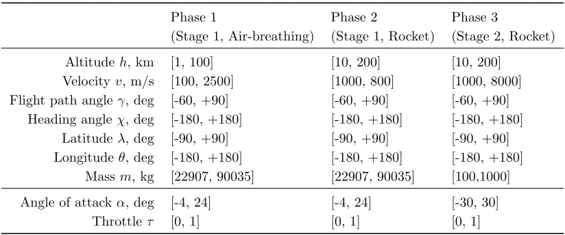
Table 1: Upper and lower bounds for ascent analysis

Phase 1 Phase 2 Phase 3

(Stage 1, Air-breathing) (Stage 1, Rocket) (Stage 2, Rocket)

Altitudeh, km [1, 100] [10, 200] [10, 200]

Velocityv, m/s [100, 2500] [1000, 800] [1000, 8000]

Flight path angleγ, deg [-60, +90] [-60, +90] [-60, +90]

Heading angleχ, deg [-180, +180] [-180, +180] [-180, +180]

Latitudeλ, deg [-90, +90] [-90, +90] [-90, +90]

Longitudeθ, deg [-180, +180] [-180, +180] [-180, +180] Massm, kg [22907, 90035] [22907, 90035] [100,1000]

Angle of attackα, deg [-4, 24] [-4, 24] [-30, 30]

Throttleτ [0, 1] [0, 1] [0, 1]

The optimisation results in a final massmp= 999.933 kg delivered to the target orbit. The mass lost by

the second stage is due to the very short circularization burn performed at the apogee. The optimised value of upper stage thrustT2= 500 N is on the lower bound. The reusable stage maximum thrust values for the

airbreathing and rocket mode are respectively TSL,max = 3.894 MN and Tvac,max = 4.984 MN. From the

throttle profile emerges the exploitation by the optimisation routine of the often used strategy of coasting to the apogee to raise the perigee.

B. Descent case analysis

The analysis of the abort trajectories uses the results generated from the ascent optimisation as starting point for the descent abort scenarios. The ascent throttle profile shows the separation between an initial powered phase in the air-breathing and rocket segments followed by a ballistic flight. During this phase, the vehicle will coasts till the apogee of the suborbital arc, where a final boost circularizes the orbit. This phenomena simplifies the problem allowing the study of the abort trajectories in the first 4 elements of the trajectory covering the main powered part of the ascent. After the engine cut off point the trajectory would closely follow a nominal ballistic suborbital arc followed by a final glide re-entry. With no thrust, no extra energy is introduced into the system. Studying any of the points after the end of the 4th_{element would yield}

similar results. A set of 50 data points is selected to guarantee a fine grid of starting points without being too computationally intensive. Those cover a set of altitudes 1 km< h0<108 km and velocities 271 m/s

< v0<6327 m/s. The points are equally spaced in time every 6 seconds along the ascent trajectory. The states variables corresponding to those selected points are used as starting conditions for each of the abort scenarios.

The descent phase is constrained to achieve a final state corresponding to a landing approach with an altitudehf = 1000 m, speedvf = 150 m/s and flight path angleγ <10◦. Given the assumption of equatorial

attack of the vehicle is therefore constrained between the limits of the aerodynamic model−4◦≤α≤24◦, while throttle and bank angle are fixed toτ = 0◦ andµ= 0◦.

The glide descent is composed of a single phase subdivided in ne= 3 multiple shooting segments, each

containingnc = 7 control points following a Chebyshev nodes distribution. The values of control between

the points are obtained with a piecewise cubic Hermite spline. The integration of the trajectory is performed with a 4th _{order RungeKutta method with fixed timestep. Constraints limit the peak accelerations and}

dynamic pressure respectively to |ax,z| ≤6g0 and max(Q)≤20 kPa. The distance from the starting abort

point, evaluated with the Haversine formula, is the maximised optimisation metric.

Table 2: Upper and lower bounds for the descent downrange and crossrange analyses

Altitude, km [1,200] Velocity, m/s [150, 8000] Flight path angle, deg [-60, +90]

Heading angle, deg [-180, +180] Latitude, deg [-90, +90] Longitude, deg [-180, +180]

Mass, kg [22907, 90035]

Angle of attackα, deg [-4, 24] Bank angle µ, deg [-80, 80]

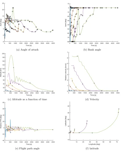
A further analysis is subsequently performed by adding the bank angle control −80 deg ≤µ≤80 deg starting from the same abort points to identify the crossrange capabilities of the vehicle. The bank angle rotates the lift vector around the velocity axis. The single phase of the downrange analysis is separated into two, the first one with 2 elements has the additional control of the bank angle. The last phase, made of a single element, remains with only the control of the angle of attack. This choice has been made because during the first trial runs a faulty behaviour emerged: The long duration of the reentry from higher starting energies and the coarse control mesh chosen made the vehicle enter spirals that reduced altitude without gain in crossrange capabilities. The chosen setup eliminates the problem and does not require an increased node number. In this case the optimisation metric is the maximum latitude. The total crossrange is obtained by calculating the arc length from the equator to the final latitude.

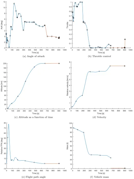
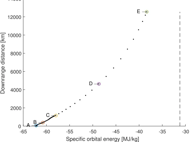
C. Maximum downrange results

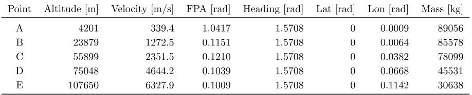
Out of the 50 points analysed, five points are chosen as representative of the group of solutions. The first four (A, B, C, E) are selected at the end of the respective ascent trajectory elements. A 5th _{one (D) is picked}

in the middle of the rocket flight segment. Table 3 lists the initial state vector for each point. The results for the downrange analysis are shown in Figs 2.

Table 3: Starting conditions of the selected result points highlighted in the descent graphs

Point Altitude [m] Velocity [m/s] FPA [rad] Heading [rad] Lat [rad] Lon [rad] Mass [kg]

A 4201 339.4 1.0417 1.5708 0 0.0009 89056

B 23879 1272.5 0.1151 1.5708 0 0.0064 85578

C 55899 2351.5 0.1210 1.5708 0 0.0382 78099

D 75048 4644.2 0.1039 1.5708 0 0.0668 45531

E 107650 6327.9 0.1009 1.5708 0 0.1142 30638

of the starting conditions. From the same values of altitude and velocity, the direction of the latter impacts the performances.

While the skip re-entry is a return strategy that has been used by many re-entry vehicles, it does present practical issues such as added stress on the structure, limitations on the lifetime of the vehicle (re-usuability), onboard control and stability, etc. The phugoids can be mitigated within the analysis through more strict acclerations/loading limits, h further constraints or post-processing of the controls though this would represent a suboptimal result considering only the maximum range possible. The focus of this study was to evaluate the maximum capability of the vehicle under emergency situations.

D. Maximum cross range results

Figures 4 show the time histories of controls and states in the descent case. It can be seen that the case with bank show the lack of significant aerodynamic forces in the high altitude suborbital arcs. The relation between crossrange and starting energy is shown in Figure 5.

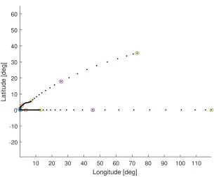
The combined locations of the coordinates of the final points are shown in Figure 6 on the latitude-longitude plane. The five sample points are highlighted to clearly show the distribution of solutions and therefore maximum range of glide flight of the vehicle.

V.

Conclusion

The downrange and crossrange distance performances in case of abort events during the ascent of a spaceplane have been studied. The results obtained can be applied to the study of the abort procedures from any launch site.

The first guess creation through multistart analysis on the first point and successive iterative generation approach has succeeded in providing results for all the abort points analysed. This technique reached convergence in all cases, eliminating the need of repeated explorative analysis, saving computational time. The energy-distance plots can be a useful tool to study trade-offs between vehicles, launch locations, abort procedures and risk assessment. The algorithm can also be used perform a MDO to satisfy regulatory or technological constraints.

References

1_{Pescetelli, F., Minisci, E., Maddock, C., Taylor, I., and Brown, R., “Ascent Trajectory Optimisation for a}

Single-Stage-to-Orbit Vehicle with Hybrid Propulsion,”AIAA/3AF International Space Planes and Hypersonic Systems and Technologies Conference, 2012.

2_{Toso, F., Maddock, C., and Minisci, E., “Optimisation of Ascent Trajectories for Lifting Body Space Access Vehicles,”} Space transportation solutions and innovations symposium, International Astronautical Congress, 2015.

3_{Toso, F. and Maddock, C., “Deployed payload analysis for a single stage to orbit spaceplanes,” Space transportation} solutions and innovations symposium, International Astronautical Congress, 2016.

4_{Young, D. A., Kokan, T., Clark, I., Tanner, C., and Wilhite, A., “Lazarus: A SSTO Hypersonic Vehicle Concept Utilizing}

RBCC and HEDM Propulsion Technologies,”International Space Planes and Hypersonic Systems and Technologies Conference, AIAA, 2006.

5_{Brauckmann, G. J., “X-34 vehicle aerodynamic characteristics,”Journal of spacecraft and rockets, Vol. 36, No. 2, 1999,}

pp. 229–239.

0 100 200 300 400 500 600 700 800 900 1000 Time [s] -4 -2 0 2 4 6 8 10 12 AoA [deg]

(a) Angle of attack

0 100 200 300 400 500 600 700 800 900 1000

Time [s] 0 0.1 0.2 0.3 0.4 0.5 0.6 0.7 0.8 0.9 1 Throttle

(b) Throttle control

0 100 200 300 400 500 600 700 800 900 1000 Time [s] 0 20 40 60 80 100 120 140 160 180 200 Altitude [km]

(c) Altitude as a function of time

0 100 200 300 400 500 600 700 800 900 1000

Time [s] 0 1 2 3 4 5 6 7 8

Relative velocity [km/s]

(d) Velocity

0 100 200 300 400 500 600 700 800 900 1000

Time [s] -10 0 10 20 30 40 50 60 70 80

Relative FPA [deg]

(e) Flight path angle

0 100 200 300 400 500 600 700 800 900 1000

Time [s] 0 10 20 30 40 50 60 70 80 90 100 Mass [t]

(f) Vehicle mass

0 1000 2000 3000 4000 5000 6000 Time [s]

-5 0 5 10 15 20

AoA [deg]

(a) Angle of attack

0 1000 2000 3000 4000 5000 6000

Time [s] 0

20 40 60 80 100 120 140 160 180 200

Altitude [km]

(b) Altitude as a function of time

0 1000 2000 3000 4000 5000 6000

Time [s]

0 1 2 3 4 5 6 7

Relative velocity [km/s]

(c) Velocity

0 1000 2000 3000 4000 5000 6000

Time [s]

-40 -30 -20 -10 0 10 20 30 40 50 60

Relative FPA [deg]

(d) Flight path angle

Figure 2: Time histories for controls and states of the descent case without bank. Cross markers are placed at the element junction points. Circle markers highlight the values of control nodes

-65 -60 -55 -50 -45 -40 -35 -30

Specific orbital energy [MJ/kg] 0

2000 4000 6000 8000 10000 12000 14000

Downrange distance [km]

A →B →

C →

D →

E →

0 500 1000 1500 2000 2500 3000 3500 4000 4500 Time [s]

-5 0 5 10 15 20 25

AoA [deg]

(a) Angle of attack

0 500 1000 1500 2000 2500 3000 3500 4000 4500 Time [s]

-80 -70 -60 -50 -40 -30 -20 -10 0 10

bank [deg]

(b) Bank angle

0 500 1000 1500 2000 2500 3000 3500 4000 4500 Time [s]

0 20 40 60 80 100 120 140 160 180 200

Altitude [km]

(c) Altitude as a function of time

0 500 1000 1500 2000 2500 3000 3500 4000 4500

Time [s]

0 1 2 3 4 5 6 7

Relative velocity [km/s]

(d) Velocity

0 500 1000 1500 2000 2500 3000 3500 4000 4500 Time [s]

-40 -20 0 20 40 60 80

Relative FPA [deg]

(e) Flight path angle

10 20 30 40 50 60 70

Longitude [deg] -10

0 10 20 30 40

Latitude [deg]

(f) latitude

-65 -60 -55 -50 -45 -40 -35 -30

Specific orbital energy [MJ/kg]

0 500 1000 1500 2000 2500 3000 3500 4000

Crossrange distance [km]

A → B →

C →

D →

E →

Figure 5: Relationship between starting specific orbital energy and crossrange distance. The dashed line is is the minimal energy required for a stable orbit around the Earth.

10 20 30 40 50 60 70 80 90 100 110

Longitude [deg]

-20 -10 0 10 20 30 40 50 60

Latitude [deg]