City, University of London Institutional Repository
Citation
:
Rahman, B. M. & Rahman, M. M. (2016). Characterization of acousto-optical
interaction in planar silica optical waveguide by the finite element method. Journal of the
Optical Society of America B, 33(5), pp. 810-818. doi: 10.1364/JOSAB.33.000810
This is the accepted version of the paper.
This version of the publication may differ from the final published
version.
Permanent repository link:
http://openaccess.city.ac.uk/14660/
Link to published version
:
http://dx.doi.org/10.1364/JOSAB.33.000810
Copyright and reuse:
City Research Online aims to make research
outputs of City, University of London available to a wider audience.
Copyright and Moral Rights remain with the author(s) and/or copyright
holders. URLs from City Research Online may be freely distributed and
linked to.
City Research Online:
http://openaccess.city.ac.uk/
[email protected]
Characterization of acousto-optical interaction in
planar silica optical waveguide by the finite element
method
B. M. A. R
AHMAN1,* ANDM. M. R
AHMAN11Department of Electrical and Electronic Engineering,City University London„ Northampton Square, London, EC1V 0HB, UK *Corresponding author: [email protected]
Compiled March 7, 2016
A full-vectorial finite element based approach is used to find accurate modal solutions for the acoustic modes in a Ge-doped planar silica optical waveguide. To enhance the accuracy of the solution, the exist-ing structural symmetry is exploited and rigorous analyses of the interactions between the guided acoustic and optical modes are performed. The Stimulated Brillouin Scattering (SBS) frequency and the overlaps between the fundamental and the higher order transverse and longitudinal acoustic modes and the
fun-damental quasi-TE optical mode are presented. © 2016 Optical Society of America
OCIS codes: (130.2790) Guided waves; (170.1065) Acousto-optics; (230.7390) Waveguides, planar; (290.5900) Scattering, stimulated Brillouin.
http://dx.doi.org/10.1364/aop.XX.XXXXXX
1. INTRODUCTION
Stimulated Brillouin scattering (SBS) is a nonlinear process that takes place in an optical fiber when the optical intensity is high. This intense light beam while propagating through an optical fiber produces an acoustic vibration in the fiber material due to its large electric field, through the process known as electrostric-tion. This phenomenon produces density fluctuations in the fiber medium, which modulates the linear refractive index of the medium and results in an electrostrictive-nonlinearity [1]. This modulated refractive index behaves as an index grating and Stokes waves are generated as a result and the further beat-ing of the Stokes and the pump waves stimulates the Brillouin scattering (SBS).
Silica optical fibers are the most extensively used optical waveguides due to their extremely low optical loss and wide availability. Although, the advantage of this wide available bandwidth of the optical fibers can be fully exploited by multi-plexing several channels in the same fiber, however generation of the Stokes signal can limit higher power delivery if the channel widths are narrow [2], and more specifically for higher power delivery for material processing and defence applications. In addition, SBS can be exploited for development of novel dis-tributed optical sensors.
Acoustic waves can be associated with the material properties such as density, elasticity, Young’s modulus, and Poisson’s ratio [3]. The propagation of acoustic waves is associated with the displacement of the particles of the waveguide materials along the longitudinal direction and in the transverse plane. The
anal-yses of the acousto-optical interactions are generally complex, especially for those waveguides with a strong material contrast or with more complex shapes, such as micro-structured opti-cal fibers [4] and sub-wavelength waveguides, such as silicon nanowires. Modes in acoustic waveguides are more complex in nature and have been traditionally categorized as torsional, bending, rotational or longitudinal [5,6] type. However, the modes in acoustic waveguides with two-dimensional confine-ment are also hybrid in nature [7], and these are similar to the optical modes in optical waveguides [8]. When the dominant displacement vector is in the transverse plane (eitherUXorUY)
then this mode can be identified as quasi-transverse mode and whenUZis the dominant displacement vector then this can be
identified as quasi-longitudinal modes. However, for simplic-ity, in this work they are referred as transverse or longitudinal modes. Although, the optical materials are considered mostly to be isotropic (except for some familiar materials such as lithium niobate), but most of the acoustic materials, however, have very different longitudinal and shear wave velocities, and hence, they can be considered as having anisotropic acoustic indices. For such cases, a rigorous full-vectorial analysis [9–11] is necessary for the accurate characterization of their acoustic wave propaga-tion properties.
Ui=u(ux,uy,juz)exp[j(ωt−kz)] (1)
where the time dependence of the displacement equation is rep-resented by the angular frequency,ω; the axial dependence of
acoustic wave is represented by the propagation constant,k, and
ux,uyanduzrepresent the particle displacement vectors along
thex,yandz-axes directions, respectively. As in a lossless waveg-uide,uzis 90◦out of phase withuxanduy, the two transverse
components, Eq. (1) can be transformed into a much simpler real eigenvalue equation by simply defining the longitudinal component,uz, as an imaginary component. The deformation
in an acoustically vibrating body can be described by the strain field,S, which is given by:
S=∇u (2)
The stress field,T, can define the elastic restoring forces. The inertial and elastic restoring forces in a freely vibrating body can be linked by the translational equation of motion where:
∇.T=ρ∂
2u
∂t2 (3)
Eqs. (2) and (3) can be related by Hooke’s Law, which ba-sically states the linear proportionality between the stress and strain, by:
Tij=cijklSkl (4)
where the microscopic spring constants,cijkl, are the elastic
stiff-ness constants. This fourth order tensor obeys the symmetry condition and hence can be replaced by two suffix notations.
Using Eqs. (2) – (4), a wave equation withuas the only variable can be formed [6,10,11,13]. To apply the FEM [14] in a solid structure, writing the displacement field,u, with the help of the interpolation shape function helps the identification of its spatial derivatives and undertaking the integrations over the elements. The wave equation associated with the acoustic wave propagation can be developed by employing the power-ful Galerkin’s approach and minimizing the energy functional, allowing a corresponding eigenvalue equation to be formed, which is given as:
([A]−ω2[B])U=F (5)
where [A] represents the stiffness matrix and relates to strain en-ergy; the kinetic energy can be related to the mass matrix [B]. For a given propagation constant,k, these matrices can be generated. HereFcontains the nodal values of the applied forces, but in this case are taken as zero, which are the column vectors. Solving this generalized eigenvalue equation of the system produces the eigenvalue asω2, whereωis the acoustic angular frequency
and the eigenvectorU, the displacement vector. From a given input,k, and its corresponding output,ω, the phase velocity of
the acoustic wave,v, can be calculated from:
v=ω/k (6)
A Ge-doped silica planar waveguide can also guide optical signals. A FEM approach based on the vectorH-field formu-lation is used here for the analysis of the optical modes. This
ω2o=
R
(∇ ×H)∗. ˆe−1(∇ ×H) +p(∇.H)∗(∇.H)dxdy
R
H∗. ˆµHdxdy (7)
hereω2ois the eigenvalue andωois the angular frequency of the
optical wave,His the full-vectorial magnetic field,∗represents the complex conjugate transpose,pis the weighing factor for the penalty term to eliminate spurious solutions and ˆeand ˆµare the
permittivity and permeability, respectively. If required radiation pressure can be calculated from the resultingH-field.
In an optical waveguide, a guided optical signal can be scat-tered by the nonlinear interaction between the pump and Stokes fields and an acoustic wave through the SBS process. In such an event, since both the momentum and energy must be conserved, for a given propagation constant,βo, of an existing optical mode,
the propagation constant,k, of an acoustic mode can be found [16] by using,
k=2βo (8)
The SBS gain can be calculated from the overlap integral of the optical field with the displacement vector profile,U(x,y) [17,18], or with the density variation profile [19]. The density variation profile holds strong correlation with the displacement vector profile and this normalized overlap [17,18] can be calcu-lated as:
Γij=
R
|Him|2ujndxdy 2 R
|Him|4dxdy R
|ujn|2dxdy
; m,n=x,y,z (9)
here Him is themth component of the magnetic field profile
(wheremmay bex,yorz) of theithoptical mode andujnis
thenthcomponent of the acoustic displacement profile (wheren
may bex,yorz) of the phase matchedjthacoustic mode. The SBS gain is directly related to this overlap integral through the elasto-optic coefficient,p12.
3. RESULTS
In a silica planar waveguide, as shown in Fig. 1, the core is doped with 10% Ge to increase the refractive index. This also increases the acoustic index of the core when compared to the undoped silica cladding [20], thus this optical waveguide also confines both longitudinal and transverse acoustic waves. In this paper the acoustic longitudinal and transverse wave velocities and density of the 10% Ge-doped core are taken asVLG= 5509.67
m/s,VSG= 3474 m/s andρG= 2342 kg/m3, respectively [21,22].
By contrast, for the un-doped pure silica cladding, these are considered to beVLC= 5933 m/s,VSC= 3764 m/s andρC= 2202
kg/m3, respectively [21]. As the velocity of the longitudinal
and transverse acoustic modes are different, the materials are effectively ‘anisotropic’ and the resultant acoustic index contrast between core and cladding are also different. In this case if the cladding acoustic index is taken as 1.0, then the core acoustic index would be 1.071 and 1.077 for longitudinal and transverse modes, respectively. The height (H) and width (W) of the core are taken as H = 3µmand W = 6µm, respectively, to ensure
but depending on the modal confinement a fixed dimension was considered to conserve the FEM mashing requirements. Typically these values were taken as 6µmin the horizontal and
vertical directions on each side. Furthermore, 1000×1000 mesh divisions were used in the horizontal and vertical directions which yields 2 million first order triangles. For this waveguide a two-fold symmetry is available, as shown by two dashed lines, and this has been exploited here to obtain better accuracy in their modal solutions for a give computer resource.
W
H
Ge:SiO
2 [image:4.612.48.304.157.340.2]SiO
2Fig. 1.Ge-doped silica planar optical waveguide structure.
0 2 4 6 8 10 12 14 16 18 20
3450 3500 3550 3600 3650 3700 3750 3800 Frequency (GHz) Shear Phase V elocity (m /s) U X 11
UX21
UX12
UX31
UX22
UX41
[image:4.612.321.576.207.440.2]UX32
Fig. 2.Variations of the phase velocities with the acoustic fre-quencies for the transverse modes.
Due to higher doping concentration (10% in this case) of Ge, the acoustic index of the core is increased sufficiently and thus this waveguide supports higher order longitudinal and trans-verse acoustic modes. Variations of the phase velocities with the acoustic frequency for several transverse modes are shown in Fig.2. When the frequency is reduced, the phase velocities of the different transverse modes gradually increase. However, at a lower frequency this change is rapid as the modes reach their cut-off conditions and their phase velocities approach those of the cladding velocities,VSC, and beyond that no acoustic mode
is guided. It can be noted that the effective cut-off frequency of a higher order mode appears at a higher frequency. The varia-tion of the phase velocity of the fundamental transverse mode,
U11X, is shown by a blue line with square. The higher order lon-gitudinal modesUX
21andU12X are distinct and are depicted by
red and yellow solid lines, with diamond and rightward arrow,
respectively. They were different as the height (H) and width (W) of the guide were not equal. In case of H = W, they would have the same modal solution and it would be impossible to isolate these degenerate modes. This guide also supports two near degenerate fundamental transverse modesU11X andU11Y, but however, as the symmetry conditions were exploited, these two modes were isolated (as they require different combinations of the symmetry walls).
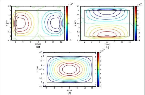
The displacement vector profiles of the fundamental trans-verseU11Xacoustic mode are shown in Fig.3. It can be observed that for any transverse acousticUmnX mode with a dominantUX
component, have half sine-wave spatial variation of (m,n), but its non-dominantUYandUZcomponents have spatial variations
of (m+1,n+1) and (m+1,n), respectively.
(b)
(c) (a)
k = 17 umI -1 W = 6 um, H = 3 umI I 9 8.5 8 7.5 7 6.5 6 5.5 5 4.5 4
4 5 6 7 8 9 10 11 12 0
1 2 3 4 5 6 7 8 9x10 3 _
k = 17 umI -1 W = 6 um, H = 3 umI I
_ 2.5 x10⁴ _ 2.5 2 1.5 1 0.5 0 0.5 1 1.5 2 _ _ _ _
4 5 6 7 8 9 10 11 12
9 8.5 8 7.5 7 6.5 6 5.5 5 4.5 4
k = 17 umI -1 W = 6 um, H = 3 umI I 6 x10⁶ _ 8 6 4 2 0 2 4 _ _ _ _
4 5 6 7 8 9 10 11 12
9 8.5 8 7.5 7 6.5 6 5.5 5 4.5 4 X (µm) Y (µm) X (µm) Y (µm) X (µm) Y (µm)
Fig. 3.Displacement vector profiles (a)UX, (b)UYand (c)UZ
of the fundamental transverseUX
11acoustic mode.
This waveguide can also guide longitudinal acoustic modes as the cladding longitudinal velocity is also higher than that of the core. The variations of the phase velocities of the fundamen-tal and higher order longitudinal modes with the frequency are shown in Fig.4. When frequency is decreased gradually, the ve-locities of the modes increase from near core velocity to cladding longitudinal wave velocity until they reaches to their cut-off when changes are rapid. The variations of the phase velocities of theU21Z andU12Z modes are shown by a red and a yellow lines, with diamond and rightward arrow, respectively and they are distinct. It can be observed that the red line lies below the yellow line for the whole range of the acoustic frequency considered here as the guide width was larger than the height. Here it can also be observed that a higher order mode reaches its cut-off at a higher frequency.
It was observed that the spatial variations of the displacement vector profiles of the longitudinal acoustic modes are different from those of the transverse modes. The dominant and non-dominant displacement vector profiles of the fundamental lon-gitudinal,U11Z mode are shown in Fig.5. It can be observed that itsUZprofile has one (m= 1) half-sine variation along thexand
similarly one (n= 1) half-sine variation along they-directions. On the other hand, theUXprofile of thisU11Z mode has one
[image:4.612.46.303.376.523.2]0 5 10 15 20 25 30 5500 5550 5600 5650 5700 5750 5800 5850 5900 Frequency (GHz) Longitud inal Ph ase V elocity (m /s)
UZ11
UZ21
UZ12
UZ31
UZ22
UZ41
[image:5.612.312.572.91.239.2]UZ32
Fig. 4.Variations of the phase velocities with the acoustic fre-quencies for the longitudinal modes.
X (µm) Y ( µ m )
5 6 7 8 9 10 11
4.5 5 5.5 6 6.5 7 7.5 8 8.5 0 1 x 10 2 4 _ X (µm) Y ( µ m )
5 6 7 8 9 10 11
4.5 5 5.5 6 6.5 7 7.5 8 8.5 0 1 2 3 4 5 6 7 x 10 8 _4 X (µm) Y ( µ m )
5 6 7 8 9 10 11
[image:5.612.42.300.112.256.2]−4 −3 −2 −1 0 1 2 3 4 5 x 10_ 4 8.5 8 7.5 7 6.5 6 5.5 5 4.5 (a) (b) (c) −2 −1
Fig. 5.Displacement vector profiles (a)UX, (b)UYand (c)UZ
of theU11Z acoustic mode.
Modal solutions of the optical waves in silica planar waveg-uide, for a wavelengthλo= 1550 nm, are obtained by using a
full-vectorialH-field formulation [15]. Here refractive indices of core and cladding are taken as 1.459 and 1.444, respectively. Both quasi-TE and quasi-TM modes can exist in this waveguide, but they have similar propagation constants and the profiles of their dominantH-fields are also similar. In this paper the interaction of the transverse and longitudinal acoustic modes with the fundamental quasi-TE,HY
11mode are studied. At first
the effect of waveguide dimensions on the modal properties of both optical and acoustic modes are studied. However, as in most of the planar optical waveguides often the guide widths are easily controlled by mask design for a given planar thickness, so here only the effect of width is shown. The variations of the effective index(ne f f)and effective area(Ae f f)of theH11Y mode
with the guide width (W) are presented in Fig. 6by a dashed blue and a red solid lines, respectively. The mode size area or the effective area(Ae f f)can be given [23] by,
Ae f f = R R
Ω|Et|2dxdy2 R R
Ω|Et|4dxdy
(10)
[image:5.612.42.298.302.469.2]2.0 3.0 4.0 5.0 6.0 7.0 8.0 9.0 10.0 11.0 1.446 1.447 1.448 1.449 1.450 1.451 20 22 24 26 28 30 32 34 36 38 W ( nef f Aef f neff Aeff (µm ) 2
Fig. 6.Variations of thene f f andAe f f of theHY11mode with
the guide width, W.
It can be observed that as the waveguide width, W, is re-duced, initially the effective area,Ae f f, reduces and reaches its
minimum value of 26.37µm2when W = 4µm. However, if W is
reduced further, its effective area increases rapidly as the optical mode approaches its effective cut-off condition. Moreover, when the guide width reduces,ne f f gradually falls from the effective
index of a slab with height (H) 3µm, to the cladding refractive
index value. Below a width of 4µm, the optical mode spreads
out before reaching its cut-off. It should be noted that as modes spreads out more from the core into the cladding, the scattering loss at the core-cladding interface, leakage loss, and bending loss (if bent), increase rapidly and it cannot be used as an effective waveguide.
In a way similar to the optical mode, the acousticUXvector
profile of the acousticU11X mode also varies with the waveguide width. The variations of the spotsizes along thexandy direc-tions with the width, W, for theUXprofile, when propagation
constantk= 12µm−1, are shown in Fig. 7. In this work, the
acoustic spotsize is considered as the distance along thexand
y-axes where the acoustic displacement profile is approximately equal to the 1/etimes of the maximum value of a given acoustic mode. Here, the guide height is kept constant at H = 3µm. The
spotsize,σX, denoted by a blue dashed line, decreases as the
width is decreased but near the effective cut-off this value start increasing. The spotsize, σY, remains almost constant (as the
height was kept constant) as guide width decreases but only near the cut-off, where the spotsize,σY, increases.
The frequency and the intensity of the backward flow of the pump signal, termed the Stokes wave, depends essentially on the phase and momentum matching and the overlap between, respectively, the acoustic and optical waves. This phenomenon is further stimulated when interference occurs between the Stokes wave and the laser signal and this strengthens the acoustic wave through electrostriction. Since the scattered light undergoes a Doppler frequency shift, the SBS frequency, fSBS, depends on
the acoustic velocity and this can be calculated [1,24] from,
fSBS=
2ne f fv
λo (11)
here,vis the acoustic velocity,λois optical wavelength andne f f
0 1 2 3 4 5 6 7 8 9 10 0
1 2 3 4 5 6 7 8 9 10
W (µm)
Spotsize of U in U (µm)
X
11
X X
Y H = 3 µm
[image:6.612.45.307.34.193.2]k = 12 µm_1
Fig. 7.Variation of spotsizes of theUXprofile for theU11X
mode with the width, W.
The dominantHYfield profile of the quasi-TE mode has
simi-lar profile to that of the dominantUX,UYandUZvector fields of
the fundamentalU11X,UY11andU11Z acoustic modes, respectively. The normalized amplitude variations of these profiles alongx -axis for W = 6µm, H = 3µm,λo= 1.55µmandk= 11.75µm−1
are shown in Fig. 8. Thekvalue selected here is the required propagation constant of the acoustic modes phase matched to quasi-TE optical mode atλo = 1.55µm. TheUX,UYandUZ
displacement vector profiles are almost identical and they were difficult to identify individually. TheHYprofile of the quasi-TE
mode atλo= 1550 nm is also shown by a solid black line in Fig. 8, which spreads more into the cladding region, compared to the acoustic mode profiles for this specific case.
0 2 4 6 8 10 12 14 16 18
0 2 0 0.2 0.4 0.6 0.8 1 1.2
Ampl
itude
HY 11 UX
11 UY 11 UZ 11 W = 6
k = 11.75372 1
W
[image:6.612.317.578.35.188.2]µ
Fig. 8.Normalized field and displacement vector profiles along thex-axis.
Next, the overlap between the fundamental longitudinal,UZ
11
acoustic mode and theH11Y optical mode is calculated when varying the waveguide width and this is shown in Fig.9by the dashed blue line. When the guide width increases, the overlap increases more prominently at the beginning then reaches near to its maximum overlap value, after which it increases slowly. The overlap found at 10µmwidth was 94%.
As expected, the overlap ofUZdisplacement vector of the
UZ
21 mode (with odd profile) with the HY field of HY11 mode
(with even profile) was calculated to be zero and not shown here.
2 3 4 5 6 7 8 9 10 11
0.80 0.82 0.84 0.86 0.88 0.90 0.92 0.94 0.96 0.98 1.00
0.000 0.005 0.010 0.015 0.020 0.025 0.030
W(µm)
(Overlap)
of U
Z 11
(Overlap)
of U
Z 31
Overlap of U with H11Z
Y 11
Overlap of U with HZ31
[image:6.612.55.290.393.579.2]Y 11
Fig. 9.Overlap ofHYfield of theHY11mode with theUZ
dis-placement vector of theU11Z andU31Z modes with W.
Following this, the overlaps of the dominantH11Y optical field with the higher order longitudinalU31Z acoustic mode but with symmetric (or even) displacement profiles is also determined and the overlap variation with the width is shown by a solid (red) line in Fig. 9. With the increase in the guide width, as the mode profile becomes more confined, the overlap decreases. It can be noted that, for this mode, the maximum overlap was found to be near 2.5%, at the lower guide width.
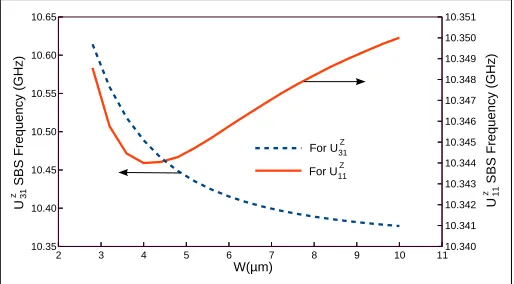
After determining the propagation constant,βo, of the
inter-actingH11Y mode, the propagation constant of the acoustic mode can be found using Eq. (8). The corresponding phase velocity,
v, of the acoustic mode can then be determined and thus Eq. (11) can yield the SBS frequency. In Fig.10, the SBS frequency shifts with the guide width for the fundamental longitudinal acoustic mode,U11Z, and the third order longitudinal,U31Z mode are shown by a solid red and a dashed blue lines, respectively. Here the dashed blue line falls with the increasing guide width, whereas the solid red line reaches its minimum near the 4µm
width and rises again with the increase of width, although this variation is, very small, when compared to the variation for the higher order longitudinalU31Z mode.
2 3 4 5 6 7 8 9 10 11
10.35 10.40 10.45 10.50 10.55 10.60 10.65
10.340 10.341 10.342 10.343 10.344 10.345 10.346 10.347 10.348 10.349 10.350 10.351
W(µm)
U SBS Fre
quency (GHz)
z 31
For U11Z
For U31Z
U SBS Fre
quency (GHz)
z 11
Fig. 10.SBS frequency shifts for theU11Z andU31Z modes with waveguide width.
[image:6.612.321.578.484.626.2]be larger than that of a longitudinal mode, where the numeri-cal results were verified experimentally and in the numerinumeri-cal analysis molecular displacements were considered rather than density variation, as done in this work.
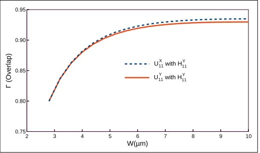
As the field profiles of both the dominating fields of the acous-tic transverse modes are similar to theHYfield profile of theH11Y
mode, their overlap was found to be quite high. Such overlaps can be calculated by using the normalized form of Eq. (9) and shown in Fig. 11. It can be observed from this figure that the overlap of theUXfield profile of dominant fundamental
acous-tic transverse modeUX
11 with theHYfield profile of quasi-TE
mode becomes higher when the guide width is wider. At a larger guide width, theUXfield profile ofU11Xbecomes more elongated
and this profile becomes closer in shape to the optical profile. Furthermore, it can be noted that the change of the overlap be-tween theUYdisplacement profile of theUY11mode andHYfield
profile with the guide width is slightly less than the overlap for theU11X mode as shown here and both of them are considerably lower than that of theUZ
11mode, which was shown in Fig.9.
2 3 4 5 6 7 8 9 10
0.75 0.80 0.85 0.90 0.95
W(µm)
(Overlap)
U with H11X Y 11
[image:7.612.314.572.100.249.2]U with HY11 Y 11
Fig. 11.Variations of theHYfield overlap of theH11Y mode
with theU11X andU11Y modes with the width.
Figure12shows the value offSBSfor the both fundamental
acousticU11XandU11Y transverse modes. The SBS frequency shift for theUX
11 mode shown by a dashed blue line in Fig. 12is
slightly lower than the SBS frequency shift denoted by red solid line for theU11Y mode. When the width increases from 2.8µmto
10µm, its optical effective index increases by 0.266%, while its
phase matched acoustic velocity reduces by 0.337%. However, as the dispersion curves are not linear, this yield a minimum SBS frequency shift between 4-5µm. In general, the total ranges of
variation of the values of fSBSfor both the fundamental
trans-verse modes are quite small (as the numerical values of the changes are only seen in the third digit after the decimal point). It can be noted that for any existing optical mode, when the guide width (W) increases the optical propagation constant(βo)
also increases. Asβoincreases, to maintain the phase matching,
the acoustic propagation constant (k) also increases according to Eq. (8). Moreover, for any given waveguide the acoustic frequency increases with the incrementing ofk. However, as the width also increases, due to these cumulative variations the result is the profile of the SBS frequency with the width which
2 3 4 5 6 7 8 9 10
6.523 6.524 6.525 6.526 6.527 6.528 6.529
Shear
SBS
Freque
ncy (GHz)
UX11
W ( m) U11Y
Fig. 12.SBS Frequency shift with guide width.
2 3 4 5 6 7 8 9 10 11
6.52 6.53 6.54 6.55 6.56 6.57 6.58 6.59
0.07 0.09 0.11 0.13 0.15 0.17 0.19 0.21
SBS Frequency Overlap
W(µm)
(Overlap)
SBS
Freque
ncy (GHz) for U
[image:7.612.314.570.283.430.2]X 21
Fig. 13.SBS frequency and overlap for theUZcomponent of
theU21Xmode with varying guide width.
As the dominantHY field profile of theH11Y mode and the
dominant displacement profiles of the fundamental acoustic modes are similar, their overlaps would be significant, as shown in Fig.11. On the other hand, the overlap of thisHYfield
pro-file of the quasi-TE mode with the non-dominant displacement vector profiles of the fundamental acoustic longitudinal and transverse modes, which have odd symmetry, will cancel out and the resulting acousto-optical interactions would be negligi-ble. However, it is expected that the maximum overlap of theHY
field profile with the dominantUXprofile of theU31Xmode will
be small, and this was observed to be around 3.5% (but is not shown here). However, it should be noted that although the over-lap ofUXprofile of theU21Xmode with the optical field is zero as
the former has odd symmetry, however the non-dominantUZ
profile of this mode may have a considerable overlap, as this dis-placement vector profile has an even symmetry. The variations of the overlap ofUZfield profile ofU21X mode with the width
is shown in Fig.13by a red solid line, where it increases along with the guide width. It is observed that the non-dominant
UZfield profile ofU21X mode has a near 20% overlap with the
[image:7.612.42.300.325.477.2]increasing width. Previously it was also observed, in Fig. 10, that for theU31Z longitudinal mode the value offSBSalso reduces
with the width, but had higher values as its longitudinal and shear velocities were higher.
Another important parameter, the peak Brillouin gain,gB,
can be calculated according to [26]:
gB=Γ
4πn8p212 λ3ocρfSBS4vB
(12)
where,Γis acousto-optical overlap,nis refractive index of the core,p12is elasto-optic coefficient,λois wavelength of the pump,
ρis density of silica, fSBSis Brillouin frequency shift,cis speed
of light in free space and4vBis the Brillouin gain linewidth.
Before calculation of the Brillouin gain coefficients, it is im-portant to estimate these parameters for 10% Ge-doped silica waveguide. The Brillouin gain linewidth,4vBis related to the
lifetime (TB) of phonon, i.e. the quanta of acoustic vibration, in
the material. It is the full-width at half-maximum (FWHM) of the Lorentzian gain profile [27]. The spectral width can be re-lated to the damping time of acoustic wave by [28]4vB = π1TB.
For 10% Ge-doped silica if the acoustic wave damping time is considered asTB = 6.469ns[29], then we have,4vB= 49.205
MHz. For such a structure, often it is assumed that4vBto be
equal for all acoustic modes and is assumed to be around 30-50
MHzfor all silica based fibers [27]. The value of 49.205 MHz
is used as Brillouin gain linewidth for all the acoustic modes of this structure.
The another important parameter is thep12, the elasto-optic
coefficient. Its value for 3.6% Ge-doped silica with refractive index,n= 1.4492, is 0.27 [30]. This value was considered for optical wavelengthλo= 1550nm. For silica, the value ofp12=
0.286 [26]. It is well known that for binarySiO2-GeO2glass
the refractive index has a nearly linear relationship with molar composition. It was also reported [31] that for aluminosilicate optical fiberp12shows a linear relation with the concentration of
alumina in silica. For the un-doped and 3.6% Ge-doped silica the
p12values have been reported as of 0.286 and 0.27, respectively,
and from these values, thep12value for 10% Ge-doped silica can
be extrapolated as 0.2416.
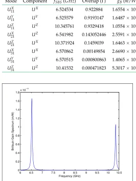
At the phase matched conditionΓandfSBScan be calculated
from Eqs. (9) and (11), respectively as shown earlier. Subse-quently using Eq. (12), the Brillouin gain coefficient for the 10% Ge-doped silica waveguide can also be calculated for fundamen-tal and higher order acoustic waves. Table1provides overlaps, Brillouin gain coefficients, SBS frequencies and corresponding acoustic velocities of the transverse and longitudinal acoustic modes at the phase matchedk= 11.75372µm−1. Among the
fun-damental and higher order acoustic transverse and longitudinal modes, which have considerable contributions in Brillouin gain spectrum are only considered here. Other acoustic modes for be-ing odd symmetric will either cancel out or may have negligible gain.
The frequency dependent Brillouin gain,gB(f), for an
indi-vidual mode has a Lorentzian spectral profile and can be given as [24]:
gB(f) =gB
(4vB/2)2
(f−fSBS)2+ (4vB/2)2
(13)
where,gBis the Brillouin gain peak, fSBSis Brillouin frequency
shift, and4vBis Brillouin gain linewidth.
The Brillouin gain spectrum (BGS) for 10% Ge-dopoed silica are obtained by considering the gain spectra due to various acoustic modes are statistically independent [27]. The BGS for
the 10% Ge-doped silica waveguide in between 6 to 10.5GHzis shown in Fig.14. There are two significant peaks observed, the fist peak is the contribution ofU11XandUY11modes and the second peak caused byUZ
11andU21Z modes. Due to comparatively larger
value of the linewidth, the peaks of two fundamental transverse
UX
11andU11Y modes are not distinguishable. It can also be noted
[image:8.612.317.583.198.552.2]that in this case, the gain peak for the transverse mode is higher than that of the longitudinal mode, similar as reported earlier [25].
Table 1.Overlaps and Brillouin gain coefficients for trans-verse and longitudinal fundamental and higher order acous-tic modes
Mode Component fSBS(GHz) Overlap (Γ) gB(m/W)
UX
11 UX 6.524534 0.922884 1.6554×10⁻¹¹
U11Y UY 6.525579 0.9193147 1.6487×10⁻¹¹
UZ
11 UZ 10.345761 0.9329418 1.0554×10⁻¹¹
U21X UZ 6.541982 0.143052446 2.5591×10⁻¹²
UZ
21 UX 10.371924 0.1459039 1.6463×10⁻¹²
U31X UX 6.570862 0.00149854 2.6690×10⁻¹⁴
U31Y UY 6.570515 0.000800863 1.4065×10⁻¹⁴
U31Z UZ 10.41532 0.000471823 5.3017×10⁻¹⁵
6 6.5 7 7.5 8 8.5 9 9.5 10 10.5 0
0.2 0.4 0.6 0.8 1 1.2 1.4 1.6 1.8x 10
−11
Frequency (GHz)
Brillouin Gain Spectrum (m/W)
Fig. 14.Brillouin gain spectrum of 10% Ge-doped silica waveguide between 6 GHz to 10.5GHz.
4. CONCLUSION
and transverse acoustic modes with the fundamental quasi-TE optical mode.
It was observed that all the acoustic modes are hybrid in nature with all the three components of the displacement vectors. It was also shown that the non-dominant displacement vectors have smaller magnitudes but also have higher order spatial variations. Further, it was observed that for the fundamental acoustic modes (for both longitudinal and transverse modes) the overlap of the non-dominant displacement vectors (being anti-symmetric) with the dominantHYprofile (of the fundamental
quasi-TE mode) is zero.
For the first time, it was also shown here that the non-dominant displacement vector of higher order acoustic modes can have a symmetric profile and also a considerably higher over-lap with the optical mode. It has also been shown in this work that although the overlap of the dominant displacement vector of a mode with odd spatial variations was zero with the fun-damental quasi-TE mode, but the overlap of its non-dominant displacement vector was significantly high and cannot be ig-nored.
The Brillouin gain coefficients of some transverse and longi-tudinal modes are also calculated and presented. Along with these the Brillouin gain spectrum from 6GHzto 10.5GHzis presented, which shows larger two peaks around 6.524534GHz
and 10.345761GHz.
A rigorous study of light-sound interactions in optical waveg-uide can be useful in the development of novel SBS sensors or in the design of optical waveguide to deliver high power. Thus the research presented has shown that to study light-sound inter-action in an effective way, the use of full-vectorial acoustic and optical modal approaches are necessary.
REFERENCES
1. G. P. Agrawal,Nonlinear Fiber Optics, 5th ed. (Academic Press, 2013). 2. K. Park and Y. Jeong, “A quasi-mode interpretation of acoustic radiation modes for analyzing Brillouin gain spectra of acoustically antiguiding optical fibers,”Opt. Exp.22(7), 7932–7946 (Apr. 2014).
3. B. A. Auld,Acoustic Fields and Waves in Solids, vol. I (John Wiley & Sons, 1973).
4. P. Dainese, P. St. J. Russell, N. Joly, J. C. Knight, G. S. Wiederhecker, H. L. Fragnito, V. Laude and A. Khelif, “Stimulated Brillouin scattering from multi-GHz-guided acoustic phonons in nanostructured photonic crystal fibers,”Nature Phys.2, 388–392 (Jun. 2006).
5. R. N. Thurston, “Elastic waves in rods and clad rods,”J. Acous. Soc. Am.
64(1), 1–37 (Jul. 1978).
6. A. Saffaai-Jazi, “Acoustic modes in optical fiber like waveguides,”IEEE Trans. Ultrason. Ferroelectr. Freq. Control35(5), 619–627 (Sep. 1988). 7. B. M. A. Rahman, M. M. Rahman, S. Sriratanavaree, N. Kejalakshmy, and K. T. V. Grattan, “Rigorous analysis of the transverse acoustic modes in optical waveguide by exploiting their structural symmetry,”App. Opt.
53(29), 6797–6803 (Oct. 2014).
8. B. M. A. Rahman and A. Agrawal,Finite Element Modelling Methods for Photonics(Artech House, 2013).
9. M. Koshiba, S. Mitobe, and M. Suzuki, “Finite-element solution of peri-odic waveguides for acoustic waves,”IEEE Trans. Ultrason. Ferroelectr. Freq. ControlUFFC-34(4), 472–477 (Jul. 1987).
10. P. E. Lagasse, “Higher-order finite-element analysis of topographic guides supporting elastic surface waves,”J. Acoust. Soc. Am.53(4), 1116–1122 (Jan. 1973).
Opt. Exp.22(8), 9528–9536 (Apr. 2014).
13. B. Ward and J. Spring,“Finite element analysis of Brillouin gain in SBS-suppressing optical fibers with non-uniform acoustic velocity profiles,”
Opt. Exp.17(18), 15685–15699 (Aug. 2009).
14. O. C. Zienkiewicz, R. L. Taylor, and J. Z. Zhu,The Finite Element Method: Its Basis and Fundamentals, 7th ed. (Butterworth-Heinemann, 2013).
15. B. M. A. Rahman and J. B. Davies, “Finite element solution of integrated optical waveguides,”J. Lightwave Technol.LT-2(5), 682–688 (Oct. 1984). 16. R. W. Boyd,Nonlinear Optics, 3rd ed. (Academic Press, 2008). 17. P. T. Rakich, C. Reinke, R. Camacho, P. Davids, and Z. Wang,“Giant
enhancement of stimulated Brillouin scattering in the subwavelength limit,”Phys. Rev. X2, 011008(1–15) (Jan. 2012).
18. L. Tartara, C. Codemard, J. -N. Maran, R. Cherif and M. Zghal, “Full modal analysis of the Brillouin gain spectrum of an optical fiber,”Opt. Comm.282(12), 2431–2436 (Jun. 2009).
19. R. Pant, C. G. Poulton, D. -Y. Choi, H. Mcfarlane, S. Hile, E. Li, L. Thevenaz, B. L. -Davies, S. J. Madden and B. J. Eggleton,“On-chip stimulated Brillouin scattering,”Opt. Exp.19(9), 8285–8290 (Apr. 2011). 20. M. -J. Li, X. Chen, J. Wang, S. Gray, A. Liu, J. A. Demeritt, A. B. Ruffin, A. M. Crowley, D. T. Walton, and L. A. Zenteno, “Al-Ge co-doped large mode area fiber with high SBS threshold,”Opt. Lett.15(13), 8290–8299 (Jun. 2007).
21. C. K. Jen, A. Saffaai-Jazi, and G. W. Farnell, “Leaky modes in weakly guiding fiber acoustic waveguides,”IEEE Tran. Ultrason. Ferroelectr. Freq. ControlUFFC-33(6), 619–627 (Nov. 1986).
22. P. D. Dragic, “The acoustic velocity of Ge-doped silica fibers: A compar-ison of two models,”Int. J. App. Glass Sci.1(3), 330–337 (Aug. 2010). 23. M. Uthman, B. M. A. Rahman, N. Kejalakshmy, A. Agrawal, H. Abana,
and K. T. V. Grattan, “Stabilized large mode area in tapered photonic crystal fiber for stable coupling,”IEEE Photon. J.4(2), 340–349 (Apr. 2012).
24. M. Nikles, L. Thevenaz, and P. A. Robert, “Brillouin gain spectrum characterization in single-mode optical fibers,”J. Lightwave Tech.15(10), 1842–1851 (Oct. 1997).
25. J. -C. Beugnot, S. Lebrun, G. Pauliat, H. Maillotte, V. Laude and T. Sylvestre, “Brilllouin light scattering from surface acoustic waves in a subwavelength-diameter optical fiber,”Nat. Comm.5(5242), 1–6 (Oct. 2014).
26. B. J. Eggleton, C. G. Poulton and R. Pant, “Inducing and harnessing stimulated Brillouin scattering in photonic integrated circuits,”Adv. Opt. Phot.5, 536–587 (Dec. 2013).
27. S. Dasgupta, F. Poletti, S. Liu, P. Petropoulos, D. J. Richardson, L. Gru¨ner-Nielsen and S. Herstrom, “Modelling Brillouin gain spectrum of solid and microstructured optical fibers using a finite element method,”J. Lightwave Tech.29(1), 22–30 (Jan. 2011).
28. K. Ogusu and H. Li, “Brillouin-gain coefficient of chalcogenide glasses,”
J. Opt. Soc. Am. B21(7), 1302–1304 (Jul. 2004).
29. Y. Koyamada, S. Sato, S. Nakamura, H. Sotobayashi and W. Chujo, “Simulating and designing Brillouin gain spectrum in single-mode fibers,”
J. Lightwave Tech.22(2), 631–639 (Feb. 2004).
30. J. -C. Beugnot and V. Laude, “Electrostriction and guidance of acoustic phonons in optical fibers,”Phys. Rev. B86(22), 224304 (Dec. 2012). 31. P. D. Dragic, J. Ballato, S. Morris and T. Hawkins, “Pockel’s coefficient