Does software have to be ultra reliable in safety critical systems?

City, University of London Institutional Repository

Citation:

Bishop, P. G. (2013). Does software have to be ultra reliable in safety critical

systems?. Paper presented at the SAFECOMP 2013, 32nd International Conference on

Computer Safety, Reliability and Security, 24 - 27 September 2013, Toulouse, France.

This is the unspecified version of the paper.

This version of the publication may differ from the final published

version.

Permanent repository link:

http://openaccess.city.ac.uk/2465/

Link to published version:

Copyright and reuse: City Research Online aims to make research

outputs of City, University of London available to a wider audience.

Copyright and Moral Rights remain with the author(s) and/or copyright

holders. URLs from City Research Online may be freely distributed and

linked to.

City Research Online:

http://openaccess.city.ac.uk/

publications@city.ac.uk

Systems?

Peter Bishop1,2

1

Centre for Software Reliability, City University, London, EC1V 0HB, UK

pgb@csr.city.ac.uk

2

Adelard LLP, London, Exmouth House, London,, EC1R 0JH, UK

pgb@adelard.com

Abstract—It is difficult to demonstrate that safety-critical software is com-pletely free of dangerous faults. Prior testing can be used to demonstrate that the unsafe failure rate is below some bound, but in practice, the bound is not low enough to demonstrate the level of safety performance required for critical software-based systems like avionics. This paper argues higher levels of safety performance can be claimed by taking account of: 1) external mitigation to pre-vent an accident: 2) the fact that software is corrected once failures are detected in operation. A model based on these concepts is developed to derive an upper bound on the number of expected failures and accidents under different assump-tions about fault fixing, diagnosis, repair and accident mitigation. A numerical example is used to illustrate the approach. The implications and potential appli-cations of the theory are discussed.

Keywords. safety, software defects, software reliability, fault tolerance, fault correction.

1

Introduction

It is difficult to show that software has an acceptably low dangerous failure rate for a safety-critical system. The work of Butler and Finelli [4] and Littlewood and Strigini [21] suggests that there is a limit on the rate that can be demonstrated by testing. Given the difficulty of testing the software under realistic conditions, it is often claimed that this limit is likely to be around 10−4 to 10−5 failures per hour [18]. As these tests would typically be completed without any failures, we do not know what proportion of the failures are likely to be dangerous, so we have to use the bound derived from testing as the upper bound for the dangerous failure rate as well.

civil jet airliners world-wide, around 500,000 fatal aircraft accidents could occur every year. In practice, statistics on aircraft accidents [2] show that there are around 40 airliner accidents per year worldwide from all causes (including pilot error).

It is clear that real avionics systems perform far better than we are entitled to ex-pect based on testing alone [25], but the actual performance can only be determined

after the system has been deployed. What we need is a credible argument that would

convince a regulator that a software-based system is suitable for use in a safety-critical context before it is deployed in actual operation [11].

One alternative to empirical test evidence is the claim that compliance to estab-lished standards for safety-critical software will result in software with a tolerable dangerous failure rate. For example, compliance to IEC 61508 Level 4 is linked with dangerous system failure rates as low as 10-9/hr [9]. Unfortunately there is very little empirical evidence to support such a claim.

More credibly, it may be possible to support a claim of perfection if the software is proved correct using formal methods [8]. In this case any failure rate target, even a stringent target like 10-9 per hour, would be achievable and the Probabilistic Safety Assessment (PSA) of the overall system could assume the software had a dangerous failure rate of zero. In practice however, few systems have been constructed using formal proof methods, and even these systems cannot be guaranteed to be fault free (e.g. due to errors in requirements or faults in the proof tools [6, 20]).

Another alternative is a risk-informed based design approach [19] which focuses on reducing dangerous failure modes rather than seeking software perfection. Poten-tially hazardous failure modes are identified and safeguards against these failures are included in the design. However there is no guarantee that a hazard-based approach will identify all potential hazards in the real-world environment, and a convincing safety argument would need to show that the hazard identification is complete.

Safety assurance can also be achieved by the use of fault tolerance techniques [1], [14] like design diversity [22] that mitigates failures from individual software compo-nents. Software design diversity can reduce the dangerous failure rate of the compos-ite system as the same failure has to occur in more than one software component be-fore it becomes dangerous. These techniques have been used in a range of safety-critical systems [3, 15].

It should be noted that all these strategies for producing safe software are vulner-able to an error in the original specification, i.e. when there is a mismatch between the software requirement and the real world need. This unfortunately also limits the po-tential for accelerated testing of software against the requirement to reduce the dan-gerous failure rate bound as the tests will omit the same key features of real-world behaviour.

In practice, systems designers use the defence-in-depth principle to mitigate the impact of dangerous failures in subsystems [7, 10, 20], for example,

• A nuclear protection system failure is covered by an independently designed sec-ondary protection system, manual shutdown and post incident control measures. • A flight control system failure is covered by diverse flight controls and pilot

As a result of these strategies, the dangerous failure rate of the system function can be lower than that of any individual software component. This can be formalized as:

λ

λ

=

p

where λacc is the accident rate, pacc is the probability that a dangerous subsystem

fail-ure will cause an accident and λ is the bound on the dangerous software failfail-ure rate established by testing.

The problem lies in achieving and justifying an appropriate value of pacc. Empirical

studies of software fault tolerance techniques like design diversity [16, 26] suggest that reductions of no more than two orders of magnitude can be achieved, while hu-man intervention under stress may only result in another order of magnitude reduction in the dangerous failure giving a total reduction of 10−3. If a dangerous failure rate of

10−4/hr can be demonstrated from actual flight testing, it might be argued that the accident rate due to failure of the avionics subsystem is no worse than 10−7/hr, but this could still be insufficient to demonstrate the required target (e.g. 10−9/hr for an avion-ics function).

In this paper we will present a probabilistic software failure model that can be used to claim a lower contribution to the accident rate from dangerous software faults. This approach is novel and potentially controversial as it requires certification bodies to accept an argument based on a low average risk over the system lifetime, but with the possibility of a higher instantaneous risk when the system is first introduced.

2

Basic Concept

Software failures need to be handled in a different way to hardware failures because a systematic software defect can be fixed—once we know what the problem is, it can be removed. In the best case, each software fault need only fail once if it is successfully fixed in all instances immediately after failure, so we consider that it is inappropriate to use a fixed failure rate for software in a safety justification. We also need to take account of the fact that software failures need not be catastrophic (i.e. cause an acci-dent), because there can be mitigations outside the software-based component.

In the most basic representation of this idea, we consider the failures caused by a single fault in the software (the impact of multiple faults will be considered later).

Clearly the number of failures that occur before the fault is successfully fixed de-pends on the probability of diagnosing a fault and then repairing it correctly [24]. In the basic model, we make the following assumptions.

• The conditional probability that a fault is diagnosed when a software failure occurs is pdiag.

• The conditional probability that a fault is repaired correctly after diagnosis is prepair.

• The success of diagnosis and repair is independent of the number of previous fail-ures.

Given the independence assumptions made on diagnosis and repair, the probability of a fault being successfully fixed after each failure is:

repair diag

fix

p

p

p

=

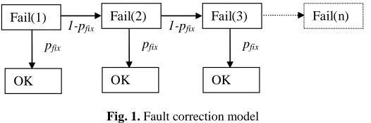
Given the assumption that no failures can occur during a fix, a simple transition model can be used to model the fixing process as illustrated in Fig 1.

Fail(1) OK pfix Fail(2) OK pfix 1-pfix Fail(3) OK pfix 1-pfix Fail(n)

Fig. 1. Fault correction model

So for pfix = 0.5, there is a 50% chance of removing a fault after the first failure; 25%

after the second failure; and so on. The mean length of this failure sequence, nfail, is:

∑

−

⋅

=

)

1

(

fail

n

p

p

n

Using a standard result for this geometric series [27], this reduces to:

fix fail

p

n

=

1

This represents the expected number of failures over an infinite period of time, caused by a single software fault operating within the whole fleet of software-based units. If there are N faults that cause dangerous failures, then the expected number of fleet failures due to these faults is bounded by:

fix fail

p

N

n

≤

The other element of the model is based on the fact that safety-related computer-based systems typically operate within a fault-tolerant architecture (as discussed earlier). We can represent this external mitigation of a dangerous software failure by the probabil-ity pacc that an accident occurs after a dangerous software failure.

It follows that the expected number of accidents over the lifetime of the fleet due to

N dangerous faults is bounded by:

fix acc acc

p

Np

This equation implies that if N<<pfix,/ pacc, the expected number of accidents nacc<<1.

This represents the case where there is a high probability that all N dangerous faults will be diagnosed and removed before the first accident occurs. A value of nacc well

below unity is effectively equivalent to the probability of an accident over the lifetime of the fleet due to failures of the software component.

Given the assumption that no further software failures occur during a fix attempt, the failure rate of the software has no impact on the maximum number of accidents in the fleet. This assumption could be satisfied if all failures resulted in an instantaneous fix attempt, or more realistically, it could be met if the fleet was grounded immedi-ately after failure while the fix attempt is made.

This independence between the upper bound on failure rate and the number of ac-cidents is particularly useful in cases where the failure rate bound has not been esti-mated correctly, e.g. due to a flaw in the specification. Such a flaw would invalidate any failure rate estimate based on testing, but the accident bound derived from equa-tion (6) would still be valid provided N included an estimate for dangerous specifica-tion flaws. This differs from hardware where the instantaneous failure rate is often assumed to be constant, so expected accidents always increase with fleet usage.

3

Impact of Delayed Fixing

The basic model makes a strong assumption that no further failures will occur after a dangerous failure is observed. In many cases however, the fleet containing the soft-ware components will continue to operate after the failure has occurred. Clearly, if repair is delayed, further failures could occur within the fault fixing interval.

Initially we will consider the case of a single fault (extension to N faults will be addressed later). Let us define:

λ as the upper bound on the software failure rate ∆tfix as the time needed to perform diagnosis and repair

τ(t) as the total execution time of the software fleet at elapsed time t

We further assume that:

• No new faults are introduced when the software is fixed.

• The failure rate bound λ is unchanged if the fix attempt is not successful.

These assumptions are also quite strong. New faults are known to occur occasionally but if the new fault is in the same defective code section, it can be modeled as the

same fault with a reduced pfix value.

To estimate the impact of delayed fixing, we first define the time needed before an average length failure sequence terminates, tfail,as the value that satisfies the equation:

fail fail

n

t

)

=

(

λτ

From equation (4), this is equivalent to:

fix fail

p

t

)

1

(

=

λτ

It can be shown using Jensen’s Inequality [17] that, if the execution time function τ(t) is convex (i.e. the gradient is constant or increases over calendar time), the total num-ber of failures, nfixedl, when the fix delay is included is bounded by:

)

(

fixed

t

t

n

≤

λτ

+

∆

We now consider a situation where there are N dangerous faults. Most reliability models assume the failures of the individual faults occur independently. If this as-sumption is made, the failure rates sum to λ, but we will take a worst case scenario where:

• The failure rate of each fault is λ.

• Failures occur simultaneously for N faults. • Only one fault can be fixed after a failure.

In this worst case scenario there will N times more failures than a single fault and the failures will occur at the same frequency, λ, as the single fault case. This failure se-quence is equivalent to having a single fault with a pfix probability that is N times

worse, i.e. where:

N

p

p

′

=

The bound in equation (9) can therefore be generalised to N faults as:

)

(

fixed

t

t

n

≤

λτ

′

+

∆

where:

fix fail

p

t

′

=

′

)

1

(

λτ

fix fail

p

N

t

′

)

=

(

λτ

It follows that the worst scale factor k due to delayed fixing, is:

)

(

)

(

t

t

t

n

n

k

′

∆

+

′

≤

=

τ

τ

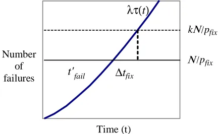
The basic principle for scaling the bound is illustrated in Fig 2. Without fixing, the expected number of failures increases to infinity. With fixing and no delay, the num-ber cannot exceed the basic bound, and would take a time t′fail for the bounding

num-ber of failures to occur. With a fix delay, the bound is increased to allow for the addi-tional failures that can occur in the extra time ∆tfixneeded for fault repair.

Time (t) Number

of

failures

t'

∆

t

λτ(

t

)

Ν

Ν

Fig. 2. Effect of fix delay on the expected number of failures

We can also compare the expected number of failures with fault fixing (nfixed) against

the expected number without fault fixing, (n unfixed), namely:

)

(

unfixed

t

n

=

λτ

where tfleet is the calendar time that the software is in operation in the fleet. So the

failure reduction (and hence accident reduction), r, achieved by fault fixing is:

)

(

)

(

t

t

t

n

n

r

τ

τ

′

+

∆

≤

=

t

′

+

∆

t

<

t

Application to Demand-based Systems. Equation (6) is directly applicable to any

For example, if we know there is an average demand rate of d demands per unit of execution time and the upper bound on the probability of failure on demand is f (e.g. from accelerated testing), the effective failure rate per unit of execution time is:

fd

=

λ

4

Theory Applied to an Avionics Example

To illustrate the potential gains achievable by including fault fixing, we will apply the theory to a hypothetical avionics example with the following parameters

c 10 unit sales per month

u 0.6 (fraction of time in use)

N 1

λ 10−4 failures/ hour

pfix 0.1 pacc 0.001

Note that the figures used are only estimates, but are considered to be realistic. The number of dangerous faults N is taken to be one as we assume thorough levels of testing and analysis (especially for the safe-critical portions of the software). The assumed failure rate represents a year of realistic flight testing (e.g. in ground based tests and actual test flights). The probability of an accident pacc is assumed to be small

because an aircraft is engineered to tolerate failures of specific components (via standby systems, pilot override, etc). The pfix probability is actually the product of

diagnosis and repair probabilities, i.e. pfix = pdiag⋅prepair. For critical software we expect

the repair probability achieved by the software support team to be close to unity, so

pfix is largely determined by the diagnosis probability, which is estimated to be around

0.1 as any hazardous incidents will occur in-flight, and diagnosis relies on later recon-struction of events based on in-flight recording data.

If the fleet is grounded after a dangerous failure, the basic model applies and we would expect 10 failures (from equation (3)) and 0.01 accidents (from equation (6)) over the fleet lifetime.

If there is delayed fixing, the k value has to be computed using the execution time equation. With a linear growth in the fleet of avionics units at c per month the execu-tion time funcexecu-tion can be shown to be:

2

2

)

(

t

=

cu

t

τ

We can use equations (13) and (14) and the execution time function (18) to com-pute the scale-up factor k. The impact of different fix delay times (∆tfix) on k and the

Table 1. Expected Accidents Over Infinite Time for Different Software Fix Times

∆tfix (months)

k

n

n

0 1 10 0.010

1 1.3 13 0.013

2 1.7 17 0.017

3 2.1 21 0.021

With a 3 month delay in fixing, the bound on the expected number of fleet accidents is only double the number predicted by the basic model (with no fix delay).

The upper bound on the mean accident rate λacc over the fleet lifetime is:

fleet acc acc

T

n

≤

λ

where Tfleet is the total execution time of all the avionics units.

From equation (18), if unit sales continued for 5 years, the total number of operat-ing hours, Tfleet, is around 1.6×107 hours. So the upper bound on the mean accident

rate λacc over the fleet lifetime for a 3 month fix delay is:

λacc ≤ 1.3×10-9 accidents per hour

This bound on the mean accident rate is close to the target of 10−9 accidents per hour required in avionics standards [12][13]. The bound could be reduced to less than 10−9 accidents per hour if a shorter fix delay is used (e.g. 1 month).

By comparison, if we only relied on external accident mitigation, the bound on the mean accident rate would be the same as the initial rate paccλ. For the avionics

exam-ple, the expected rate would be 1×10-7

accidents per hour.

So for this choice of model parameters, the inclusion of a fault removal model has reduced the expected accident rate over the fleet lifetime by two orders of magnitude. Clearly the reduction varies with the parameters used. Table 2 shows the accident reduction r achieved by fault fixing for different failure rates assuming a 3 month delay in fixing and a 5 year operating period.

Table 2. Accident Reduction for Different Software Failure Rates

Mean Accidents / hr λ

(per hr) _{(no fix) (fix)}

Reduction factor r

10−3 10−6 3.5×10−9 0.0035

10−4 10−7 1.3×10−9 0.013

10−5 10−8 0.8×10−9 0.08

5

Discussion

The fault fixing model predicts an upper bound on the total number of software fail-ures (and associated accidents) over the fleet lifetime. The impact of fault fixing is greatest in large fleets where the expected number of failures without fixing would greatly exceed the expected number with fault fixing. In the avionics example, the claimed accident rate can be two orders of magnitude less than would be predicted from testing alone. In particular, once a relatively modest (and demonstrable) level of software reliability is achieved, further reductions in failure rate make little difference to the ultimate number of failures and accidents.

This type of probabilistic argument is not currently accepted in safety standards or by certification and regulatory bodies. Early users of the system could be placed at greater risk if the instantaneous failure rate is close to the limit established by testing. However it might be more acceptable as a support to a primary argument such as a claim of zero faults in critical portions of the software. The supporting argument would be that, even if the claim of zero dangerous faults is invalid, there is high prob-ability that a software fault never causes any accident over the lifetime of the fleet (e.g. 98% in our avionics example).

If the theory is valid, equation (6) can also be helpful in choosing design trade offs. We note that an order of magnitude change in the predicted number of accidents can be achieved by an order of magnitude change in either: N, pdiag, or pacc. Knowing the

contribution of these parameters, design trade-offs can be based on cost and technical feasibility. For example, sending extra data to a shared black-box data recorder to improve pdiag might be more cost effective than additional effort to reduce N.

Alterna-tively installing a backup system using different technology might double the cost but improve pacc by orders of magnitude.

The theory also shows that the operational context can affect the accident probabil-ity. Obviously the repair probability pdiag directly affects the number of accidents, and

we can minimise the scale-up k due to delayed fixing by considering equations (13) and (14). For example k might be reduced by decreasing the fix delay time ∆tfix or by

reducing the growth in usage τ(t) for some trial period.

To successfully apply the model, evidence will be needed to show that the model parameter estimates are either realistic or at least conservative. Values, like N, could be derived from past experience with similar systems, (e.g. analysing FAA directives [5, 25]) but further research is needed on quantifying the model parameters.

More generally, the same theory should be applicable to any systematic design fault that is amenable to fault fixing such as software security vulnerabilities, hard-ware design faults or requirements faults.

6

Summary and Conclusions

failure rate. When this bound on failures is combined with external failure mitigation, there can be a high probability that an accident is never caused by dangerous software failure regardless of the size of the fleet using the software-based component.

We have also presented a refinement of the basic model that allows the bound to be increased to allow for a delay in fixing a detected fault. This revised bound is depend-ent on the software failure rate, but the increase is typically quite small.

The theory was illustrated by an aircraft avionics example where fault fixing re-duced the expected number of accidents by around two orders of magnitude over the fleet lifetime.

If the assumptions behind the theory are valid, it could provide an additional means of arguing that critical software-based systems are safe prior to deployment even though ultra high reliability of the software cannot be demonstrated by prior testing.

The theory might also be helpful in making design and support trade-offs to mini-mize the probability of an accident.

We also suggest that the theory could be applicable to any systematic fault (e.g. in requirements, hardware, software or mechanical components).

Further empirical research is recommended to validate the model assumptions and quantify the model parameters.

Acknowledgments. The author wishes to thank Bev Littlewood, Lorenzo Strigini,

Andrey Povyakalo and David Wright at the Centre for Software Reliability for their constructive comments in the preparation of this paper.

References

1. A Avizienis, J-C Laprie, B Randell; C Landwehr, “Basic concepts and taxonomy of de-pendable and secure computing”, IEEE Transactions on Dede-pendable and Secure

Comput-ing, , Vol. 1, Issue:1, pp. 11–33, Jan.-March 2004.

2. Boeing, “Statistical Summary of Commercial Jet Airplane Accidents Worldwide Opera-tions 1959 – 2010”, Aviation Safety, Boeing Commercial Airplanes, Seattle, Washington, U.S.A., June 2011.

3. D Briere and P Traverse, "Airbus A320/A330/A340 electrical flight controls — a family of fault-tolerant systems", Proc. 23rd IEEE Int. Symp. on Fault-Tolerant Computing (FTCS-23), pp. 616-623, June 1993.

4. RW Butler and GB Finelli, “The infeasibility of quantifying the reliability of life-critical real-time software”, IEEE Transactions on Software Engineering, vol. 19, no. 1, pp. 3-12, Jan. 1993.

5. FAA Airworthiness Directive database,

http://rgl.faa.gov/Regulatory_and_Guidance_Library/rgAD.nsf/MainFrame

6. PJ Graydon, JC Knight JC and Xiang Yin, “Practical Limits On Software Dependability: A Case Study”, 15th International Conference on Reliable Software Technologies –

Ada-Europe, June 2010.

7. H Hecht and M Hecht, “Software reliability in the system context”, IEEE Transactions on

Software Engineering. vol. 12, pp. 51-58. Jan. 1986.

9. IEC, Functional safety of electrical/electronic/programmable electronic safety-related

sys-tems, IEC 61508 ed. 2.0, International Electrotechnical Commission, 2010.

10. INSAG, Defence in Depth in Nuclear Safety, INSAG 10, International Nuclear Safety Ad-visory Group, 1996.

11. D Jackson, and M Thomas, Software for dependable systems: sufficient evidence?, Na-tional Research Council (U.S.). NaNa-tional Academic Press, ISBN 978-0-309-10394-7, 2007. 12. Joint Airworthiness Authority, Joint Airworthiness Requirements, Part 25: Large

Aero-planes, JAR 25, 1990.

13. Joint Airworthiness Authority, Advisory Material Joint (AMJ) relating to JAR 25.1309:

System Design and Analysis, AMJ 25.1309. 1990.

14. K Kanoun and J-C Laprie, “Dependability modeling and evaluation of software fault-tolerant systems”, IEEE Transactions on Computers, vol. 39, no. 4, pp. 504 – 513, 1990. 15. H. Kantz and C Koza, “The ELEKTRA Railway Signalling-System: Field Experience with

an Actively Replicated System with Diversity,” 25th IEEE Int. Symposium on

Fault-Tolerant Computing (FTCS-25), pp. 453-458, June 1995.

16. JC Knight and. NG Leveson, “An empirical study of failure probabilities in multi-version software.” in Digest. FTCS-16: Sixteenth Annual Int. Symp. Fault-Tolerant Computing, pp. 165- 170, July 1986.

17. SG Krantz, “Jensen's Inequality.” Section 9.1.3 in Handbook of Complex Variables. Bos-ton, MA: Birkhäuser, p. 118, 1999.

18. J-C Laprie, “For a product-in-a-process approach to software reliability evaluation”, Third

International Symposium on Software Reliability Engineering (ISSRE’92), pp. 134 – 139,

October 1992.

19. NG Leveson, Engineering a Safer World: Systems Thinking Applied to Safety, MIT Press, 2012, ISBN 978-0262016629.

20. B Littlewood and J Rushby, Reasoning about the Reliability of Diverse Two-Channel Sys-tems in Which One Channel Is "Possibly Perfect”, IEEE Transactions on Software

Engi-neering, Vol.: 38 , No: 5, pp. 1178 – 1194, 2012.

21. B Littlewood and L Strigini, “Validation of Ultra-High Dependability for Software-based Systems”, Communications of the ACM, vol. 36, no. 11, pp.69-80, Nov. 1993.

22. MT Lyu, Software Fault Tolerance, John Wiley & Sons, Inc. New York, SBN:0471950688, 1995.

23. Radio Technical Commission for Aeronautics, Software Considerations in Airborne

Sys-tems and Equipment Certification, RTCA/DO-178C. Washington, DC: RTCA, Dec. 2011.

24. C Smidts, “A stochastic model of human errors in software development: impact of repair times” Proceedings. 10th International Symposium on Software Reliability Engineering (ISSRE’99), pp. 94 – 103, 1999.

25. M Shooman. “Avionics Software Problem Occurrence Rates”, Seventh International

Sym-posium on Software Reliability Engineering (ISSRE’96), pp. 55-64, 1996.

26. MJP van der Meulen and MA Revilla, “The Effectiveness of Software Diversity in a Large Population of Programs”, IEEE Transactions on Software Engineering, vol. 34, no. 6, pp 753 – 764, Nov-Dec 2008.