Justin J. A. Conn, Brian R. Duffy, David Pritchard,∗ and Stephen K. Wilson
Department of Mathematics and Statistics, University of Strathclyde, 26 Richmond Street, Glasgow G1 1XH, Scotland, UK
Peter J. Halling
Department of Pure and Applied Chemistry, University of Strathclyde, 295 Cathedral Street, Glasgow G1 1XL, Scotland, UK
Khellil Sefiane
School of Engineering, University of Edinburgh, The King’s Buildings, Mayfield Road, Edinburgh EH9 3JL, Scotland, UK
(Dated: February 20, 2016)
We construct a fluid-dynamical model for the flow of a solution with a free surface at which surface tension acts. This model can describe both classical surfactants, which decrease the surface tension of the solution relative to that of the pure solvent, and ‘anti-surfactants’ (such as many salts when added to water, and small amounts of water when added to alcohol) which increase it. We demonstrate the utility of the model by considering the linear stability of an infinitely deep layer of initially quiescent fluid. In particular, we predict the occurrence of a novel instability driven by surface-tension gradients, which occurs for anti-surfactant, but not for surfactant, solutions.
I. INTRODUCTION
The surface tension of a solution generally differs from that of the pure solvent. The molecules or ions of many solutes accumulate preferentially at free surfaces, where they lower the surface tension [1]; such substances are consequently known as surfactants. However, it is also well known that there are other solutes that have the op-posite effect: as increasing amounts of these solutes are added to the solvent, the surface tension increases. Ex-amples include many salts when added to water [1, 2], and small amounts of water when added to alcohol [3]. For fluid-dynamical purposes, such solutes may conve-niently be described as ‘anti-surfactants’.
Since this anti-surfactant behaviour may play a signif-icant role in the flow of solutions with free surfaces, it is perhaps surprising that it has not yet been incorporated into fluid-dynamical models, especially as corresponding models for both soluble and insoluble surfactants are now well established and have been widely studied [4–8]. It should be noted that, in general, a model for an anti-surfactant cannot be obtained from one for a anti-surfactant simply by reversing the dependence of the surface ten-sion on the surface concentration of solute, because, as we shall explain below, this is not in general consistent with the underlying physical mechanisms by which so-lutes affect surface tension.
In this contribution we construct a fluid-dynamical model which builds on existing models for surfactants but which, unlike them, can also describe anti-surfactants. By considering a simple linear stability problem we demonstrate that the new model is tractable and predicts
∗Corresponding author: [email protected]
a novel instability driven by surface-tension gradients, which occurs for anti-surfactant, but not for surfactant, solutions.
II. MODEL CONSTRUCTION A. Bulk–surface flux and surface tension We follow many well-established fluid-dynamical mod-els of coupled flow and surfactant transport [4–8] by dis-tinguishing between the surface region of the fluid, taken to have a notional thicknessηof the order of ˚angstr¨oms, and the remaining bulk region of the fluid. The bulk re-gion may include a ‘subsurface’ rere-gion of high concentra-tion gradients, which mediates solute exchange between the surface and the deeper regions of the fluid [9]; for sim-plicity we assume that such a region may be described by the same governing equations as the rest of the bulk. The bulk concentration of solutecb is measured in mol m−3,
while the surface concentration of solutecs is measured
in mol m−2. The concentration in each region obeys an appropriate transport equation, and the exchange of so-lute between the bulk and the surface is described by the bulk–surface fluxJ measured in mol m−2s−1. When
the flux is zero, J = 0, the surface concentration is in equilibrium with the bulk concentration at the top of the bulk region; this is a good approximation when flow and transport processes are slow compared with the ki-netics of bulk–surface exchange. We will refer to this state as ‘bulk–surface equilibrium’, noting that a system that is in bulk–surface equilibrium may still be evolving slowly through diffusion-controlled adsorption [9–11]. In the more general situation in which the flux is non-zero,
some-times referred to as ‘mixed-kinetic adsorption’ [9]. It is usual in existing models of surfactants to treat the surface tensionσas a decreasing function of the sur-face concentrationcs. This approach was developed
orig-inally for insoluble surfactants [e.g. 4] and subsequently extended to soluble surfactants [e.g. 5–7]. However, as we shall see, in generalσ also depends on the bulk con-centrationcb evaluated at the top of the bulk region, or,
equivalently, on thesurface excessΓ, defined as
Γ =cs−ηcb, (1)
where again the concentrationcb is evaluated at the top
of the bulk region. The sign of Γ indicates whether the molecules of solute preferentially accumulate at the sur-face (Γ > 0), as they do for surfactants, or in the bulk (Γ<0), as they do for anti-surfactants. Note that when the surface concentration is high relative to the bulk con-centration (specifically, when cs ≫ηcb) the surface
ex-cess Γ is well approximated by cs, justifying the usual
approach for surfactants. However, as we shall now de-scribe, in general, and particularly for anti-surfactants, it is necessary to account for the dependence on cb, i.e.
to distinguish between Γ andcs.
Although the details of the electrochemical mecha-nisms that lead to the exclusion of particular species from the surface remain the topic of ongoing research [12, 13], the qualitative mechanism by which they affect the equi-librium surface tension is clear. Solvent molecules in the bulk interact with the dissolved solute; those near the surface have less interaction with the solute, as well as with other solvent molecules, and hence have higher en-ergy than in the bulk, the excess being exhibited as sur-face energy. What determines the net effect of the added solute is then not the absolute values ofcsandcb, but the
effective difference between these, i.e. the surface excess Γ defined by (1).
More quantitatively, the surface excess plays a fun-damental thermodynamic role described by the Gibbs isotherm [1, 9], which requires that in equilibrium the gradient of surface tension with respect to bulk concen-tration can be positive only if the surface excess is neg-ative. For surfactants, the equilibrium surface excess is positive and so the equilibrium surface tension decreases with increasing bulk concentration; conversely, for anti-surfactants the equilibrium surface excess must be neg-ative to lead to the experimentally observed increase in the equilibrium surface tension with bulk concentration. Starting from standard expressions for the bulk– surface flux of solute, we may employ the Gibbs isotherm to obtain a relationship between surface tension and sur-face excess when bulk–sursur-face equilibrium holds. We will then extend this relationship to situations in which bulk–surface equilibrium does not hold. The new fluid-dynamical model that emerges is able to capture both surfactant and anti-surfactant behaviour, and thus al-lows us to explore the essential differences between flows driven by surfactants and flows driven by anti-surfactants.
We now describe the simplest model that may be con-structed within this framework. Incorporating other ef-fects, such as a maximum surface concentration due to packing effects or a critical micelle concentration in the bulk [7], is straightforward in principle but in practice it introduces distracting complications and so is not dis-cussed further here. Similarly, we do not attempt to rep-resent the underlying molecular or ionic interactions that control the surface excess and its effects [13], but in the spirit of established surfactant models [4–8] we subsume these into a simple kinetic description.
We consider the bulk–surface flux
J =k1ηcb−k2cs (2)
for some adsorption and desorption rate constantsk1and k2. In bulk–surface equilibrium, J = 0, equation (2)
re-duces to the Henry isotherm [9], i.e.ceq s =Kηc
eq b , where K =k1/k2 and the superscript ‘eq’ denotes an
equilib-rium value.
Using the definition (1), the equilibrium surface excess Γeqis given by
Γeq=ceqs −ηcbeq= (K−1)ηceqb. (3)
Under isothermal conditions, the Gibbs isotherm [1, 9] relates the equilibrium surface tension σeq of a dilute solution to Γeqaccording to
ceqb dσ eq
dceqb =−RTΓ
eq, (4)
whereR denotes the gas constant and T the (constant) temperature [14]. Substituting (3) into (4) and integrat-ing with respect toceqb we obtainσeq in terms ofceq
b, σeq(ceqb) =σ0+RT(1−K)ηceqb, (5)
whereσ0is the surface tension of pure solvent (i.e.σeq= σ0 whenceqb = 0). If 1−K <0 then (5) corresponds to
a surfactant for whichσeq decreases withceq
b , whereas if
1−K >0 then it corresponds to an anti-surfactant with the opposite behaviour [15]. The conditions 1−K ≶0 correspond, respectively, tok1≷k2, i.e. to conditions on
the relative sizes of the adsorption and desorption rate constants.
In the absence of a thermodynamic theory for non-equilibrium surface tension, the non-equilibrium equation for
σgiven by (5) can be extended to non-equilibrium situ-ations in various ways. In general we may expect σ to depend instantaneously on bothcb and cs, but we
can-not expect there to be a non-equilibrum relation between them corresponding to the Henry isotherm. In principle,
anyfunction that reduces to (5) in equilibrium could be considered but, following the usual modelling principle that the model should be the simplest one capable of capturing the key physical mechanisms, we consider a general linear surface-tension law
σ=σ0+RT(1−K) (
1−θ
K cs+ηθcb )
where θ is an artificial parameter which is included in order to allow us to explore the sensitivity of our model to the relative importance of cs and cb. As required, in
bulk-surface equilibrium (i.e. whenJ = 0 and hencecs= Kηcb), equation (6) reduces toσ=σ0+RT(1−K)ηcb
foranyvalue ofθ. The particular choiceθ= 1 makesσa function ofcbonly, the particular choice θ= 0 makes σ
a function ofcsonly, recovering the equation used in the
standard surfactant models, while the particular choice
θ = 1/(1−K) makes σ a function of the surface ex-cess Γ only. By considering all three of these choices, we will demonstrate that our stability results are not qual-itatively sensitive to the value of θ, and thus that they are not an artefact of the details of the specific surface-tension law chosen. We will, however, demonstrate that the choice ofθmay have experimentally observable con-sequences. Of course, within the confines of the linear stability analysis described in§III below, essentiallyany
choice of the functional form of the surface-tension law will reduce to a linear expression and so, at least as far the linear stability results are concerned, the expression used in (6) is completely general.
B. Hydrodynamics and solute transport
Having obtained equation (6) for the surface ten-sionσ, we incorporate it into a standard hydrodynamic model based on the Navier–Stokes equations along with advection–diffusion equations for solute transport.
The governing equations are
∇ ·u= 0, (7)
ρ (
∂u
∂t + (u· ∇)u )
=−∇p+µ∇2u, (8)
∂cb
∂t + (u· ∇)cb=Db∇ 2c
b, (9)
∂cs
∂t + (u· ∇2D)cs+cs(∇s·u) =Ds∇ 2
scs+J, (10)
where ˆnis the outward unit normal to the free surface, ∇s = ∇ − ˆn(nˆ· ∇) is the surface gradient operator,
∇2D is an appropriate two-dimensional gradient
opera-tor [16],uandpdenote the velocity and pressure of the fluid, respectively, t denotes time, ρand µ are the con-stant density and viscosity of the fluid, respectively, and
Db andDsare the bulk and surface diffusivities,
respec-tively. Note that (10) differs in the advective term from the transport equation derived by Stone [17] and used in many subsequent studies of surfactants; the corrected version of this equation employed here was derived by Wonget al. [18], and is used in more recent studies [e.g. 8]. For simplicity, body forces are neglected throughout, but they could readily be incorporated.
Equations (7)–(10) are to be solved subject to ap-propriate boundary conditions at the free surface z =
h(x, y, t), namely
∂h
∂t + (u· ∇)(h−z) = 0, (11)
ˆ
n·T·nˆ=−(∇s·ˆn)σ, (12)
ˆ
n·T·ˆt=ˆt· ∇sσ, (13)
Dbˆn· ∇cb=−J, (14)
whereˆtdenotes any unit tangent vector lying in the tan-gent plane to the free surface,Tis the total stress tensor, and all bulk quantities are evaluated onz=h.
Equations (7)–(14) with the bulk–surface fluxJ given by (2) and the surface tensionσgiven by (6) constitute our new fluid-dynamical model. This model can repre-sent both surfactants and anti-surfactants, and can be ‘tuned’ through the choice of the parameter θ to repre-sent different generalisations of the equation for the equi-librium surface tension (5) to non-equiequi-librium situations, including (as a special case) that used in the standard surfactant models.
III. STABILITY OF AN INFINITELY DEEP LAYER
We now consider a simple stability problem, which demonstrates that the new model (2), (6)–(14) is tractable and predicts a novel instability driven by surface-tension gradients, which occurs for anti-surfactants but not for anti-surfactants.
We consider the stability of an infinitely deep, initially quiescent layer of fluid with a flat free surface which, re-ferred to the natural Cartesian coordinates (x, y, z), occu-pies the regionz <0, and is initially in bulk–surface equi-librium and at constant atmospheric pressure pa. The
far-field conditions are taken to be
u→0 and ∂cb
∂z →0 as z→ −∞, (15)
and hence the base state for the stability analysis is
u=0, p=pa, cb=cb0, cs= k1η
k2
cb0, h= 0,
(16) where cb0 is the uniform base-state value of cb. For
simplicity, we will consider only two-dimensional pertur-bations, and neglect any variation or velocity in they -direction.
the following analysis we will therefore generally confine the discussion to anti-surfactants, 0< K <1; appendix A investigates the finite-depth problem, and explains the degeneracy in more detail for both 0< K <1 andK >1.
A. Non-dimensionalisation
We non-dimensionalise the problem by choosing a nat-ural scaling with a characteristic velocity scaleU and a characteristic length scaleLwhich reflects the following four assumptions. First, the flow will be driven prin-cipally by surface-tension gradients, which thus set the characteristic velocity scale so that the Marangoni num-berM a=RT ηcb0/(µU) = 1, and henceU is given by
U = RT ηcb0
µ . (17)
Second, the characteristic concentration scale is set by the bulk and surface concentrations in the base state. Third, there is an approximate balance between advec-tive and diffusive transport, so that the bulk Peclet num-berPb=U L/Db= 1, and henceL is given by
L= µDb
RT ηcb0
. (18)
Finally, following recent work on surfactants [e.g. 7] we also assume that Ds = Db, so that the surface Peclet
numberPs=U L/Ds=Pb= 1.
The scaled quantities are therefore defined via
x=Lx∗, z=Lz∗, u= (u, w) =Uu∗=U(u∗, w∗),
t= L
Ut
∗, p−p
a= µU
L p
∗, T= µU
L T
∗,
cb=cb0c∗b, cs=ηcb0c∗s, h=Lh∗.
(19)
With the scalings (19), the hydrodynamic equations (7) and (8) become
∇∗·u∗= 0, (20)
Re (
∂u∗
∂t∗ + (u
∗· ∇∗)u∗)=−∇∗p∗+∇∗2u∗, (21)
where the Reynolds numberRe=ρU L/µ.
The bulk and surface concentration equations (9) and (10) become
∂c∗b ∂t∗ + (u
∗· ∇∗)c∗
b=∇∗2c∗b, (22) ∂c∗s
∂t∗ + (u
∗
s·∇∗2D)c∗s +cs∗(∇∗s·u∗) =∇∗ 2
s c∗s+Da1(Kc∗b−c∗s),
(23)
where the advective Damk¨ohler number Da1 = k2L/U,
and, as before,K=k1/k2.
The surface boundary conditions (11)–(14) become
∂h∗ ∂t∗ +u
∗∂h∗
∂x∗ =w
∗, (24)
ˆ
n·T∗·ˆn=−(∇∗s·ˆn)
[
1
Ca+
(1−θ)(1−K)
K c
∗
s+θ(1−K)c∗b ]
,
(25)
ˆ
n·T∗·ˆt=ˆt· ∇∗s
[
(1−θ)(1−K)
K c
∗
s+θ(1−K)c∗b ]
,
(26) ˆ
n· ∇∗c∗b=−Da2(Kc∗b−c∗s), (27)
where the capillary number Ca=µU/σ0 and the
diffu-sive Damk¨ohler number Da2 =ηLk2/Db, and where all
bulk quantities are evaluated onz∗=h∗. The far-field conditions (15) become
u∗→0 and ∂c ∗
b
∂z∗ →0 as z
∗→ −∞. (28)
Finally, the base state (16) becomes
u∗=0, p∗= 0, c∗b= 1, c∗s =K, h∗= 0. (29) Substituting for U andL from (17) and (18), respec-tively, we are left with the dimensionless parameters
Re=ρDb
µ , K=
k1 k2
, Ca= RT ηcb0
σ0 ,
Da1=
k2µ2Db
(RT ηcb0)2
, Da2=
µk2 RT cb0
,
(30)
together with the parameterθ.
For sodium chloride in water at room temperature [21], we have the approximate parameter values
ρ≈103kg m−3, µ≈10−3kg m−1s−1, Db≈2×10⁻⁹m2s−1, σ0≈7×10⁻²kg s−2,
(31)
while for water in a short-chain alcohol at room temper-ature [3, 22, 23], we have
ρ≈8×10²kg m−3, µ≈5×10⁻⁴kg m−1s−1, Db≈10−9m2s−1, σ0≈2×10⁻²kg s−2.
(32)
In both cases, R ≈ 8 kg m2s−2mol−1K−1 and T ≈
300 K. In addition, we take the surface thickness η ≈
10−9m [9]. The desorption rate constant k
2 is the
pa-rameter that can be stated with least certainty, because of the well-established difficulties in measuring kinetic parameters associated with rapid adsorption and desorp-tion [24]. A rough upper bound is provided by the rate at which molecules or ions diffuse across a distanceηin the absence of potential barriers; this leads tok2 ≈ Ds/η2
and thus to an upper bound ofk2≈1010s−1. Because of
this uncertainty we will consider a wide range of values ofk2, and we will demonstrate that its magnitude does
layer. Finally, in order to see a substantial effect of the solute on surface tension, for sodium chloride in water we consider the regime in which the base concentration is a substantial fraction of the saturation concentration; we thus takecb0≈5×10³mol m−3, corresponding to a mass
concentration of roughly 25% [21]. For water in alcohol, a similar value of cb0 ensures that the surface-tension–
concentration relation remains roughly linear [3]. Thus, for both situations we have, to the nearest decimal order of magnitude,
Re≈10−3, Ca≈0.1, Da1.0.1, Da2.1. (33)
To simplify the analysis, we will henceforth take the limit
Re= 0. The parametersK and θare expected to be of order unity.
B. Linear stability analysis
We define a perturbation parameter ϵ ≪ 1 and seek perturbations to the base state (29) in the form
u∗=ϵu1, w∗=ϵw1, p∗=ϵp1, c∗b= 1 +ϵcb1, c∗s =K+ϵcs1, h∗=ϵh1.
(34)
In the usual manner, we now seek solutions of the form
u1= est
∗
eikx∗U(z∗), w1= est
∗
eikx∗W(z∗), p1= est
∗
eikx∗P(z∗), cb1= est
∗
eikx∗C(z∗), cs1= est
∗
eikx∗Cs, h1= est
∗ eikx∗H,
(35)
wherek >0 is the wavenumber of the perturbations and where the growth ratesis to be determined.
The governing equations (20)–(22) become
ikU+W′ = 0, (36)
ikP+k2U−U′′= 0, (37)
P′+k2W −W′′= 0, (38)
sC+k2C−C′′= 0, (39)
while the surface concentration equation (23) reduces to the boundary condition
sCs+KikU(0) +k2Cs−Da1(KC(0)−Cs) = 0. (40)
The surface boundary conditions (24)–(27) become
sH−W(0) = 0, (41)
2W′(0)−P(0) +k2σbH = 0, (42) U′(0) + ikW(0)−ikθ(1−K)C(0)
−ik(1−θ)(1−K)
K Cs= 0,
(43)
C′(0) +Da2(KC(0)−Cs) = 0, (44)
where for convenience we have defined the dimensionless base surface tension as
σb=
1
Ca+ 1−K. (45)
Note that for 0 < K < 1 (anti-surfactants), σb > 0.
However, forK >1 (surfactants) the linear dependence of σ on cb must break down at higher concentrations,
and so the validity of our model is restricted to initial concentrations such that 0< K <1 + 1/Ca.
The far-field conditions (28) become
U →0, W →0, C′→0 as z∗→ −∞. (46)
We can eliminate P and U from the hydrodynamic equations (36)–(38) to obtain
P = 1
ik (
U′′−k2U), U =−1 ikW
′, (47)
and thusW satisfies
W(4)−2k2W′′+k4W = 0. (48)
The most general solution of (48) consistent with the far-field conditions (46) is
W(z∗) = (A1+A2z∗)ekz
∗
, (49)
whereA1 andA2 are arbitrary constants. Similarly, the
most general solution of (39) consistent with the far-field conditions (46) is
C(z∗) =A3eξz
∗
, (50)
whereA3is an arbitrary constant and whereξ=
√
k2+s
(for the usual definition of√·with a branch cut on the negative real axis). To satisfy the far-field condition, we require thatℜ(ξ)>0; this is automatically the case for unstable modes withℜ(s)>0, and indeed it remains the case as long ask2+s̸∈R−. If k2+s∈R− then there are no non-trivial solutions to (39) that decay in the far field. This restriction reflects the degeneracy discussed in appendix A.
The surface boundary conditions (41)–(44) become
sH−W(0) = 0, (51)
W′′′(0)−3k2W′(0)−k4σbH= 0, (52)
−W′′(0)−k2W(0) +k2θ(1−K)C(0) +k2(1−θ)(1−K)
K Cs= 0,
(53)
C′(0) +Da2(KC(0)−Cs) = 0, (54)
while the surface concentration equation (40) becomes
ξ2Cs−KW′(0)−Da1(KC(0)−Cs) = 0. (55)
Substituting the solutions (49) and (50) into (51)–(55) produces a 5×5 system for the coefficientsA1, A2, A3, CsandH. Requiring non-trivial solutions then yields the
solvability conditions
or
2ξ3+ 2Da2Kξ2+ [(K−1)(1−θ)k+ 2Da1]ξ
−Da2K(1−K)k= 0. (57)
These two conditions correspond to two distinct eigenso-lutions with different physical interpretations.
The condition (56) gives a growth rate s = −12σbk,
and corresponds to eigensolutions of the form
W(z∗) = 1 2σbk(kz
∗−1)Hekz∗, C(z∗) = 0, C s= 0,
(58) so this mode represents classical levelling under constant surface tension [25], with no variations in the concentra-tion either in the bulk or on the free surface.
In contrast, the eigensolutions corresponding to the condition (57) have the form
W(z∗) =k(1−K)Da2K+ (1−θ)ξ 2K(ξ+Da2K)
Csz∗ekz
∗
,
H = 0, C(z∗) = Da2Cs
ξ+Da2K
eξz∗,
(59)
whereCs̸= 0. This mode represents the evolution of the
system with an undeformed free surface in which the flow is driven entirely by surface-tension gradients [cf. 19].
C. The eigenmodes with an undeformed free surface
We now consider in more detail the modes correspond-ing to (57) and (59), recallcorrespond-ing that we require ℜ(ξ)>0 to satisfy the far-field condition, and that instability (i.e. ℜ(s)>0) corresponds toℜ(ξ2)> k2.
It is straightforward to obtain numerical solutions to (57) and thus to plot the perturbation growth ratess(k). Figure 1 illustrates the perturbation growth rates for var-ious parameter values, including three values of the pa-rameterθ. In all cases in which instability occurs, it does so at rather small dimensionless wavenumbers, while typ-ical maximum growth rates are of the order ofs= 10−4to
10−3; the corresponding dimensional timescales L/(sU)
for the instability to develop are therefore of the order of 10−8 to 10−7s. Changing the value of θ does not qual-itatively affect the growth rates, but changing the ratio of the Damk¨ohler numbers can alter the stability; we will investigate this further below.
Guided by the numerical evidence thats∈R, we may postulate that the principle of the exchange of stabilities holds. This allows us to obtain marginal stability curves for various parameters simply by settings= 0, and thus
ξ = k, in (57), and solving for the appropriate param-eter. (We omit the details here for brevity.) Figure 2 shows typical results, for reference parameter values that correspond to the solid line in figure 1 b.
A key feature of figures 2 a–d is that in each case the unstable region is largest when k = 0. In other words,
the transition to instability first occurs for long-wave perturbations, although within the unstable region the maximum growth rate generally occurs for a non-zero wavenumber (figure 1). We will use this result below to obtain an explicit stability criterion. Small values ofDa1
favour instability (figure 2 a), as do large values ofDa2
(figure 2 b); in each case there is a critical value ofk be-yond which no instability is possible. The situation forK
(figure 2 c) is more interesting: for a given wavenumber
k, only a finite band of values of K permit instability. This is reasonable in physical terms: asK→1 the anti-surfactant properties of the solute are lost, whereas when
K = 0 the solute is completely excluded from the free surface, and so no surface advection is possible. We will see below that surface advection is an essential part of the instability mechanism. Finally, figure 2 d indicates that larger values of the parameter θ tend to suppress instability for non-zerok, but as k→0 no value of θ is sufficient to suppress the instability completely.
Equipped with these results we can now interpret fig-ure 3, which shows the structfig-ure of a typical unstable per-turbation. The bulk and surface concentration perturba-tions are in phase, with the bulk concentration pertur-bation confined to a boundary layer of thicknessO(1/k). Since k is small, the lengthscale is considerably larger thanL, and so diffusion is weak compared with advec-tion. The flow along the free surface is divergent in the centre of the plot, where cs and cb have maxima, and
convergent at the edges of the plot, wherecsandcbhave
minima.
We can understand the structure of the perturbation as follows. Near the centre of the plot, where the per-turbations to the surface and the bulk concentrations are negative, the surface tension is lowered since 0< K <1 (anti-surfactant behaviour); similarly, the surface tension is higher at the edges of the plot. The resulting flow along the free surface is from the centre of the plot to-wards the edges, where the maxima of cs and cb occur.
Surface concentration is advected outwards by this sur-face flow, reinforcing the negative perturbation tocs; the
coupling betweencsandcbmeans that the perturbation
to cs induces a corresponding perturbation tocb. Thus
the perturbation reinforces itself and grows.
Opposing this positive feedback are the effects of diffu-sion and viscosity, which tend to eliminate perturbations, and (more subtly) the loss of solute from the surface. The instability mechanism relies on a substantial quan-tity of solute being present in the surface layer, because it is surface advection that causes solute to accumulate in regions of high surface tension; there is no mecha-nism by which advection in the bulk can do so. All other things being equal, the flux between bulk and surface will tend to reduce this accumulation over a dimensionless timescale 1/Da1, and so higher values of Da1 will tend
to inhibit the instability. On the other hand, higher val-ues ofDa2mean that the bulk concentration will respond
competi-(a)
0 0
.03 0.06 0.09 0.12 0.15
s ×103
k
0
−0
.5
−1
.0
−1
.5
0
.5
1
.0
1
.5 (b)
0 0
.01 0.02 0.03 0.04 0.05
s ×104
k
0
−0
.5
−1
.0
−1
.5
0
.5
1
.0
1
.5 (c)
0 0
.01 0.02 0.03 0.04 0.05
s ×104
k
0
−0
.5
−1
.0
−1
.5
0
.5
1
.0
1
[image:7.595.94.529.54.161.2].5
FIG. 1. Perturbation growth ratess(k) forK= 0.5 together withDa1= 0.05,Da2= 0.5 (solid),Da1= 0.1,Da2= 0.5 (heavy dashed),Da1 = 0.1,Da2= 1 (light dashed), for (a)θ= 0, (b)θ= 1, (c)θ= 2.
0 0.01 0.02 0.03 0.04 0.05 0.06 0.07
0 0.02 0.04 0.06 0.08 0.1 0.12 0.14 0.16
0 5 10 15 20
0 0.05 0.1 0.15 0.2 0.25
0 0.2 0.4 0.6 0.8 1
0 0.01 0.02 0.03 0.04 0.05
-2 0 2 4 6 8 10
0 0.05 0.1 0.15 0.2 0.25 Da1
k
Da2
k
K
k
θ
k unstable
unstable
unstable
unstable
(a) (b)
(c) (d)
FIG. 2. Typical marginal curves in parameter space, for reference valuesDa1= 0.05,Da2 = 0.5,K= 0.5 andθ= 1. In each plot, one parameter is varied while the others are held constant at their reference values.
tion between the effects of increasing the two Damk¨ohler numbers can be seen in figures 2 a and b, and explicitly in the long-wave stability criterion (65) derived below.
1. The long-wave limit
Motivated by figure 2, and further supported by the small range of k for which instability occurs in figure 1, we now investigate the long-wave limit k → 0+, in
which the task of analysing the condition (57) becomes somewhat easier.
Whenk= 0, the condition (57) reduces to the condi-tions ξ = 0 or ξ2+Da
2Kξ+Da1 = 0; the latter has
no solutions for whichℜ(ξ)>0. Proceeding, we seek an asymptotic expansion of the formξ∝kαfor someα >0, and it is straightforward to show by balancing terms that
α= 1. This motivates the expansion
ξ=ξ1k+ξ2k2+O(k3), (60)
whereℜ(ξ1)>0 so that the conditionℜ(ξ)>0 holds in
this limit.
Substituting the expansion (60) into the condition (57) leads to
ξ1=
Da2K(1−K)
2Da1
[image:7.595.123.490.219.494.2]0 50 100 150 200 -200 -150 -100 -50 0
-2 -1.5 -1 -0.5 0 0.5 1 1.5 2
0 50 100 150 200
-200 -150 -100 -50 0
z∗
x∗
A C
[image:8.595.98.297.99.256.2]cs1>0 cs1<0 cs1>0
FIG. 3. Structure of a typical unstable perturbation for the parameter values used to plot figure 1 b withk= 0.03, giving
s≈0.00011. Greyscale shading represents the concentration perturbation cb1, while the solid lines represent streamlines. The direction of flow is denoted by C (clockwise) or A (anti-clockwise).
and
ξ2=−
Da2K(1−K)2(Da22K2+Da1(θ−1))
4Da31 . (62)
When 0 < K < 1, the coefficientξ1 is real and
pos-itive, and so the expansion remains consistent with the conditionℜ(ξ)>0. However, whenK >1 the expansion is no longer consistent with this condition. We therefore consider only the case 0< K <1, corresponding to anti-surfactants. (Appendix A discusses the case K > 1 in more detail.)
Using (60), the expansion fors=ξ2−k2 becomes
s=
( Da2
2K2(1−K)2
4Da2 1
−1
) k2
−Da22K2(1−K)3(Da22K2+Da1(θ−1))
4Da4 1
k3+O(k4).
(63)
The instability criterion for long waves (k→0+) is thus
Da2
2K2(1−K)2
4Da21 >1, (64)
which, recalling that 0< K <1, reduces to
Da2 Da1
> 2
K(1−K). (65)
When ξ2 >0, we can also obtain an estimate for the
typical unstable wavenumber,
ktyp≈
1−ξ2 1 ξ1ξ2
= 2(Da
2
2K2(1−K)2−4Da21)Da21 Da2
2K2(1−K)3(Da 2
2K2+Da1(θ−1)) .
(66)
Numerically, for values of the parameters similar to those given in (33), ktyp is of the order of 0.04,
correspond-ing to dimensional wavelengths of the order of 2πL/k ≈
3×10⁻⁸m. This is small, but remains significantly larger
than the surface layer thicknessη = 10−9m, so the
dis-tinction between bulk and surface regions remains con-sistent.
We may rewrite the instability criterion (65) in terms of dimensional quantities as
η∆σb µDb
> 2
K, (67)
where we have written the difference between the surface tension in the base state and the surface tension of pure solvent as
∆σb=RT ηcb0(1−K). (68)
It is useful to rearrange this further, noting that in equi-librium experiments bulk quantities rather than surface quantities are measured, and to write (67) as
∆σb
RT µDb
dσ
dcb
> 2(1−K)
K , (69)
where in our linear model dσ/dcb= ∆σb/cb0. The
left-hand side of (69) now consists solely of experimentally measurable quantities, while the right-hand side depends only on K, which in practice must be determined as a fitting parameter along withη. Since the right-hand side is a monotonically decreasing function ofK, we conclude that the instability becomes easier to trigger the closer the value ofK becomes toK= 1. A final but important point is that, since they enter (69) only through their ratioK, it is the relative rather than the absolute values of the adsorption and desorption rate constants k1 and k2 that affect the stability.
2. The limit of small Damk¨ohler numbers
The Damk¨ohler numbers used to plot figures 1–3 are not far below unity, and correspond to the upper end of the range of plausible values for the desorption rate con-stantk2. Since, as previously discussed in §III A above,
this rate constant could be several orders of magnitude smaller than its upper value, it is of interest to consider the predictions of the stability analysis for 0< K <1 as the Damk¨ohler numbers become small.
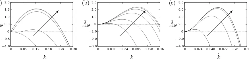
wavenumbers have been scaled in a manner that will be discussed below.) The general behaviour of the pertur-bation growth rates is similar, but there is one difference, illustrated in figure 4 a: forθ <1, as the Damk¨ohler num-bers become smaller the growth rates can become pos-itive for intermediate wavenumbers even in cases where
s remains negative for smaller wavenumbers. We will discuss this further below.
To obtain analytical results, we consider the asymp-totic limit in which both Damk¨ohler numbers become small, while their ratio remains of order unity. Accord-ingly, we writeDa1=δDˆ1andDa2=δDˆ2and consider
the limitδ→0 with ˆD1and ˆD2of order unity. Equation
(57) becomes
2ξ3+ 2δDˆ2Kξ2+ [
(K−1)(1−θ)k+ 2δDˆ1 ]
ξ
−δDˆ2K(1−K)k= 0. (70)
We first consider a na¨ıve expansion, in which all quan-tities other thanδare of order unity. Seeking an expan-sion of the formξ= Ω0+ Ω1δ+O(δ2), whereℜ(Ω0)>0,
we obtain the leading-order equation
2Ω30+ (K−1)(1−θ)kΩ0= 0, (71)
and thus
Ω20=(1−θ)(1−K)
2 k. (72)
Since 0< K <1, this is consistent if and only ifθ <1, and the corresponding asymptotic expansion fors=ξ2− k2 is
s= (1−θ)(1−K)
2 k−k
2
[image:9.595.326.559.389.448.2]+O(δ). (73)
Figure 4 a illustrates how well (73) captures the be-haviour ofs(k) as the Damk¨ohler numbers become small. Although, with the choice ofDa1/Da2 employed in this
figure, the system is always stable for small wavenum-bers, s(k) is positive for intermediate wavenumbersk≈
(1−θ)(1−K)/4 (which in this case givesk≈0.125). Whenθ≥1, the na¨ıve expansion is not consistent with the conditionℜ(ξ)>0, so we need to seek alternative ex-pansions in this regime. Motivated by the small-kresults (63) and (66), we define rescaled variables vias=δ2sˆand k=δkˆ, and thusξ=δξˆ, and we seek an expansion of the form ˆξ= ˆξ0+ ˆξ1δ+O(δ2). Substituting this expansion
into (70), we obtain
ˆ
ξ0=
ˆ
D2K(1−K)ˆk
(K−1)(1−θ)ˆk+ 2 ˆD1
. (74)
This expression for ˆξ0 remains finite for all ˆk as long as
(K−1)(1−θ)≥0, and so since 0< K <1 this expansion can be uniform in ˆk only if θ ≥1; it thus complements
the na¨ıve expansion described above. The corresponding expression for ˆsis
ˆ
s=
(
ˆ
D2K(1−K)
(K−1)(1−θ)ˆk+ 2 ˆD1 )2
−1
ˆk2+O(δ). (75)
Whenθ >1, equation (75) successfully captures the be-haviour ofs, as illustrated in figure 4 c. In particular, for small ˆk it predicts instability precisely when (65) holds, and as ˆk→ ∞the growth rate decays as ˆs∼ −kˆ2.
However, whenθ= 1, equation (75) fails to capture the decay terms which determine the position of the maxi-mum ofs, and it is necessary to seek a different rescaling ofξandk. Under any such scaling, the term in (70) pro-portional toξ2 is asymptotically smaller than the term
proportional toξ; on the other hand, to obtain a non-trivial dependence of ξ on k it is necessary to include all three remaining terms. This motivates the scaling
ξ = δ1/2ξ¯, s = δ¯s and k = δ1/2k¯, and the expansion ¯
ξ= ¯ξ0+ ¯ξ1δ1/2+O(δ) then leads to the depressed cubic
equation
¯
ξ30+ ˆD1ξ¯0−q= 0, where q=
ˆ
D2K(1−K)
2 ¯
k >0.
(76) The real root may be found explicitly by Cardano’s method, giving
¯
s=
√ q2
4 + ˆ
D3 1
27+
q
2
1/3
−
√ q2
4 + ˆ
D3 1
27−
q
2
1/3 2
−k¯2+O(δ1/2). (77)
Whenθ= 1, equation (77) successfully captures the be-haviour ofs, as illustrated in figure 4 b.
In summary, we find that in the limit in which both Damk¨ohler numbers become small while their ratio re-mains of order unity, the stability depends on the pa-rameter θ. For θ < 1, so that the surface tension de-pends principally on the surface concentration, instabili-ties occur at wavenumberskof order unity, corresponding to preferred wavelengths roughly an order of magnitude greater than the thicknessηof the surface layer, and can do so even when the system remains stable ask→0. In contrast, forθ≥1 the preferred wavenumberskdecrease along with the Damk¨ohler numbers; thus the long-wave stability criterion (65) continues to capture the behaviour of the system, and the preferred wavelength of instabili-ties becomes much larger than the thickness of the surface layer.
IV. SUMMARY AND CONCLUSIONS
(a)
0 0
.06 0.12 0.18 0.24 0.30
s ×102
k −1
.0
−0
.5
0 0
.5
1
.0
1
.5
2
.0 (b)
0 0
.032 0.064 0.096 0.128 0.16
¯ s ×103
¯ k −3
.0
−2
.0
−1
.0
0 1
.0
2
.0
3
.0 (c)
0 0
.024 0.048 0.072 0.96 0.12
ˆ s ×104
ˆ k −4
.0
−2
.0
0 2
.0
4
.0
6
.0
8
.0
FIG. 4. (a) Perturbation growth ratess(k) forK = 0.5 andθ = 0, withDa1/Da2 = 0.2 andDa2 = 1, 0.1, 0.01 and 0.001 (solid lines), together with the asymptotic result (73) (dashed lines). (b) Scaled perturbation growth rates ¯s(¯k) forK = 0.5 andθ= 1, withDa1/Da2= 0.1 andDa2= 1, 0.1, 0.01, 0.001 and 0.0001 (solid lines), together with the asymptotic result (77) (dashed lines). (c) Scaled perturbation growth rates ˆs(ˆk) forK= 0.5 andθ= 2, withDa1/Da2= 0.1 andDa2= 1, 0.1, 0.01 and 0.001 (solid lines), together with the asymptotic result (75) (dashed lines). The arrows show the direction of decreasing
Da2 in each case.
which naturally accommodates both classical surfac-tants and solutes with anti-surfactant properties. Un-der kinetic equilibrium between the free surface and the bulk, such models must agree with the surface-tension–concentration relationship described by the Gibbs isotherm (4) together with a suitable condition, such as the Henry isotherm, relating the equilibrium bulk and surface concentrations. When bulk–surface equilib-rium does not hold, there is, in principle, freedom to extend the model in various ways. However, care must then be taken to distinguish artefacts of the extension from genuine physical phenomena, and in the model pre-sented here we have included the parameterθ, which al-lows this point to be investigated.
Considering the stability of an infinitely deep, initially quiescent layer of fluid suggests that, in contrast to sur-factant solutions, anti-sursur-factant solutions may experi-ence an instability driven by the accumulation of solute in the surface at points of surface flow convergence. The preferred spatial scales of this instability are rather small, but are sufficiently large relative to the thickness of the surface layer that the model remains consistent. For fast bulk–surface kinetics, for which the Damk¨ohler numbers are of order unity, the parameterθis irrelevant to the sta-bility. For slower bulk–surface kinetics,θ plays a role in setting the spatial scale of the instability, and the version of the model for which surface tension depends solely on surface concentration (corresponding to θ = 0) predicts the shortest preferred wavelengths. This demonstrates that the precise formulation of the surface-tension law for anti-surfactants may have observable consequences, and deserves further investigation. It is possible, for ex-ample, that measurements using cantilever instruments could resolve the small-scale variations associated with the instability, while non-equilibrium surface-tension be-haviour may also become apparent in the development of foams [26].
The existence of a linear instability naturally raises the question of the state towards which the perturbed system evolves. Since this instability is essentially driven by
per-turbations to the concentration fields, we may speculate that the first variable to evolve beyond the linear regime will be either the surface or the bulk concentration. The instability could be restrained by the breakdown of the linear bulk–surface flux or through changes to the trans-port rates; ultimately, it could manifest itself through precipitation of the solute in regions where the perturbed concentration exceeds the saturation concentration of the solute. One experimentally observable signature of this instability, therefore, might be a tendency for solutes to precipitate from solution in the vicinity of a free surface, under conditions when the bulk concentration is some-what lower than its saturation value. An experimental investigation of this possibility would be of considerable interest.
Finally, we note that although the model presented here is consistent with the basic thermodynamics repre-sented by the Gibbs isotherm, it remains essentially an extension of the established modelling framework for sur-factants, and a gap still exists between fluid-dynamical models such as ours and more fundamental descriptions of salt solutions [12]. More sophisticated models, which take account of distinct species and their electrochem-ical interactions as well as appropriate non-equilibrium thermodynamics, may be required to bridge this gap.
ACKNOWLEDGMENTS
JJAC is supported by a University of Strathclyde Post-graduate Research Scholarship. SKW is supported by Leverhulme Trust Research Fellowship RF-2013-355.
Appendix A: The infinite-depth limit of the finite-depth stability problem
[image:10.595.91.529.55.162.2]fluid layer becomes infinite. We will demonstrate that the finite-depth problem is well posed for both surfac-tants and anti-surfacsurfac-tants, but that the only family of solutions available for surfactants becomes degenerate as the depth tends to infinity. A full investigation of finite-depth effects is ongoing.
For a layer of dimensionless depthd∗, the far-field con-ditions (28) are replaced by
u∗=0 and ∂c ∗
b
∂z∗ = 0 on z
∗=−d∗. (A1)
In turn, the far-field conditions (46) are replaced by the conditions
U(−d∗) = 0, W(−d∗) = 0, C′(−d∗) = 0, (A2) while the general solutions to (48) and (39) consistent
with these boundary conditions become
W(z∗) =
(
A1+A2 z∗ d∗
)
sinh(k(z∗+d∗)) −kd∗(A1−A2)
(
1 + z ∗
d∗ )
cosh(k(z∗+d∗)) (A3)
and
C(z) =A3cosh(ξ(z∗+d∗)), (A4)
where, as before, we have written ξ = √k2+s. Note
that we require thatξ̸= 0, i.e.s̸=−k2, but impose no further condition onξ. Henceforth we drop the star on
d∗ for brevity.
The solvability condition becomes
kdc(kd)−s(kd) −kdc(kd) 0 0
2k2dc(kd) −2(1 +k 2d2)
d c(kd)−2ks(kd) kθ(1−K) c(ξd)
k(θ−1)(K−1)
K
0 0 ξs(ξd)+Da2Kc(ξd) −Da2
Kk2ds(kd) −K(1 +k
2d2)
d s(kd)−Kkc(kd) −Da1Kc(ξd) ξ
2+Da 1
= 0, (A5)
where we have written s and c as shorthand for sinh and cosh respectively.
Solving (A5) numerically in the parameter regime (33), we typically find that if 0 < K < 1 then instability is possible for a range of small values ofk, as in the infinite-depth problem, whereas if K > 1 then no instability occurs. A detailed discussion of the results for finite d
lies beyond the scope of this appendix; instead, here we will seek asymptotic results asd→ ∞. The form of the exponential terms in (A5) makes it natural to consider four distinguished limits, depending on the combination of k, kd, ξ and ξd that is taken to remain finite and non-zero in this limit; we consider them in turn.
Case (i): ℜ(ξ) and k remain finite and non-zero as d → ∞. This is the case implicitly considered in §III by postulating an infinitely deep body of fluid. In this limit we may approximate all of the hyperbolic terms in (A5) by exponentials. We must consider the cases ℜ(ξ)≷0 separately in order to discard the correct ex-ponential terms; combining the results we find that the solvability condition (A5) reduces to
2ξ3sgn(ξ)+2Da2Kξ2+[(K−1)(1−θ)k+2Da1] sgn(ξ)ξ
+Da2Kk(K−1) +O (
e−2kd,e−2sgn(ξ)ξd
)
= 0, (A6)
where sgn(ξ) =±1 ifℜ(ξ)≷0.
If ℜ(ξ) > 0 then, as we have seen in §III C 1, only the regime 0 < K < 1 permits consistent solutions for
long waves. Alternatively, ifℜ(ξ)< 0 then by defining
ξ′=−ξwe again find that there are consistent solutions for long waves only when 0< K <1. We conclude that whenK >1, in order to find consistent solutions across allk we must consider a different distinguished limit.
Case (ii): ℜ(ξ) andkd remain finite and non-zero as d→ ∞. We now consider the possibility thatξremains of order unity (maintaining the possibility thats=O(1)) asd→ ∞, but that this occurs only for very long waves. We thus define κ = kd and set κ = O(1) as d → ∞. Again considering ℜ(ξ) ≷ 0 separately, we reduce the solvability condition (A5) to
(
ξ3+ξ2sgn(ξ)Da2K+Da1ξ )
(cosh(κ) sinh(κ)−κ)
+O
(
1
d,e
−2sgn(ξ)ξd )
= 0. (A7)
Since ξ̸= 0 by assumption and the factor cosh(κ) sinh(κ) − κ is strictly positive for κ >0, we conclude thatξ must satisfy the quadratic equation
ξ2 + ξsgn(ξ)Da
2K + Da1 = 0. Again considering
separately the cases sgn(ξ) =±1, we conclude that there are no consistent solutions in this distinguished limit for any positive value ofK.
we reduce the solvability condition (A5) to
[
kd2(K−1)(1−θ) + 2Da1d2+ 2Ξ2 ]
Ξ sinh(Ξ) +Da2Kd
[
(K−1)d2k+ 2Ξ2]cosh(Ξ)+O(e−2kd)= 0.
(A8)
As d→ ∞, the dominant terms are those ind3, and so
the solvability condition reduces to cosh(Ξ) = 0, with solutions Ξ =(n+12)πi forn∈Z. The solutions yield
s∼ −k2− (
n+1
2
)2 π2
d2, (A9)
which describe stable modes, independent of K and de-caying a little faster than the rate s = −k2 set by the
diffusion of a vertically constant perturbation. Crucially, when we take the limit of infinite depth, these modes col-lapse ontos=−k2. The loss of these modes represents
a degeneracy in the problem, which is important only if no other modes exist.
Case (iv): ξd and kd remain finite and non-zero as d→ ∞. In this final case, we set Ξ =ξdandκ=kdas before, and the solvability condition (A5) reduces to
Da2K(K−1)κ (
sinh2(κ)−κ2)cosh(Ξ)
+ 2Da1(cosh(κ) sinh(κ)−κ) Ξ sinh(Ξ) +O (
1
d )
= 0.
(A10)
Rearranging then yields
Ξ tanh(Ξ)∼ Da2K(1−K) 2Da1
κ(sinh2(κ)−κ2)
(cosh(κ) sinh(κ)−κ). (A11)
The function ofκon the right-hand side is strictly posi-tive forκ >0, so the sign of the right-hand side is identi-cal to the sign of the factor 1−K. Hence, it can be shown that for 0< K <1 we obtain modes with Ξ∈ R+ and thuss >−k2; these modes persist asd→ ∞, although
they occur at wavelengths that scale with d, while the growth rates scale with 1/d2. ForK > 1, we must seek imaginary solutions for Ξ. We may write Ξ = iχso that the left-hand side becomes−χtan(χ), and so we obtain a spectrum of modes withs∼ −κ2/d2−χ2/d2<−k2.
The overall conclusion from this asymptotic analysis is that although the finite-depth stability problem is well posed for both surfactants and anti-surfactants, the limit
d→ ∞is degenerate. Only a particular family of modes survives in this limit, and this family is available only for anti-surfactants, 0 < K < 1, for which it provides the dominant mode.
The modes that degenerate in the limit d → ∞ do so because their spatial scale is naturally set by the depth of the layer, and becomes ill-defined in this limit. In contrast, the bulk concentration field for the non-degenerating modes has a boundary-layer structure and the depth of the layer becomes irrelevant. Since, from (39), the thickness of any concentration boundary layer must scale as ξ = √k2+s, boundary layers can occur
only whenℜ(s)>−k2, i.e. when the concentration per-turbation is not decaying as rapidly as it would by dif-fusion alone. To resist this diffusive decay an instability mechanism must act near or at the surface, and thus perturbations with this structure are available only for anti-surfactants.
[1] D. J. Shaw,Introduction to Colloid and Surface Chem-istry, 2nd ed. (Butterworths, 1970)
[2] A. P. dos Santos, A. Diehl, and Y. Levin, Langmuir26, 10778 (2010)
[3] G. V´azquez, E. Alvarez, and J. M. Navaza, Journal of Chemical & Engineering Data40, 611 (1995)
[4] M. S. Borgas and J. B. Grotberg, Journal of Fluid Me-chanics 193, 151 (1988)
[5] O. E. Jensen and J. B. Grotberg, Physics of Fluids A5, 58 (1993)
[6] O. K. Matar and S. M. Troian, Physics of Fluids11, 3232 (1999)
[7] G. Karapetsas, R. V. Craster, and O. K. Matar, Journal of Fluid Mechanics670, 5 (2011)
[8] G. Karapetsas and V. Bontozoglou, Journal of Fluid Me-chanics 741, 139 (2014)
[9] C.-H. Chang and E. I. Franses, Colloids and Surfaces A 100, 1 (1995)
[10] C. J. W. Breward, R. C. Darton, P. D. Howell, and J. R. Ockendon, Chemical Engineering Science56, 2867 (2001) [11] C. E. Morgan, C. J. W. Breward, I. M. Griffiths, P. D.
Howell, J. Penfold, R. K. Thomas, I. Tucker, J. T. Petkov, and J. R. P. Webster, Langmuir28, 17339 (2012) [12] P. B. Petersen and R. J. Saykally, Annual Review of
Physical Chemistry57, 333 (2006)
[13] T. Markovich, D. Andelman, and R. Podgornik, Euro-physics Letters106, 16002 (2014)
[14] More precisely, the Gibbs isotherm relates σeq to the chemical potentialµdefined by dµ=RTd(loga), where
a is the thermodynamic activity, but for sufficiently di-lute solutions a is close to cb, and hence equation (4) holds.
[15] The conditions 1−K ≶ 0 may be written as KH ≷ 0, whereKH=−η(1−K). For surfactants,KH>0 is the equilibrium adsorption constant [9].
[16] A. Pereira and S. Kalliadasis, The European Physical Journal Applied Physics44, 211 (2008)
[17] H. A. Stone, Physics of Fluids A2, 111 (1990)
[18] H. Wong, D. Rumschitzki, and C. Maldarelli, Physics of Fluids8, 3203 (1996)
[20] I. Hashim and S. K. Wilson, Zeitschrift f¨ur angewandte Mathematik und Physik50, 546 (1999)
[21] W. M. Haynes, ed., CRC Handbook of Chemistry and Physics, 94th ed. (CRC Press, Boca Raton, FL, 2013) [22] S. Z. Mikhail and W. R. Kimel, Journal of Chemical &
Engineering Data4, 533 (1961)
[23] K. R. Harris and P. J. Newitt, Journal of Physical Chem-istry A103, 6508 (1999)
[24] B. A. Noskov, Advances in Colloid and Interface Science 69, 63 (1996)
[25] S. E. Orchard, Journal of Applied Sciences Research11, 451 (1962)