Parameter Reduction in Log-normal Chain-ladder Models

City, University of London Institutional Repository

Citation

:

Verrall, R. J. & Wüthrich, M. V. (2015). Parameter Reduction in Log-normal Chain-ladder Models. European Actuarial Journal, 5(2), pp. 355-380. doi: 10.1007/s13385-015-0114-7

This is the accepted version of the paper.

This version of the publication may differ from the final published

version.

Permanent repository link:

http://openaccess.city.ac.uk/12436/

Link to published version

:

http://dx.doi.org/10.1007/s13385-015-0114-7

Copyright and reuse:

City Research Online aims to make research

outputs of City, University of London available to a wider audience.

Copyright and Moral Rights remain with the author(s) and/or copyright

holders. URLs from City Research Online may be freely distributed and

linked to.

City Research Online: http://openaccess.city.ac.uk/ [email protected]

Parameter Reduction in Log-Normal Chain-Ladder Models

--Manuscript

Draft--Manuscript Number: EUAJ-D-13-00036R2

Full Title: Parameter Reduction in Log-Normal Chain-Ladder Models Article Type: Original Research Paper

Keywords: claims reserving; loss reserving; CL method; CL factors; non-life insurance; risk; general insurance; parameter reduction; tail factor

Corresponding Author: Richard Verrall UNITED KINGDOM Corresponding Author Secondary

Information:

Corresponding Author's Institution: Corresponding Author's Secondary Institution:

First Author: Richard Verrall First Author Secondary Information:

Order of Authors: Richard Verrall Mario Wüthrich Order of Authors Secondary Information:

Funding Information:

Abstract: Multiplicative chain-ladder (CL) models are characterized by CL factors that explain the development of claims from one period to the next. In classical CL models every development period has its own CL factor. In the present paper we give a method describing how some of these CL factors can be modeled by a joint functional dependence. This joint functional form reduces the number of model parameters needed.

Parameter Reduction in Log-Normal Chain-Ladder Models

Richard J. Verrall∗ Mario V. W¨uthrich†‡

July 24, 2015

Abstract

Multiplicative chain-ladder (CL) models are characterized by CL factors that explain the development of claims from one period to the next. In classical CL models every development period has its own CL factor. In the present paper we give a method describing how some of these CL factors can be modeled by a joint functional dependence. This joint functional form reduces the number of model parameters needed.

∗

Cass Business School, City University London, 106 Bunhill Row, London EC1Y 8T2, UK

†

ETH Zurich, RiskLab Switzerland, Department of Mathematics, 8092 Zurich, Switzerland

Parameter Reduction in Log-Normal Chain-Ladder Models

July 24, 2015

Abstract

Multiplicative chain-ladder (CL) models are characterized by CL factors that explain the

development of claims from one period to the next. In classical CL models every development period has its own CL factor. In the present paper we give a method describing how some

of these CL factors can be modeled by a joint functional dependence. This joint functional form reduces the number of model parameters needed.

1

Introduction

Verrall-W¨uthrich [14] considered the practical issue of parameter reduction with applications to claims reserving models. The issue of over-parametrization is often raised in relation to the chain-ladder (CL) technique because there is an extra parameter (CL factor) for each development period. This also means that it is not possible to extrapolate individual CL factors to create “tail factors” without making further assumptions. In this paper and in Verrall-W¨uthrich [14] we tackle this problem by formulating what is often done practically in an ad hoc manner into a statistical method of model selection. The drawback of Verrall-W¨uthrich [14] was that it was necessary to solve the problem using numerical methods since closed-form solutions do not exist for the general case. For this reason, reversible jump Markov chain Monte Carlo (RJMCMC) methods were used. These methods are not straightforward to implement and they can be unstable and time-consuming. In this paper, we restrict attention to the log-normal distribution with conjugate priors. This leads to elegant analytical results that allow to do model selection in a direct manner.

An important feature of the approach, both in this paper and in Verrall-W¨uthrich [14], is that a functional dependence allows for extrapolation of the claims development beyond the latest observed delay period in the data, and for creation of tail factors in a very natural way. Thus, these two papers show how the important issue of parameter reduction in claims reserving can be addressed. The choice is between the more general distributional assumptions and more complex implementation in Verrall-W¨uthrich [14] or the more restricted log-normal case here with closed form solutions.

The paper is set out as follows: in the next section we define the Bayesian log-normal CL model and we provide first properties. In Section 3 we discuss parameter estimation, followed by Section 4 where we describe model selection techniques. In Section 5 we explain claims

prediction, uncertainty analysis and extrapolation for tail factor estimation. Finally, in Section 6 we revisit the liability example of Verrall-W¨uthrich [14].

2

Bayesian log-normal CL model with conjugate priors

2.1 Model assumptions

To study the problem of parameter reduction in CL models we embed Hertig’s [7] log-normal CL model into a Bayesian modeling framework. Based on this Bayesian approach we aim to determine the set of CL factors that can be explained by a common functional dependence. For this purpose we introduce atruncation indexk∈ {1, . . . , J−1}. Before the truncation index each CL factor is characterized by an individual development parameter and beyond the truncation index all CL factors are described by a functional dependence of common parameters. This way we obtain awhole familyof modelsM(k)_{,k∈ {1, . . . , J−1}, each modelM}(k) _{having a different} number of model parameters. Model selection will then be done on this family of models. The models are set out formally in Model Assumptions 2.1, below.

We introduce the following notation, for detailed background information on claims reserving we refer to Chapter 9 in W¨uthrich [16]. We denote accident years byi∈ {1, . . . , I}and development years by j ∈ {0, . . . , J}. I is the last accident year considered and J is the maximal possible development delay. Throughout we assumeI > J. The cumulative claim of accident yeariafter development year j is denoted by Ci,j, andCi,J is called ultimate claim or total claim amount

of accident yeari. At time I we have observations

D_I ={Ci,j; i+j≤I, 1≤i≤I, 0≤j≤J},

and our aim is to predict the inexperienced part of the claims given by

D_Ic={Ci,j; i+j > I, 1≤i≤I, 0≤j≤J}.

In order to achieve this task we make the following model assumptions for the claims (Ci,j)i,j.

Model Assumptions 2.1 (Bayesian log-normal CL models) Choose a fixed truncation

index k ∈ {1, . . . , J −1}. Model M(k) _{is given by the following assumptions. There are given}

standard deviation parameters σ= (σ0, . . . , σJ)0 ∈RJ++1.

• Given parameter θ = (θ0, . . . , θJ)0, the sequences (Ci,j)j=0,...,J are independent (in i)

Markov processes (in j) with log-link ratios

ξi,j = log

Ci,j

Ci,j−1

−1

{θ,Ci,j−1}

∼ N(θj, σj2) for j= 0, . . . , J,

where we set Ci,−1 =νi for i∈ {1, . . . , I} with given constants νi >0.

• Assume that the parameter Θ(k)= (θ0, . . . , θk−1, α, β)0 has a multivariate Gaussian

distri-bution

Θ(k) = (θ0, . . . , θk−1, α, β)0 ∼ N

µ(k), T(k), 3

with given prior mean µ(k) = (µ0, . . . , µk−1, µα, µβ)0 ∈ Rk+2 and positive definite prior

covariance matrix T(k) = diag(τ₀2, . . . , τ_k2₋₁, τ_α2, τ_β2)∈_R(k+2)×(k+2)_{. For j ∈ {k, . . . , J} we}

set

θj =α−jβ.

2

The interpretation of Model Assumptions 2.1 will be divided into three parts, see Remarks 2.2, 2.4 and 2.6 below.

Remarks 2.2 (to Model Assumptions 2.1, part 1/3)

• Cumulative claims satisfy the multiplicative structure

Ci,j =Ci,j−1(exp{ξi,j}+ 1). (2.1)

Thus, we have a multiplicative CL structure described by a shifted log-normal distribution, and the excess claim Ci,j −Ci,j−1 has a multiplicative random structure described by a log-normal distribution. This structure is in particular appealing for inflation modeling on payments, see Shi et al. [12] and W¨uthrich [15].

Property (2.1) might be criticized because it requires non-negative excess claims. If this is an undesired model property one could also study the model Ci,j = Ci,j−1exp{ξi,j}.

The mathematical techniques would be exactly the same because we will only work on the log-link ratiosξi,j, see Lemma 2.5 below, however the modeling of the tail behavior would

become more sophisticated. Therefore, we refrain from considering the latter model in this work.

• For fixed truncation indexkparameter θ in model M(k) _{takes the following form}

θ = (θ0, . . . , θk−1, α−kβ, . . . , α−J β)0. (2.2) The first k components of θ are modeled by individual parameters θj for j < k and the

remaining components are characterized by the two common parameters α and β and a linear functional dependence, that is,θj+1=θj−β forj≥k. The aim will be to find the

optimal truncation indexkand the optimal modelM(k)_{, respectively, for a given data set}

D_I.

• The distribution Θ(k) ∼ N µ(k), T(k) reflects the prior knowledge about parameters. This can come from expert opinion, from market information or from a regulatory view-point. If there is only little information available or if we have heterogeneous beliefs we choose a covariance matrix T(k) with big variances, which reflects heterogeneity and/or uncertainty.

• Note that we have assumed prior independence T(k) = diag(τ₀2, . . . , τ_k2₋₁, τ_α2, τ_β2) between the components of parameter Θ(k). In view of the following derivations this seems to be

an unnecessary restriction because the whole theory holds true for any positive definite covariance matrixT(k). We do this choice to more clearly separate the effects coming from different model characteristics. In practical applications this choice should be revised since dependence in T(k) may also help to incorporate shape constraints in tail factors.

• If there are known differences νi > 0 between the accident years i ∈ {1, . . . , I} we can

implement these differences by initializing Ci,−1 = νi. If there is no prior information

available about these differences we set νi = 1 for all i. These choices will not influence

the prediction of Dc

I, given the observations DI and the parameters Θ(k), under our

inde-pendence assumptions, becauseCi,0 ∈ DI for alli≤I. This is demonstrated in the next

corollary. However, these differences will become important if we choose more general correlation structures in T(k) and between the components of (ξi,j)i,j, see (2.5) below, for

the latter we also refer to Shi et al. [12] and W¨uthrich [15].

An easy consequence of the model assumptions is the following corollary (the proof is completely similar to the one of Lemma 5.2 in W¨uthrich-Merz [17]).

Corollary 2.3 Choose model M(k)_{. Under Model Assumptions 2.1 we have for i > I−J}

E h

Ci,J DI,Θ

(k)i _{= C}

i,I−i J Y

j=I−i+1 exp

θj+σj2/2 + 1

= Ci,I−i k−1

Y

j=I−i+1

expθj +σj2/2 + 1

J Y

j=(I−i+1)∨k

expα−jβ+σ_j2/2 + 1,

where x∨y= max{x, y} and an empty product is defined to be equal to 1.

Remarks 2.4 (to Model Assumptions 2.1, part 2/3)

• Corollary 2.3 provides the multiplicative CL structure for given parametersΘ(k)in model

M(k) _{with CL factors defined by f}

j = (exp{θj+σ2j/2}+ 1). It also shows that the choice

of νi has no influence on the prediction under our independence assumptions.

• Before the truncation indexk every CL factor is modeled individually byθj, j < k, after

the truncation index kthe CL factors are modeled by the two common parametersα and

β using an exponential decay with rate β forj≥k, that is,

fj = exp

α−jβ+σ_j2/2 + 1,

see also (2.2). Thus, we use a curve fitting method by specifying an exponentially decaying function. From a purely theoretical point of view the fitted curve could have any other functional form and our theory would still work. Choice (2.2) has the advantage of simplic-ity and tractabilsimplic-ity whereas many other functional forms will in general require simulation based solutions similar to Verrall-W¨uthrich [14]. The interested reader is referred to De Jong-Zehnwirth [4], Section 4 in England-Verrall [5], Verrall [13] and, in particular, Section 5 of Boor [2] for other functional forms. In our numerical example, the exponential decay seems quite reasonable, see Figure 5 below, an other possible choice is provided in (6.3) below.

2.2 Properties of Bayesian log-normal CL models

We introduce some notation that simplifies the outline. The cardinality of the set of indexes

I ={1, . . . , I} × {0, . . . , J}is denoted byd=I(J+ 1) and we define the vector of log-link ratios

ξ= (ξi,j)0i=1,...,I;j=0,...,J = (ξ1,0, . . . , ξ1,J, . . . , ξI,0, . . . , ξI,J)0 ∈Rd.

The joint density in modelM(k) _{ofξ and parametersΘ}(k) _{at position (ξ,θ}(k)_{) is given by}

f(k)

ξ,θ(k)

=f(k)

ξ

θ

(k) _p(k)_θ(k)_{, (2.3)}

where we have prior density

p(k)

θ(k)

= 1

(2π)k/2+1 _det(T(k)₎1/2 exp

−1

2 (θ

(k)_−µ(k)₎0

(T(k))−1 (θ(k)−µ(k))

,

and likelihood function of the log-link ratiosξ, given parameters θ(k),

f(k)ξ

θ

(k)₌ 1

(2π)d/2 _det(Σ)1/2 exp

−1

2 (ξ−A

(k)_θ(k)₎0 _Σ−1 _(ξ−A(k)_θ(k)₎

, (2.4)

where we denote the diagonal covariance matrix of the log-link ratios by

Σ = diag(σ2₀, . . . , σ_J2, . . . , σ2₀, . . . , σ_J2)∈Rd×d, (2.5)

and we define the matrix A(k) = (B_k0, . . . , B_k0)0 ∈Rd×(k+2) such that matrix Bk ∈R(J+1)×(k+2)

describes the parameters for a single accident yeari and is given by

B_k0 =



     

0 . . . 0

1 ... ...

0 . . . 0 0 · · · 0 1 . . . 1 0 · · · 0 −k . . . −J



      ,

with1∈_Rk×k _{being the identity matrix. This choice implies, see also (2.2),}

θ=BkΘ(k)∈RJ+1 and E h

ξ

Θ

(k)i_=A(k)_Θ(k) _∈

Rd.

From this we see that A(k) allows the conditional expectation of the log-link ratios ξ to be expressed in terms of the parameters Θ(k) in model M(k)_{. An easy consequence of Model} Assumptions 2.1 is the following lemma (we leave the proof to the reader).

Lemma 2.5 Set Model Assumptions 2.1 for model M(k)_{. The joint density f}(k)_(ξ,θ(k)_{) of ξ}

and Θ(k) describes a multivariate Gaussian distribution with

ξ

Θ(k) !

∼ N

A(k)µ(k) µ(k)

!

, Σ +A

(k)_T(k)_(A(k)₎0 _A(k)_T(k)

T(k)(A(k))0 T(k) !!

.

The random vectorξ has in modelM(k) _{a multivariate Gaussian distribution with meanm}(k) ₌

A(k)µ(k) and covariance matrix Σ(k) = Σ +A(k)T(k)(A(k))0. 3

Remarks 2.6 (to Model Assumptions 2.1, part 3/3)

• We have assumed that all log-link ratios ξi,j are conditionally independent. This

inde-pendence assumption could be replaced by any multivariate Gaussian distribution and we would still get closed form solutions, see Merz et al. [11], Shi et al. [12] and W¨uthrich [15]. At the current stage we refrain from doing so because we do not want to mix dependence with tail factor estimation, but it is worth analyzing this extension numerically in future work. Basically, it means that the covariance matrix Σ, defined in (2.5), needs to be re-placed by any symmetric positive definite matrix and then the whole theory, as presented in this article, still runs through.

• One might criticize the Gaussian distribution assumption of the log-link ratios ξi,j and

the corresponding Gaussian priorsΘ(k). Our model belongs to the Bayesian models with conjugate priors which have the advantage of staying in the same family of distributions for the posteriors, see Section 2.5 in B¨uhlmann-Gisler [3] and Section 8.1 in W¨uthrich [16]. Thanks to the multivariate Gaussian assumptions we obtain closed form solutions as seen in Lemma 2.5 and Corollaries 3.1 and 3.2. Other distributional assumptions, in general, only allow for simulation results, similar to Verrall-W¨uthrich [14], where (complicated) re-versible jump Markov chain Monte Carlo (RJMCMC) simulations are used. The purpose of this paper is to present a model which has a closed form solution, this facilitates sensi-tivity analysis. The explicit choice of the distributional assumption will become especially important for the calculation of tail-sensitive risk measures such as Tail-Value-at-Risk. Our risk measure choice (5.1) is less tail-sensitive and, therefore, the log-normal model is usually sufficient.

• If we relax the distributional assumptions we may consider distributions from the expo-nential dispersion family with conjugate priors, see Lee-Nelder [9, 10], Gigante et al. [6], Section 2.5 in B¨uhlmann-Gisler [3] and Section 8.1 in W¨uthrich [16]. In our situation this would provide the following distributional form

logf_HGLM(k)

ξ,θ(k)

=

J X

j=0

I X

i=1

wi,j

φ [ξi,jθj −b(θj)] + logc(ξi,j, wi,j/φ) (2.6)

+

k−1

X

j=0 1

ψj

[µjθj−b(θj)] + X

a∈{α,β}

1

ψa

[µaa−b(a)] + const.

The first term describes the log-likelihood function of the log-link ratios ξ, given the parameters θ =Bkθ(k). The second term describes the parameters θ(k) that model the

firstkof the CL factors individually and the remaining CL factors are modeled by common parametersαandβ(using the linear functional dependence). Our Gaussian model uses the generic choice b(θ) =θ2/2. The general form (2.6) is less tractable than the Gaussian one because marginals do not have explicit forms. Formula (2.6) is very close to hierarchical generalized likelihood models (HGLMs) and calibration can also be done using maximum

likelihood estimation (MLE) methods, see Gigante et al. [6]. Since this framework is less tractable, we have decided to stay within Assumptions 2.1 for the present work.

3

Model calibration in a fixed model

M

(k)

We fix a truncation indexk and a model M(k) _{and assume that we have observationsD}

I with

I > J. There are the parameters Σ = diag(σ₀2, . . . , σ2_J, . . . , σ₀2, . . . , σ_J2), µ(k) and T(k) that need to be specified. As explained in Remarks 2.2, the parameters µ(k) and T(k) correspond to prior knowledge or a market view and, therefore, cannot be calibrated from individual dataD_I. Thus, we either have this prior knowledge and thenµ(k) andT(k)describe this information or there is no prior knowledge in which case we choose large variances forT(k)which make the influence of the prior distribution negligible (non-informative) for the prediction of Dc

I.

There remains the calibration of Σ. This is described in Subsection 3.1 below. In view of the HGLM approach (2.6) we could also get to a slightly different model interpretation (more in the light of a frequentist’s approach). This leads to another way of model calibration which we would briefly like to present in Subsection 3.2.

3.1 Model calibration using an empirical Bayesian approach

By an abuse of notation we set (note that the correspondingσ-fields generated byCi,j andξi,j,

i+j≤I, are the same)

DI ={ξi,j; i+j≤I, 1≤i≤I, 0≤j≤J}.

Let c =|DI|< d denote the cardinality of DI. Then, we define the projections P1 :Rd → Rc

and P2 :Rd→Rd−c such that we obtain a bijective decomposition

ξ 7→ ξDI,ξDIc

= (P1ξ, P2ξ),

with ξDI = P1ξ containing exactly the components of ξ which are in DI, i.e. are observed at

timeI, andξDc

I =P2ξ are the remaining components ofξ. A direct consequence of Lemma 2.5

is that the parameters θ(k) can be integrated out in the following sense.

Corollary 3.1 (marginal likelihood functions) Set Model Assumptions 2.1 for modelM(k)_.

The random vector (ξDI,ξDIc) has a multivariate Gaussian distribution with the first two mo-ments given by

µ(_Ik)=EξDI

=P1A(k)µ(k) and Σ(_Ik)= Cov ξDI

=P1Σ(k)P10,

µ(_Ikc)=E h

ξDc I i

=P2A(k)µ(k) and Σ(_Ikc)= Cov

ξDc I

=P2Σ(k)P20.

The covariance matrix between the components ξ_D

I and ξDcI is given by

(Σ(_Ikc)_,I)0 = Σ

(k)

I,Ic = Cov

ξ_DI,ξ_Dc I

=P1Σ(k)P20.

This corollary is an easy consequence of Lemma 2.5 because it only describes a permutation (relabeling) of the components of ξ. However, it is useful for parameter calibration, prediction and model selection as we will see below.

Corollary 3.2 (predictive distribution) Set Model Assumptions 2.1 for model M(k)_{. The}

conditional distribution of ξ_Dc

I, given ξDI, is a multivariate Gaussian distribution with condi-tional mean given by

µpost(_Ic k) =E h

ξDc I ξDI

i

=µ(_Ikc)+ Σ

(k)

Ic_,I

Σ(_Ik)

−1

ξDI −µ

(k)

I

,

and conditional covariance matrix given by

Σpost(_Ic k)= Cov

ξDc I ξDI

= Σ(_Ikc)−Σ

(k)

Ic_,I

Σ(_Ik)

−1

Σ(_I,Ik)c.

Proof of Corollary 3.2. The proof is a standard consequence of Corollary 3.1, see for instance Result 4.6 in

Johnson-Wichern [8]. 2

In view of Corollary 3.2 we only need to calibrate the standard deviation parameters σ which enter Σ and Σ(k), respectively, and then we can predict the lower triangle in model M(k)_{. In a} full Bayesian approach we choose a prior distribution for these standard deviation parameters. However, then we lose analytical tractability. Therefore, we turn here to an empirical Bayesian viewpoint, estimating these parameters with MLE methods. The marginal likelihood function of the observationsξDI for the standard deviation parameters σ is given by, see Corollary 3.1,

L(k) σ|ξDI

= f(k)(ξDI) (3.1)

= 1

(2π)c/2 _det(Σ(k)

I )1/2

exp

−1

2(ξDI −µ

(k)

I )

0

(Σ(_Ik))−1(ξDI −µ

(k)

I )

.

Maximization of this marginal likelihood function provides the MLEσ_b(k)forσin modelM(k)_{. If} we replace the standard deviation parametersσ by their MLEsσb

(k)

then Corollary 3.2 provides the full predictive distribution of the lower triangle Dc

I ={ξi,j; i+j > I}, conditionally given

the observations D_I, that is,

b

ξ(_Dkc) I _{D

I}

∼ N µ_bpost(_Ic k),Σb

post(k)

Ic

, (3.2)

whereµb

post(k)

Ic andΣb

post(k)

Ic correspond toµ

post(k)

Ic and Σ

post(k)

Ic withσ(k) replaced byσ_b(k).

3.2 Hierarchical maximum likelihood estimation

The model calibration in the previous section was done using the interpretation of having a Bayesian model. However, we could also interpret this model as a HGLM, see Lee-Nelder [9, 10] and Gigante et al. [6]. We explain this in more detail next. For HGLM we assume a hierarchical model in the sense that there is a first level of effects

θ(k)∼ N(µ(k), T(k)). 3

This may reflect the regulatory viewpoint whereµ(k) describes the insurance market in average andθ(k)the company specific features. Based on this first level, we then have responsesξ|_{θ(k)_} ∼ f(k)(ξ|θ(k)) according to (2.4). These use the linear predictor given by A(k)θ(k). Lee-Nelder [9] introduced theh-likelihood of the dataD_I and the effects θ(k) given by, see also formula (8) in Gigante et al. [6],

h(k)

ξDI,θ

(k) _∝

k−1

X

j=0

"_I−j X

i=1

− 1

2σ2

j

(ξi,j−θj)2−logσj !

− 1

2τ2

j

(θj −µj)2 #

(3.3)

+

J X

j=k I−j X

i=1

− 1

2σ_j2 (ξi,j−(α−jβ))

2_−logσ

j !

+ X

a∈{α,β}

− 1

2τ2

a

(a−µa)2,

where all remaining normalizing constants are put into the proportionality sign∝. For conjugate HGLMs, the h-likelihood (3.3) can be viewed as anaugmented GLM with data D_I and pseudo-data µ(k). Therefore, for given T(k), the effectsθ(k) and the standard deviation parametersσ

can be estimated by MLE providing the following system equations

∂h(k)ξDI,θ

(k)

∂θj

= 0 and

∂h(k)ξDI,θ

(k)

∂σj

= 0 forj= 0, . . . , k−1, (3.4)

∂h(k)

ξDI,θ

(k)

∂(α, β) =0 and

∂h(k)

ξDI,θ

(k)

∂σj

= 0 forj=k, . . . , J . (3.5)

The solution of (3.4)-(3.5) provides the MLEs b b

θ

(k) and σb_b

(k)

in model M(k)_{. Observe that for}

j≤k−1 we can do an optimization for each development year individually, whereas forj ≥k

we do an optimization over all development years simultaneously.

If there is no market view about µ(k), we set τ1=. . .=τk−1 =τα =τβ =∞ on the right-hand

side of (3.3). Then the (non-existent) market knowledgeµ(k) _{disappears and we are back in the} classical GLM context, optimizing the right-hand side of (3.3) neglecting the terms containing any additional knowledge (no augmentation).

The random variablesξi,j ∈ Dc_I in the lower triangle are then approximated by independent (for

i+j > I) log-link ratios

b b ξ

(k)

i,j _{D

I} ∼ N

b b θ

(k)

j ,σb_b

(k)

j

. (3.6)

Note that this second estimation approach also works in the more general HGLM situation given in (2.6). The disadvantage of (3.6) is that it only considers the point estimator b

b

θ

(k) and then simulates conditionally on this estimator according to (3.6). But unlike (3.2), it does not consider uncertainty in this estimator and the quantification of this uncertainty is only obtained by rather involved approximations, using asymptotic MLE results (see for instance Section 6.4.3 in W¨uthrich-Merz [17] and Gigante et al. [6]) or bootstrap simulations. Therefore, we prefer the empirical Bayesian approach of Subsection 3.1.

4

Model selection and parameter reduction

In the previous sections we have defined a whole family of modelsM(k)_{,k∈ {1, . . . , J−1}. We} now try to find the model that fits the data ξDI best.

4.1 Model selection: Bayesian approach

The marginal distribution (3.1) has a very appealing form that allows for model selection. The general difficulty in such model selection problems is that the dimension of the parameter space may be different in each model M(k)_{. Therefore, a simulation approach for model selection} needs a sophisticated design because these simulations need to experience parameter spaces having (potentially) different dimensions. To overcome this problem state-of-the-art simulation uses RJMCMC methods as demonstrated in Verrall-W¨uthrich [14]. The general design of this RJMCMC simulation is very involved. The beauty of our model lies in the fact that we can completely avoid simulations because (3.1) has a sufficiently nice closed form. This we explain next.

We choose a prior distribution on the modelsM(k)_{,k∈ {1, . . . , J−1}, themselves, i.e.}

p

M(k)>0 with

J−1

X

k=1

p

M(k)= 1.

The posterior distribution on the model space, given observationξDI, is given by p

M(k)

ξDI

= f (k)_(ξ

DI) p M

(k) PJ−1

l=1 f(l)(ξDI) p M

(l) ∝ f

(k)_(ξ

DI) p

M(k), (4.1)

where the marginal f(k)(ξDI) is explicitly given in (3.1). Thus, model selection tells that we

should choose the model with the maximal posterior probability weight p(M(k)_|ξ

DI) in (4.1).

If there is no dominant model we may also choose model averaging using these posterior model probabilities. Averaging then also includes a component for model uncertainty within this family of models M(k)_{,k∈ {1, . . . , J −1}.}

The latter may also raise the question whether we should speak about different models M(k)_,

k∈ {1, . . . , J −1}, or whether we have simply an overall Bayesian model. Following RJMCMC methods we prefer the first terminology because it emphasizes that parameter spaces may have different dimensions which need to be experienced. This always needs a rather careful treatment, in particular, if simulation methods are applied.

4.2 Model selection: HGLM approach

In the previous subsection, we have done model selection in a Bayesian approach. If we use the HGLM model interpretation of Section 3.2, we could also use other statistical measures for model selection. In order to find the parameters in the HGLM approach we consider the

h-likelihood h(k) in each modelM(k)_{, see (3.3). That is, in model M}(k)_{, k= 1, . . . , J −1, and} with augmented observations (ξ_D

I,µ

(k)_{) we maximize the log-likelihood function}

logL(k)_θ(k)_,σ ξDI,µ

(k)_=h(k)_ξ

DI,θ

(k)_.

This provides MLEs b b

θ

(k) and b

b

σ(k), see (3.4)-(3.5). Akaike’s information criterion (AIC) [1] of model M(k) _{is given by}

AIC(k) =−2 logL(k)

b b

θ

(k)

,b b

σ(k)

ξ_D I,µ

(k)

+ 2(k+ 2) + 2(J+ 1). (4.2)

Statistical theory says that the model with the smallest AIC should be preferred. The second term in (4.2) accounts for thek+ 2 parameters in Θ(k) and the last term for theJ+ 1 standard deviation parameters σ. Since all models have the same number of standard deviation param-eters σ, the term J + 1 is irrelevant for model selection and can be dropped for our analysis. Note that the second term in (4.2) punishes more complex models, thus prefers joint functional dependence in the CL factors which gives parameter reduction in Θ(k).

5

Claims prediction and tail factors

5.1 Claims prediction and uncertainty analysis

Having selected a model M(k)_{, we calculate the predictive distribution in the lower triangleD}c I,

conditionally given the upper triangleDI, see Corollary 3.2 and formula (3.2). In practical

ap-plications this is done numerically by constructing the empirical distribution of the outstanding loss liabilities as follows:

1. Simulatebξ

(k)

Dc

I according to (3.2).

2. Calculate for each accident year i = I −J + 1, . . . , I the ultimate claim Ci,J and the

corresponding outstanding loss liabilities given by

Ri =Ci,J−Ci,I−i =Ci,I−i 

 J Y

j=I=i+1

exp

b

ξ(Dkc) I

i,j

+ 1

−1



,

where bξ

(k)

Dc I

i,j denotes the component of b

ξ(_Dkc)

I that corresponds to cell (i, j) in the lower

triangleDc I.

3. Calculate the total outstanding loss liabilities in the lower triangleR=PI

i=I−J+1Ri.

4. Repeat steps 1.-3. and obtain the empirical distribution of the outstanding loss liabili-ties R in the lower triangle. Its conditional mean is denoted by Rb = _E[R| D_I] and the

corresponding conditional mean square error of prediction (MSEP) by

msep_R|DI(Rb) =E

R−Rb

2

D_I

= Var (R| D_I). (5.1)

b

R is called (best-estimate) claims reserves and is used as predictor for the outstanding loss liabilities R at time I. The conditional MSEP (5.1) is a measure for quantifying prediction uncertainty ofRb. For a detailed explanation and discussion of best-estimate claims reserves and

conditional MSEP we refer to Section 9.3 in W¨uthrich [16].

Note that in the above simulation algorithm we have chosen a fixed modelM(k)_{. If one wants to} include model uncertainty within the considered family of models, then we should also integrate the model selection step with posterior model probabilities given by (4.1) into the simulation algorithm.

5.2 First order approximation

In the previous section we have estimated the claims reserves using simulations, in this section we derive an analytical approximation using a first order expansion. Fix accident year i ∈ {I −J + 1, . . . , I}. The best-estimate claims reserves Rb_i =_E[R_i|D_I] =_E[C_i,J|D_I]−C_i,I−i are

in model M(k) _{given by, see also Corollary 2.3,}

b

Ri = E h E h Ci,J DI,Θ

(k)i DI

i

−Ci,I−i

= Ci,I−iE 

 k−1

Y

j=I−i+1

eθj+σ2j/2_{+ 1}

YJ

j=(I−i+1)∨k

eα−jβ+σj2/2_{+ 1} D_I 

−C_i,I−i.

For truncation indexkthe development periodsj < kbehave mutually independently, givenDI,

and they are also independent of all development periodsj0 ≥k. This provides decomposition

b

Ri =Ci,I−i 

 k−1

Y

j=I−i+1

E h

eθj+σj2/2_{+ 1} DI i E   J Y

j=(I−i+1)∨k

eα−jβ+σ2j/2_{+ 1} DI 

−1 

. (5.2)

The second product in (5.2) cannot easily be decoupled because all terms depend on the same random variables α and β. We have the following equality

E 

 J Y

j=(I−i+1)∨k

eα−jβ+σ2j/2_{+ 1} DI 

= 1 +

J−((I−i+1)∨k)+1

X

n=1

X

j1<···<jn

E " _n

Y

m=1

eα−jmβ+σ_jm2 /2 DI # .

Thus, we need to calculate the last expected values. They are given by

E " _n

Y

m=1

eα−jmβ+σ_jm2 /2 DI # = n Y m=1 E h

eα−jmβ+σ_jm2 /2 DI

i

ePm<m0Cov(α−jmβ,α−jm0β|DI)_.

If the last (co-)variance terms are comparably small compared to the posterior means we can set the last terms equal to one. This will be the case in our numerical example below (see narrow confidence bounds in Figure 5). This then justifies the first order approximation

E " _n

Y

m=1

eα−jmβ+σ_jm2 /2 DI # ≈ n Y m=1 E h

eα−jmβ+σ2_jm/2 DI

i

, (5.3)

which provides approximation (and lower bound)

E 

 J Y

j=(I−i+1)∨k

eα−jβ+σj2/2_{+ 1} DI   ≈ J Y

j=(I−i+1)∨k E

h

and, moreover, we obtain approximation Rb_i ≈ Rbapprox_i with

b

Rapprox_i =Ci,I−i 

 k−1

Y

j=I−i+1

E h

eθj+σj2/2_{+ 1} DI

i _YJ

j=(I−i+1)∨k E

h

eα−jβ+σ2j/2_{+ 1} DI

i −1



. (5.4)

Note that all terms on the right-hand side of (5.4) can be calculated explicitly and no simulations are needed.

5.3 Tail factors

In view of (5.2) we can also model a tail factor expansion for the claims development beyond the last observed development period J. This modeling needs some care in the sense that we choose a final development period J∞∈N that needs to be finite. This then allows to expand

the model to

b

R_iult=Ci,I−i 

 k−1

Y

j=I−i+1

E h

eθj+σ2j/2_{+ 1} DI

i E



 J∞ Y

j=(I−i+1)∨k

eα−jβ+σ2j/2_{+ 1}

DI 

−1 

,

where we setσ_j2=σ_J2 forj > J. The reason for choosingJ∞finite is thatβ can become negative

with positive probability which would provide an infinite mean in the last term for an infinite product. In our example below J∞= 50 is sufficient for capturing the tail, this can be seen by

expanding/approximating the tail as in the first order approximation (5.4).

6

Liability insurance example

We consider the liability insurance run-off data from Verrall-W¨uthrich [14]. The data is provided in Table 4, below. The data consists of claims payments forI = 22 accident years andJ+1 = 22 development years. We would like to calibrate models M(k)_{, k = 1, . . . ,20, to this data set.} Thus, we have the choice between 20 different truncation indexesk.

6.1 HGLM model selection without market knowledge

We start the analysis of the data by using classical MLE ignoring any market knowledge µ(k)

in the h-likelihood (3.3). As described in Subsection 3.2 we therefore set τ1 = . . . = τk−1 =

τα =τβ = ∞ on the right-hand side of (3.3) and calculate the corresponding MLEs dropping

the prior knowledge part.

Observe that for our data we haveI =J+ 1, and therefore we have only one observationC1,21 for the last development yearJ = 21. This implies that we cannot estimate variance parameter

σ₂₁2 from the data, therefore we (simply) set in all derivations σ2₂₁=σ₂₀2 .

We start with the MLEs b_bθ

(k) and b

b

σ(k) fork = 20, thus all development periods are estimated individually, see (3.4). This provides the estimates given in Figure 1. We see a negative slope in the estimatesb

b θ

(20)

j as a function ofjand one is tempted to fit a straight line either at truncation

indexk= 7 or at truncation indexk= 10. This we are going to analyze in the sequel.

-6.0 -5.5 -5.0 -4.5 -4.0 -3.5 -3.0 -2.5 -2.0

0 5 10 15 20

theta MLE confidence + confidence

-Figure 1: MLEsb b

θ

(k)

fork= 20 supported by confidence bounds of two standard deviations (we have excludedb

b θ

(20)

j forj= 0,1 in the picture because they are much bigger than the remaining

values).

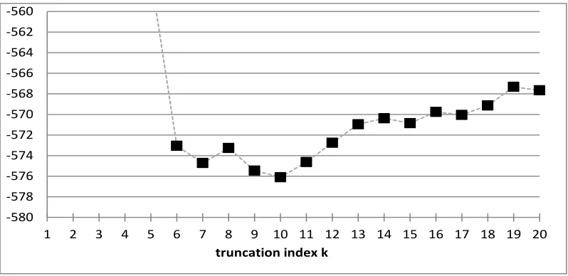
For k ∈ {1, . . . ,20} we estimate θ(k) and σ(k) using the MLE system (3.4)-(3.5) and then we calculate AIC given in formula (4.2) for each modelM(k) _{(we drop all terms coming from the} market view because at the moment we do not assume market knowledge, i.e. τj =∞). The

AICs (4.2) are provided in Figure 2. The picture confirms that the optimal truncation index for our data set is k= 10, closely followed by k= 9,7,11. Thus, the analysis explains that we should model individually the development parameters forj= 1, . . . ,9 and forj≥10 we model them by the common parameters α and β. This choice provides estimates for the intercept

b b

α(10)=−0.9060 and for the slope b b β

(10)

= 0.2497 in model M(10)_{. In Figure 3 we compare the} model where we estimate each development year j individually to the model with truncation index k = 10. We see that the straight line fitted for j ≥ 10 is close to the individual MLEs of θj, with only the last two periods j= 20,21 differing considerably. These differences should

not be over-stated because the individual estimates are based on 2 observations for j = 20 and 1 observation for j= 21, only. Moreover, the confidence bounds forj= 20,21 may also be questioned because they are based on 2 observations only, recall that we setσ2₂₁=σ₂₀2 becauseσ2₂₁

cannot be estimated from 1 observation. The latter suggests that also the variance parameters

σ2

j may be modeled by a functional form after some truncation index. For the time-being we

refrain from doing so.

6.2 Bayesian model selection with different prior knowledge

We turn to the Bayesian case where we directly work on the marginals ξDI given by Corollary

3.1. Then, we only need to estimate the standard deviation parametersσfor the different models

M(k) _{using likelihood (3.1). We first specify the prior parameters µ}(k) _{and T}(k)_{. Since for the}

-580 -578 -576 -574 -572 -570 -568 -566 -564 -562 -560

1 2 3 4 5 6 7 8 9 10 11 12 13 14 15 16 17 18 19 20

[image:18.612.100.499.71.265.2]

truncation index k

Figure 2: AIC(k) for k= 1, . . . ,20, see formula (4.2).

present example we do not have this information we make an ad-hoc choice that allows to study the sensitivities in the reliability of the prior knowledge. We choose the MLEs forµ0, . . . , µk−1 and we choose prior tail parametersµα =−1 andµβ = 0.25, the latter two choices are motivated

by the findings in the previous subsection. For T(k) we make three different choices: (1) Prior Model 1: all coefficients of variation are set equal to 1; (2) Prior Model 2: coefficients of variation of θ0, . . . , θk−1 are set equal to 0.1 and coefficients of variation of tail parameters α and β are set equal to 1; (3) Prior Model 3: all coefficients of variation are set equal to 0.1. Prior Model 1 corresponds to vague prior knowledge. Prior Models 2 and 3 put more emphasis on the prior knowledge, in Prior Model 2 we have informative prior knowledge for the individual parameters

θj and vague prior knowledge for the tail parameters ofα andβ, and in Prior Model 3 we have

informative prior knowledge for all parameters.

Finally, we assume that all models M(k) _{are equally likely a priori, resulting in the choices}

p(M(k)_{) = 1/(J−1) for k= 1, . . . , J −1. Under these assumptions we calculate the posterior} model probabilities (4.1) for the three prior information choices Prior Models 1-3, the results are presented in Figure 4. In Prior Model 2 (informative prior knowledge for θj’s and vague

prior knowledge for α and β) there is not a clear preference, truncation index k = 7 has the biggest posterior model probability of about 30% and truncation indexk= 10 receives posterior model probability of about 20%. In Prior Model 3 (informative prior knowledge for θj’s,α and

β) truncation indexesk= 9,10 are clearly favored with a posterior model probability of almost 40% each. The reason for the differences between Prior Models 2 and 3 is that in Prior Model 3 we have a pre-specified mean of µβ = 0.25 (with coefficient of variation 0.1) which fits to

models M(10) _{and M}(9)_{. Therefore, these models obtain more posterior probability weight in} Prior Model 3 compared to Prior Model 2 where the information about the prior slopeµβ has

only little credibility (and may easily be changed by observations).

For vague prior information (Prior Model 1) we clearly favor truncation indexk= 6. This might

-6.5 -6.0 -5.5 -5.0 -4.5 -4.0 -3.5 -3.0 -2.5 -2.0

0 5 10 15 20

theta MLE (individual) conf. + conf. - trunc. index k=10

Figure 3: Individual MLEsb b

θ

(k)

fork= 20 compared to the model with truncation indexk= 10.

be a small surprise because intuitively we would preferk= 7. The choicek= 6 reflects the fact that in case of little information about individual parameters we target for models with only few parameters and hence rather go for a smaller truncation indexk due to parameter uncertainty. These considerations lead to the following conclusions. If we have informative prior knowledge we choose truncation indexk= 9. If we have vague prior knowledge we try to reduce the number of parameters (to reduce parameter uncertainty) and we go for truncation indexk= 6.

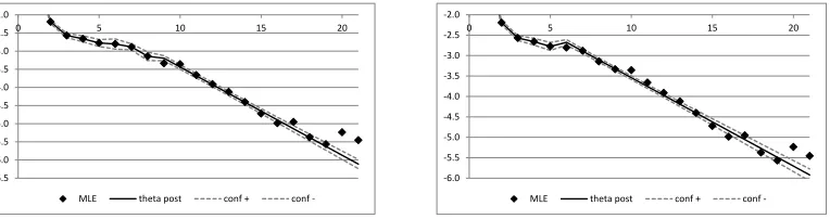
In Figure 5 we present the posterior estimates of the parameters given by

θpost(k)=E h

θ(k)

ξDI

i

=µ(k)+T(k)(A(k))0P₁0

Σ(_Ik)

−1

ξDI −µ

(k)

I

, (6.1)

which are surrounded by intervals of two posterior standard deviations obtained from the con-ditional covariance matrix

Tpost(k)= Var

θ(k)

ξDI

=T(k)−T(k)(A(k))0P₁0

Σ(_Ik)

−1

P1A(k)T(k). (6.2)

On the left-hand side (a) of Figure 5 we plot truncation indexk= 9 for Prior Model 3 and on the right-hand side (b) truncation indexk= 6 for Prior Model 1. We observe rather narrow intervals in both situations, which says that posterior parameter distributions are very concentrated. For Prior Model 1 they are slightly larger because we have more uncertainty concerning the prior knowledge. This is partly compensated by the fact that we use more observations for k= 6 to estimate the parameters of α and β compared to k = 9. These intervals for parameters mean that there is only little tail parameter uncertainty, if we believe into the truncation index model, and the dispersion in the MLEs in Figures 3 and 5 comes from process uncertainty.

6.3 Claims prediction and uncertainty analysis

Using the previous model selection analysis we calculate the predictive distribution in the lower triangleDc

I, conditionally given the upper triangleDI, see Corollary 3.2, in the selected model(s).

0% 10% 20% 30% 40% 50% 60% 70% 80% 90%

1 2 3 4 5 6 7 8 9 10 11 12 13 14 15 16 17 18 19 20

[image:20.612.100.498.81.256.2]

Prior Model 1 Prior Model 2 Prior Model 3

Figure 4: Posterior probability weights (4.1) for models M(k)_{, k = 1, . . . , J −1, for the three} different Prior Models 1-3.

-6.5 -6.0 -5.5 -5.0 -4.5 -4.0 -3.5 -3.0 -2.5 -2.0

0 5 10 15 20

MLE theta post conf + conf

--6.0 -5.5 -5.0 -4.5 -4.0 -3.5 -3.0 -2.5 -2.0

0 5 10 15 20

MLE theta post conf + conf

-Figure 5: Resulting estimates θpost(k) surrounded by intervals of two posterior standard devia-tions, see (6.1)-(6.2). (a) lhs: Prior Model 3 for truncation indexk= 9; (b) rhs: Prior Model 1 for truncation indexk= 6.

From this posterior distribution we can then calculate the best-estimate reserves and the corre-sponding conditional MSEP. Since, in general, the closed form solution is too complicated we use the simulation algorithm presented in Section 5.1. In Table 1 we present the empirical results which are based on 300’000 simulations. We first consider lines (a) and (b) of Table 1. We see that more prior information reduces prediction uncertainty (conditional MSEP of Prior Model 3 withk= 9 versus conditional MSEP of Prior Model 1 withk= 6). The resulting reserves are very similar, they are slightly higher in Prior Model 1 because its slope β of the tail parameter is slightly smaller in Prior Model 1.

Lines (c) and (d) in Table 1 correspond to the case were each development period is treated individually. We see a strong increase in the conditional MSEP. Thus, estimating each devel-opment period individually strongly increases uncertainty which is in line with the statements of over-parametrization. Moreover, we can see that prior information strongly helps to decrease

[image:20.612.112.494.359.460.2]

claims reservesRb msep_R|D I(Rb)

[image:21.612.86.517.69.171.2]

1/2 (a) Prior Model 3, truncation index k= 9 1’438’947 52’090 (b) Prior Model 1, truncation index k= 6 1’440’738 53’321 (c) Prior Model 3, individual development periods 1’485’416 59’816 (d) Prior Model 1, individual development periods 1’492’284 68’240 (e) Bayesian ODP model of Verrall-W¨uthrich [14] 1’476’301 54’073

Table 1: Resulting best-estimate claims reservesRband corresponding conditional MSEP for (a)

Prior Model 3 with truncation index k= 9 and (b) Prior Model 1 with truncation index k= 6. These are compared to the best-estimate claims reserves and the conditional MSEP if we model each development period individually in (c) Prior Model 3 and (d) Prior Model 1, respectively, and to (e) the Bayesian ODP model of Verrall-W¨uthrich [14], Table 4.

uncertainty, line 3 versus line 4 in Table 1. We also observe that the resulting best-estimate claims reserves are higher in the individual development period modeling approach compared to the truncation index model. This comes from the fact that the truncation index model judges the tail decay more favorably for our data set, see Figure 5.

If we compare these results, given in Table 1, to the Bayesian over-dispersed Poisson (ODP) model of Verrall-W¨uthrich [14], Table 4, we see that they are quite similar. With comparable prior uncertainty as in Prior Model 3, we choose truncation index k= 7 in the Bayesian ODP model and the resulting reserves and uncertainties are rather similar to our model (though the model assumptions are very different). Again, our model has the advantage over the Bayesian ODP model that we do not need involved RJMCMC simulations, see Section 3 of Verrall-W¨uthrich [14], but obtain model selection and posterior parameters analytically.

Figure 6: Resulting empirical density (red histogram) and Gaussian approximation (blue line). (a) lhs: Prior Model 3 for truncation indexk= 9; (b) rhs: Prior Model 1 for truncation index

k= 6.

In Figure 6 we plot the resulting empirical density and the corresponding Gaussian approxima-tion using Rb and msep_R|D

I(Rb) for fitting the first two moments of the Gaussian distribution. 3

[image:21.612.90.488.504.624.2]

[image:22.612.101.495.112.280.2]

At the first sight, the Gaussian approximations in Figure 6 seem to fit very well. In Figure 7

Figure 7: lhs: log-log plot of the empirical survival distributions x7→P[R > x|DI] for (a) Prior

Model 3 for truncation index k= 9 and (b) Prior Model 1 for truncation index k= 6, the line gives the Gaussian approximation; rhs: densities of the 4 models (a)-(d) of Table 1.

(lhs) we present the log-log plot of the empirical survival distributions x 7→ _P[R > x|D_I] for models (a) and (b) of Figure 6. We see that in the tails the Gaussian approximation clearly underestimates the potential of large losses because it is less heavy tailed than the distribution of R (which is driven by log-normal distributions).

In Figure 7 (rhs) we plot the resulting empirical densities of models (a)-(d) presented in Table 1. We see that (a) and (b) provide similar results. If we model every development period individually, see models (c) and (d), we obtain the shift seen in Table 1. This shift comes from the fact that the observations for j = 20,21 receive more weight in the latter models, see Figure 5; depending on the data the sign could also go into the other direction. More interestingly, we see that the density is more widely spread the less information we have and the more parameter we have: the least uncertain prediction is obtained in Prior Model 3 with truncation index k = 9, the most uncertain in Prior Model 1 with every development period modeled individually. The shift in claims reserves from models (a)-(b) to models (c)-(d) may raise the question whether the tail decay is judged too optimistically under an exponential decay model (since the claims reserves from the individual MLEs modeling are more conservative). In Figure 8 we include in addition to Figure 5 also confidence bounds for the MLEs (symmetric around the posterior estimate θpost(k)). We observe large volatilities in these MLEs for large development year indexesjand, thus, our model about the exponential decay cannot be rejected in view of Figure 8 because the MLEs are all within the confidence bounds. We also see that the estimates of σ could be smoothed to obtain more monotonicity in the confidence bounds. Nevertheless, if the exponential decay is too fast, we could also try to fit a power decay of the form

exp{α}j−β = exp{α−βlogj}. (6.3)

-6.5 -6.0 -5.5 -5.0 -4.5 -4.0 -3.5 -3.0 -2.5 -2.0

0 5 10 15 20

MLE theta post conf param + conf param - conf MLE + conf MLE

--6.5 -6.0 -5.5 -5.0 -4.5 -4.0 -3.5 -3.0 -2.5 -2.0

0 5 10 15 20

MLE theta post conf param + conf param - conf MLE + conf MLE

-Figure 8: Resulting estimates θpost(k) with corresponding intervals of two standard deviations, see (6.1)-(6.2). (a) lhs: Prior Model 3 for truncation index k = 9; (b) rhs: Prior Model 1 for

truncation indexk= 6. The weak dotted lines are the confidence bounds for the MLEsb b

θ

(20) .

claims reserves Rb approximationRbapprox

[image:23.612.96.498.90.192.2]

(a) Prior Model 3, truncation indexk= 9 1’438’947 1’438’886 (b) Prior Model 1, truncation indexk= 6 1’440’738 1’440’545

Table 2: Resulting best-estimate claims reserves Rb and approximation Rbapprox for (a) Prior

Model 3 with truncation indexk= 9 and (b) Prior Model 1 with truncation indexk= 6.

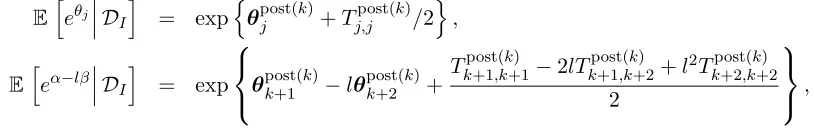
Next we study the first order approximation (and lower bound) presented in Section 5.2, see (5.4). In view of (6.1)-(6.2) we obtain for j < k and l≥k

E h

eθj DI

i

= exp

n

θpost(_j k)+T_j,jpost(k)/2

o ,

E h

eα−lβ DI

i

= exp

 



θpost(_k+1 k)−lθpost(_k+2k)+T post(k)

k+1,k+1−2lT post(k)

k+1,k+2+l2T post(k)

k+2,k+2 2

 

 ,

where θpost(_l k) is the l-th component of θpost(k) and T_l,mpost(k) is element (l, m) of covariance matrixTpost(k). This allows approximationRbapprox=

P

iRbapprox_i given by (5.4) to be calculated

explicitly. In Table 2 we present the corresponding results. We observe that the two values are very close (which also verifies that the simulation algorithm presented in Section 5.1 was implemented correctly).

6.4 Tail factors

Finally, we study the inclusion of tail factors according to Section 5.3. In our example J∞= 50

is sufficient for capturing the tail, this can be seen by expanding/approximating the tail as in the first order approximation (5.4).

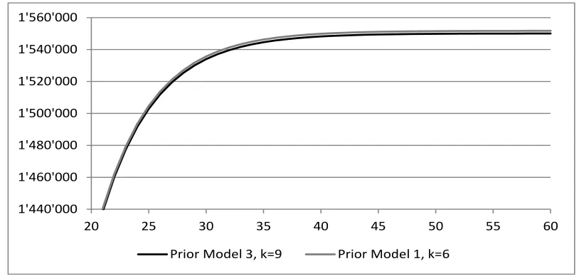
In Figure 9 we plot the resulting reserves Rbult = P

iRbult_i as a function of J∞, which justifies

the choiceJ∞= 50. In a similar way to Section 5.1 we simulate paymentsCi,J∞,i∈ {1, . . . , I},

which allow to quantify tail prediction uncertainty within our model M(k)_{. The results are} presented in Table 3. We observe that the predicted claims payments beyond the last observed

[image:23.612.94.501.433.499.2]

1'440'000 1'460'000 1'480'000 1'500'000 1'520'000 1'540'000 1'560'000

20 25 30 35 40 45 50 55 60

[image:24.612.94.501.72.266.2]

Prior Model 3, k=9 Prior Model 1, k=6

Figure 9: Claims reservesRbult= P

iRbult_i as a function ofJ∞= 21, . . . ,60 for (a) Prior Model 3

with truncation indexk= 9 and (b) Prior Model 1 with truncation indexk= 6.

reservesRb msep_R|D I(Rb)

1/2 _reserves

b

Rult cond. MSEP (a) Prior Model 3, k= 9 1’438’947 52’090 1’527’078 55’635 (b) Prior Model 1, k= 6 1’440’738 53’321 1’552’331 58’950

Table 3: (a) Prior Model 3 with truncation index k= 9 and (b) Prior Model 1 with truncation index k = 6: best-estimate claims reserves Rb and best-estimate claims reserves Rbult including

tail factors and corresponding conditional MSEPs forJ∞= 50.

development period J = 21 add an additional 7% to the claims reservesRb. Model (b) is more

conservative about this tail development, this comes from the fact that the slope E[β|DI] is

smaller in Model (b), i.e. 0.22 versus 0.24 in Model (a). The increase in uncertainty (conditional MSEP) is almost 10%. Finally, in Figure 10 we present the corresponding log-log plot and the densities.

7

Conclusion

We consider a Bayesian log-normal model for claims reserving in a chain-ladder framework. We assume that there is a fixed truncation index. Each development period before this truncation index is assumed to have an individual parameter, and development periods after the truncation index are assumed to have a common functional form. We explain how this model can be fit to data and how model selection w.r.t. the truncation index can be done. The advantage of our Bayesian log-normal model is that we do not need involved reversible jump Markov chain Monte Carlo simulation methods as, for instance, used in Verrall-W¨uthrich [14]. Once this model is fit to the data, the common functional form above the truncation index gives a natural way to

[image:25.612.106.495.83.259.2]

Figure 10: lhs: log-log plot of the survival distributions x7→_P[Rult> x|D_I] for (a) Prior Model 3 for truncation index k= 9 and (b) Prior Model 1 for truncation index k = 6, the line gives the Gaussian approximations; rhs: densities of the 2 models (a) and (b) of Table 3.

estimate tail factors beyond the latest observed development delay.

References

[1] Akaike, H. (1974). A new look at the statistical model identification. IEEE Transactions on Auto-matic Control 19/6, 716-723.

[2] Boor, J., (2006). Estimating tail development factors: what to do when the triangle runs out. CAS Forum Winter 2006, 345-390.

[3] B¨uhlmann, H., Gisler, A. (2005). A Course in Credibility Theory and its Applications. Springer.

[4] De Jong, P., Zehnwirth, B. (1983). Claims reserving, state-space models and the Kalman filter.

Journal Institute Actuaries 110, 157-182.

[5] England, P.D., Verrall, R.J. (2001). A flexible framework for stochastic claims reserving. Proc. CAS,

Vol. LXXXVIII, 1-38.

[6] Gigante, P., Picech, L., Sigalotti, L. (2013). Prediction error for credible claims reserves: an h

-likelihood approach. European Actuarial Journal 3/2, 453-470.

[7] Hertig, J. (1985). A statistical approach to the IBNR-reserves in marine insurance. Astin Bulletin

15/2, 171-183.

[8] Johnson, R.A., Wichern, D.W. (1988). Applied Multivariate Statistical Analysis. 2nd edition.

Prentice-Hall.

[9] Lee, Y., Nelder, J.A. (1996). Hierarchical generalized linear models. Journal Royal Statistical Society

B 58/4, 619-678.

[10] Lee, Y., Nelder, J.A. (2001). Hierarchical generalised linear models: a synthesis of generalised linear

models, random-effects models and structured dispersions. Biometrika 88/4, 987-1006.

[11] Merz, M., W¨uthrich, M.V., Hashorva, E. (2013). Dependence modelling in multivariate claims run-off triangles. Annals of Actuarial Science 7/1, 3-25.

[12] Shi, P., Basu, S., Meyers, G.G. (2012). A Bayesian log-normal model for multivariate loss reserving. North American Actuarial Journal 16/1, 29-51.

[13] Verrall, R.J. (1996). Claims reserving and generalised additive models. Insurance: Mathematics & Economics 19/1, 31-43.

[14] Verrall, R.J., W¨uthrich, M.V. (2012). Reversible jump Markov chain Monte Carlo method for pa-rameter reduction in claims reserving. North American Actuarial Journal 16/2, 240-259.

[15] W¨uthrich, M.V. (2012). Discussion of ”A Bayesian log-normal model for multivariate loss reserving” by Shi-Basu-Meyers. North American Actuarial Journal 16/3, 398-401.

[16] W¨uthrich, M.V. (2013). Non-Life Insurance: Mathematics & Statistics. SSRN Manuscript ID 2319328.

[17] W¨uthrich, M.V., Merz, M. (2008). Stochastic Claims Reserving Methods in Insurance. Wiley.