City, University of London Institutional Repository
Citation:
Owadally, I. & Landsman, Z. (2013). A characterization of optimal portfolios under the tail mean-variance criterion. Insurance: Mathematics and Economics, 52(2), pp. 213-221. doi: 10.1016/j.insmatheco.2012.12.004This is the submitted version of the paper.
This version of the publication may differ from the final published
version.
Permanent repository link:
http://openaccess.city.ac.uk/17092/Link to published version:
http://dx.doi.org/10.1016/j.insmatheco.2012.12.004Copyright and reuse: City Research Online aims to make research
outputs of City, University of London available to a wider audience.
Copyright and Moral Rights remain with the author(s) and/or copyright
holders. URLs from City Research Online may be freely distributed and
linked to.
City Research Online: http://openaccess.city.ac.uk/ publications@city.ac.uk
A Characterization of Optimal Portfolios under the Tail
Mean-Variance Criterion
Iqbal Owadallya,∗
, Zinoviy Landsmanb,∗∗
a
Faculty of Actuarial Science and Insurance, Cass Business School, City University London, 106 Bunhill Row, London EC1Y 8TZ, United Kingdom
b
Department of Statistics, University of Haifa, Mount Carmel, 31905 Haifa, Israel
Abstract
The tail mean-variance model was recently introduced for use in risk management and
portfolio choice, and involves a criterion that focuses on the risk of rare but large losses,
which is particularly important when losses have heavy-tailed distributions. If returns
or losses follow a multivariate elliptical distribution, the use of risk measures that satisfy
certain well-known properties is equivalent to risk management in the classical
mean-variance framework. The tail mean-mean-variance criterion does not satisfy these properties,
however, and the precise optimal solution typically requires the use of numerical methods.
We use a convex optimization method and a mean-variance characterization to find an
explicit and easily implementable solution for the tail mean-variance model. When a
risk-free asset is available, the optimal portfolio is altered in a way that differs from the classical
mean-variance setting. A complete solution to the optimal portfolio in the presence of a
risk-free asset is also provided.
Keywords: Tail conditional expectation, Tail variance, Optimal portfolio selection, Quartic equation
JEL: G11, Classification: IM12 IE13 IB63
∗Corresponding author. Email: m.i.owadally@city.ac.uk. Phone: +44 (0)20 7040 8478. Fax: +44 (0)20 7040 8572.
1. Introduction
In this paper, we consider portfolio selection under the tail mean-variance criterion that
was introduced by Landsman (2010):
T M V(L) = E[L|L >VaRq(L)] + λVar [L|L >VaRq(L)]. (1)
In the above, (i) λ > 0, (ii) L is a random loss, with a continuous distribution, on a
portfolio, (iii) VaRq(L) is the value-at-risk on the portfolio and is defined as
VaRq(L) = inf(x∈R:FL(x)≥q), (2)
where q ∈ (0,1) and FL(x) is the cumulative distribution function of loss L. (q = 0.95
therefore corresponds to a 5% value-at-risk.) The objective is to find an optimal portfolio
that minimizes the tail mean-variance criterion subject to a budget constraint.
Since portfolio return R =−L, the tail mean-variance criterion may be regarded as an analogue of the classical mean-variance criterion (see e.g. Panjer et al., 1998, p. 379):
M V(L) = EL + 1
2τVarL = −ER + 1
2τVarR, (3)
with τ >0. This originates from the mean-variance portfolio theory of Markowitz (1952),
of course. Unlike its classical counterpart, the tail mean-variance criterion focuses on the
behaviour of the tail of portfolio returns through the q-quantile specified in the
value-at-risk. This is of interest to portfolio managers whose clients may be concerned with portfolio
performance in the event of extreme losses on capital markets.
We make three significant contributions in this paper. First, we use a convex
optimiza-tion method to find an explicit and easily implementable soluoptimiza-tion for tail mean-variance
optimization. We retain the assumption of joint elliptically distributed returns on securities
but, unlike the solution of Landsman (2010), our solution is simple and avoids a sequence
of matrix partitions and manipulations. The matrices may be of a large dimension for
portfolios containing many hundred securities and involving a large variance-covariance
matrix, so our solution has a considerable computational advantage. Secondly, our
for the tail mean-variance optimal portfolio in terms of mean-variance efficiency. This
facil-itates comparison with optimal portfolios under other criteria, such as the mean-variance
and value-at-risk criteria. Thirdly, we further extend the work of Landsman (2010) by the
inclusion of risk-free lending and borrowing. A complete, closed-form optimal solution is
provided.
It is convenient to introduce at this point some notation and assumptions used in
the rest of the paper. R, R+ and R++ denote the sets of real numbers, real non-negative
numbers and real positive numbers respectively. We assume that there arenrisky securities
with mean returnµ∈Rn and variance-covariance matrix Σ∈Rn×n. Define 0and 1to be
column vectors of zeros and ones respectively, of dimensionn. As is usual, we assume that
µis not collinear with1, i.e. that securities do not all have the same mean return, and that
Σ is a (symmetric) positive definite and non-singular matrix. Let x∈Rn be the vector of
proportions of wealth invested in a portfolio. Define P as the set of feasible portfolios of risky securities only:
P = {x∈Rn :1Tx= 1}. (4) We assume in the above that all wealth is invested. In section 6, a risk-free asset is included,
in which case the proportion of wealth invested in the risk-free asset is 1−1Tx. There is no constraint other than the budget constraint that all wealth be invested and, in particular,
short sales are allowed.
The plan of this paper is as follows. The motivation and literature related to this paper
are described in section 2. In section 3, we briefly review some results on the tail conditional
expectation, the tail variance, and on the tail mean-variance criterion. A characterization of
the optimal portfolio under the tail mean-variance criterion using mean-variance efficiency
is discussed in section 4. A novel solution for the tail mean-variance optimal portfolio is
derived in section 5 when portfolios consist of risky securities only. It is illustrated with
the help of a numerical example. When risk-free lending and borrowing are introduced,
the tail mean-variance optimal portfolio is altered and this is detailed in section 6. A few
2. Background and Related Literature
There are two strands in the development of work related to portfolio optimization. One
strand concerns multi-period optimal portfolio selection, initiated by Merton (1969, 1971).
Security prices are modelled as continuous-time random processes based on geometric
Brownian motion: see Karatzas and Shreve (1991), Yang and Zhang (2005) and Chacko
and Viceira (2005) among others. A recent and significant development in this direction is
made by Zhao and Rong (2012) who assume investment in multiple risky assets under the
constant elasticity of variance (CEV) model with stochastic volatility. This generalizes the
geometric Brownian motion model where volatility is deterministic.
In this paper, we choose to follow the second strand of portfolio optimization, namely
single-period optimization originally due to Markowitz (1952). There are several reasons
why we make this choice. First, the single-period mean-risk model is routinely used in
the investment industry because it allows for practical trading constraints, frictional costs
and similar realistic issues. We endeavor in this paper to add to the level of sophistication
that may be applied to such models. Secondly, parameter and model mis-specification
risks are very significant in practical portfolio management. The one-period model can
accommodate these, for example through a Bayesian approach (see e.g. Garlappi et al.,
2007; Tu and Zhou, 2004; Kan and Zhou, 2007), in a way which is readily implementable
by practitioners. We supply a closed-form solution in the single-period model which may
in future be extended to allow greater robustness. Thirdly, the effect of inter-temporal
hedging is typically small, so that optimal portfolios in the dynamic setting are often
(but not always) close to those in the static setting (Chacko and Viceira, 2005). Finally,
both individual and institutional investors are concerned with downside and tail risks in
portfolio returns, and traditional models fail to capture this. We are able to obtain explicit
expressions for optimal portfolios in the one-period setting taking tail risk into account.
In order to solve for tail mean-variance optimal portfolios, we also leverage recent
findings on risk measures. Indeed, the tail mean-variance criterion may be viewed as a
is the tail conditional expectation of losses, which is identical to the expected shortfall
risk measure since losses are assumed to be continuously distributed (see e.g. McNeil,
Frey and Embrechts, 2005, p. 45). Acerbi and Tasche (2002) show that the tail conditional
expectation satisfies a set of acceptable properties for risk measures and is therefore deemed
to be a coherent risk measure in the sense of Artzner et al. (1999). The second term on
the right hand side of equation (1) represents the tail variance, proposed by Furman and
Landsman (2006).
Notice that the tail conditional expectation is the best estimate, in a least squares sense,
of the worst losses on a portfolio, when losses larger than the q-quantile are considered:
E[L|L >VaRq(L)] = arg inf w E
(L−w)2
|L >VaRq(L)
. (5)
On the other hand, the tail variance of Furman and Landsman (2006) gives the estimated
squared deviation of the worst losses from the tail conditional expectation:
Var [L|L >VaRq(L)] = inf w E
(L−w)2
|L >VaRq(L)
. (6)
The tail conditional expectation is explicitly calculated for multivariate distributions that
are normal, elliptical, gamma, Pareto and for exponential dispersion models by Panjer
(2002), Landsman and Valdez (2003), Furman and Landsman (2005), Chiragiev and
Lands-man (2007) and LandsLands-man and Valdez (2005) respectively. FurLands-man and LandsLands-man (2006)
calculate the tail variance in the case of multivariate normal distributions and, more
gen-erally, elliptical distributions.
3. Results on Tail Conditional Expectation and Tail Variance
We start by briefly reviewing some known results on spherical and elliptical distributions
and their application to risk management.
If z : Ω →Rn is spherically distributed with characteristic generator ψ, then its
char-acteristic function is a function of the Euclidean norm of t, wheret∈Rn is the argument of the characteristic function:
ϕz(t) = Eexp itTz = ψ
1 2||t||
2
ψ is termed the characteristic generator because it specifies different members of the
spher-ical family of distributions. For example, the standard normal random variable has
char-acteristic function exp (−t2/2).
Elliptical distributions are affine transformations of spherical distributions, so that
probability density contours are distorted from spheroids to ellipsoids. Let r: Ω→Rn be a vector of asset returns on n securities. Ifr is elliptically distributed with location vector
µ∈Rn, dispersion matrix Σ∈Rn×nand characteristic generatorψ, then its characteristic
function is
ϕr(t) = Eexp itTr = exp itTµ ψ
1 2t
T Σt
. (8)
For further details on spherical and elliptical distributions, see Fang et al. (1990).
A key property of elliptically distributed random variables with the same characteristic
generator ψ is that any linear combination of these random variables is also elliptically
distributed with the same characteristic generator. This is easily established from
equa-tion (8). Thus, the return xTr on a portfolio x is elliptically distributed with mean
µTx,
variance xTΣxand characteristic generatorψ, assuming that the mean and variance exist
(Owen and Rabinovitch, 1983).
Landsman and Valdez (2003) show that, when returns are jointly elliptically distributed,
the tail conditional expectation of portfolio loss, based on the q-quantile, may be written
as
E[L|L >VaRq(L)] = −µTx + λ1,q
√
xTΣx, (9)
since L=−xTr. The parameter λ1
,q is uniquely specified by q:
λ1,q = hZ,Z∗(zq), (10)
where hZ,Z∗(z) = fZ∗(z)/FZ(z) is a distorted hazard rate evaluated at the q-quantile of
the standardized random variable Z = (r1 − µ1)/√σ11. Here, FZ(z) = 1 − FZ(z) is
the decumulative distribution function of Z whereas FZ(z) is the cumulative distribution
function of Z; the first element of r is r1 with mean µ1 =Er1 and variance σ11= Var(r1);
and fZ∗(z) is the density of some spherical random variable Z ∗
is called the distribution associated with the elliptical family (see Landsman and Valdez,
2003, for details).
The corresponding tail variance, when returns are elliptically distributed, is derived by
Furman and Landsman (2006):
Var [L|L >VaRq(L)] = λ2,qxTΣx. (11)
The parameter λ2,q is also uniquely specified by q:
λ2,q = r(zq) +hZ,Z∗(zq)(zq−hZ,Z∗(zq)), (12)
wherer(z) = FZ∗(z)/FZ(z) and is also evaluated at the q-quantile ofZ, and FZ∗(z) is the
decumulative distribution function of Z∗
.
In view of equations (9) and (11), the tail mean-variance criterion of equation (1) may
be written as (Landsman, 2010):
f(x;λ, q) = −µTx + λ1,q
√
xTΣx + λλ2
,qxTΣx. (13)
We may write the tail mean-variance criterion more succinctly asf(x) where this causes no
confusion. The two parameters of the tail mean-variance criterion describe an investor’s risk
preferences. The first parameter, λ ∈ R++, can be regarded as a risk aversion parameter
and is akin to τ in the classical mean-variance criterion of equation (3). The larger λ,
the more risk-averse an investor is, and the larger the additional return they expect as
a compensation for a unit increase in the variance of their portfolio return. The second
parameter, q ∈ (0,1), defines a certain threshold of loss on the portfolio. A tail
mean-variance-optimizing investor is sensitive to losses beyond the q-quantile. These are losses
which are typically rare but large.
4. Characterization of the Tail Mean-Variance Optimal Portfolio
4.1. Classical Mean-Variance Criterion
It is well-known that, when returns or losses follow a multivariate elliptical distribution,
expectation is equivalent to the use of the classical mean-variance framework. This is
highlighted by McNeil, Frey and Embrechts (2005), with an emphasis on the
value-at-risk measure. More specifically, Proposition 6.13 of McNeil, Frey and Embrechts (2005,
p. 247) shows that an investor who wishes to achieve a target expected return will choose
the same optimal portfolio whether his measure of risk is the variance, the value-at-risk
or any other measure that satisfies the properties of translation invariance and positive
homogeneity. (See Artzner et al. (1999) for properties of coherent risk measures.) It
is clear from equation (1) that the tail mean-variance criterion does not satisfy positive
homogeneity: T M V(kL)6=k×T M V(L) for k >0. Nevertheless, we shall show that the tail variance criterion, under multivariate elliptical risks, does revert to the
mean-variance setting.
To this end, consider the classical mean-variance criterion
g(x;τ) = −µTx + 1
2τx T
Σx, (14)
which corresponds to equation (3). g(x;τ) expresses a risk-averse investor’s tradeoff
be-tween expected portfolio returnµTxand variance of portfolio returnxTΣx, through a risk
aversion parameter τ >0. Such an investor seeks to minimize g(x;τ) subject to a budget
constraint such as 1Tx = 1.
The minimization of g(x) wrt x∈ P is straightforward (see e.g. Panjer et al., 1998, p.
382) and results in the optimal solution
x = x0+ 1
τz (15)
where
x0 = 1TΣ
−1
1−1Σ−1
1, (16)
z = Σ−1
µ − 1TΣ−1µ 1TΣ−11 −1
Σ−1
1. (17)
x0 ∈ P is the global minimum variance portfolio, i.e. the portfolio that minimizes xTΣx subject to 1Tx = 1. As for z
The concept of efficient frontiers is natural in mean-variance optimization. We employ
the usual definition of mean-variance efficiency that is found in textbook treatments of
portfolio theory, e.g. in Panjer et al. (1998, p. 379): a portfolio xis called (mean-variance)
efficient if there exists no portfolio x1 with µTx1 ≥ µTx and x1TΣx1 < xTΣx. The
mean-variance efficient frontier E is then the set of portfolios defined by
E = {x0} ∪ {x∈Rn: x = arg min
x∈P
g(x;τ) for each τ ∈R++}. (18)
At this stage we collect some statistical properties about the returns of x,x0 andz, as
they will be useful later. Recall throughout that Σ is a real, positive definite, symmetric,
non-singular matrix.
It is well-known (see e.g. Lee and Lee, 2006, p. 458) that the return on the global
mean-variance portfolio x0 in equation (16) has the same covariance with the return on all
non-self-financing portfolios x∈ P (for which1Tx= 1), including itself:
xTΣx0 = 1TΣ
−1
1−1
xT1 = 1TΣ−1
1−1
= x0TΣx0. (19)
But the return onx0 also has zero covariance with the return on the self-financing portfolio
z of equation (17) (for which1Tz= 0):
zTΣx0 = 1TΣ
−1
1−1zT1 = 0. (20)
The mean return on the global mean-variance optimal portfolio is proportional to its
vari-ance:
µTx0 = µTΣ
−1
1 1TΣ−1
1−1 = µTΣ−11 x0TΣx0
(21)
in view of equation (19).
Turning to the self-financing portfolio z of equation (17), and comparing it with x0 in
equation (16), we find that z= Σ−1
µ−(1TΣ−1µ)x0, so that its mean return is
µTz = µTΣ−1µ−(1TΣ−1µ)µTx0, (22)
which equals its variance of return since
zTΣz = µTΣ−1µ−2(1TΣ−1µ)µTx0+ (1TΣ
−1
µ)2x0TΣx0 = µTΣ−1µ−(1TΣ−1µ)µTx0.
ReplacingµTx0 from equation (21) into equation (22) results in an expression for the mean
and variance of the return on the self-financing portfolio:
µTz = zTΣz = h
µTΣ−1µ 1TΣ−11 − 1TΣ−1µ
2i
1TΣ−1
1−1. (24)
Finally, from equations (15), (19), (20) and (23), we find that the variance of return on
the mean-variance optimal portfolio is:
xTΣx = x0TΣx0+ 1 τ2z
T
Σz+2 τx0
T
Σz = 1TΣ−1
1−1 + 1 τ2µ
T
z. (25)
4.2. Tail Mean-Variance Criterion
Landsman (2010) shows that the tail mean-variance optimal portfolio that minimizes
f(x) (in equation (13)) subject to 1Tx= 1 is
x∗ = arg min
x∈P
f(x) = x0+ w∗
ℓ u. (26)
In the above, x0 is the global minimum variance portfolio of equation (16), and ℓ and u
are functions of mean µ and covariance Σ of stock returns. The functions ℓ and u are
fairly complicated and involve partitioned matrices and their inverses and they are not
reproduced here: see Landsman (2010) for details. As for w∗
, it is the unique real root
within the interval (0, ℓ/2λλ2,q) of the following quartic equation:
w4
− λλ2ℓ
,q
w3 +
1TΣ−1
1−1 + ℓ 2
−λ2 1,q
(2λλ2,q)2
w2
−ℓ 1 T
Σ−1
1−1
λλ2,q
w+ℓ2 1 T
Σ−1
1−1
(2λλ2,q)2
= 0
(27)
Our aim is to explain the form of x∗
, relate it to mean-variance efficient portfolios, and
simplify its calculation. The following two lemmas are useful in proving our main theorem.
Lemma 1. Assume q ∈(0,1). Then λ1,q >0 and λ2,q >0.
Proof. λ1,q is a ratio of probability density and decumulative probability in equation (10).
λ2,q >0 follows immediately from equation (11).
See Landsman (2010) for a proof. The mean µTx and variance xTΣx are continuous
on P, and so is f(x). On the r.h.s. of equation (13), xTΣx is strictly convex on
Rn and −µTxis convex (linear), while the coefficients λ1,q andλλ2,q are positive by Lemma 1. So
one only needs to show that √xTΣxis convex on Rn, rather than strictly convex.
A consequence of Lemma 2 is thatf(x) has at most one minimum onP. The following lemma characterizes this minimum if it exists.
Lemma 3. Assume that there exists a portfolio x∗
= arg minx∈Pf(x). Then x∗ ∈ E.
Proof. We wish to show that x∗
= arg minx∈Pf(x) ⇒ x∗ = arg minx∈Pg(x;τ0) for some
τ0 > 0. Proof by contradiction: Suppose that x∗
= arg minx∈Pf(x) and x∗ 6=
arg minx∈Pg(x;τ0). Then there exists a portfolio x1 ∈ P with g(x1;τ0) < g(x∗;τ0)
such that µTx1 ≥ µTx∗ and x1TΣx1 < x∗TΣx∗. In equation (13), λ > 0 by defi-nition and λ1,q, λ2,q > 0 by virtue of Lemma 1. Therefore, f(x1) < f(x∗). But then
x∗
6
= arg minx∈Pf(x), which is a contradiction.
The proof of Lemma 3 is simple enough, but it is illuminating to rewrite the tail
mean-variance criterion in equation (13) as follows:
f(x) = −µTx+λλ2,q
√
xTΣx+ λ1,q 2λλ2,q
2
− λ
2 1,q
4λλ2,q
. (28)
Note that λλ2,q > 0, λ1,q/2λλ2,q > 0 by Lemma 1. For
√
xTΣx > 0, the quadratic
√
xTΣx+λ1
,q/2λλ2,q
2
is monotonically increasing in √xTΣx, and therefore in xT Σx,
Thus, holding the mean of portfolio return constant, minimizing f(x) is equivalent to
minimizing the variance of portfolio return.
Based on Lemma 3, it would not be surprising if the tail mean-variance optimal portfolio
solution x∗
has the same form as the mean-variance optimal portfolio x. Comparing the
solution x∗
of Landsman (2010) in equation (26) to x in equation (15), we find that they
do indeed bear a strong resemblance in that they both involve an adjustment to the global
5. Tail Mean-Variance Optimization with Risky Securities Only
5.1. Optimization
If a tail mean-variance-optimizing investor has a given target expected return, then
his optimal portfolio is readily calculated using standard methods as it lies on the
mean-variance efficient frontier. This is indeed also true of investors who have a target expected
return and wish to minimize a translation-invariant and positive-homogeneous risk
mea-sure, as stated in Proposition 6.13 of McNeil, Frey and Embrechts (2005, p. 247). However,
if there is no given target expected return, and if the investor wishes to freely optimize the
tail mean-variance criterion of equation (1), the precise optimal solution is not so easily
calculated and would typically be found using numerical methods. Nevertheless,
Lands-man (2010) obtained an analytic solution and our aim in this section is to shed some light
on this solution and to simplify it.
Before proving our main theorem, we establish a simple lemma on quartic polynomials.
As will become apparent later, this lemma means that we do not need to be concerned
with the algebraic solution of quartic equations.
Lemma 4. The quartic polynomialF(x) = (x−a)2(x2+b)
−cx2 witha, b, c >0has exactly
one non-coincident real zero in (0, a) and exactly one non-coincident real zero in (a,∞).
See Appendix A.1 for a proof of the above. The following theorem contains our main
result.
Theorem 1. The minimum of f(x;λ, q) in equation (13) wrt x∈ P exists and is unique and occurs at
x∗ = x0+ 1
τ∗z, (29)
where x0 andz are given in equations (16) and (17) respectively, and τ∗ ∈Ris the unique
root of the quartic equation
(τ −2λλ2,q)2
h
1TΣ−1
1−1
τ2
+µTz i
− τ2 λ2
1,q = 0 (30)
Proof. Define the Lagrangian Lf(x, γf) = f(x)−γf(1Tx−1) where γf ∈Ris a Lagrange
multiplier. ∂Lf/∂x=0 and ∂Lf/∂γf = 0 may be written as
µ−
λ1,q
√
xTΣx+ 2λλ2,q
Σx+γf1 = 0, 1Tx= 1. (31)
Suppose that the solution to the equation set (31) exists and denote it by (x∗
, γ∗
f).
Consider instead the mean-variance optimization problem with g(x) defined in
equa-tion (14). Define the Lagrangian Lg(x, γg) =g(x)−γg(1Tx−1) whereγg ∈R is another
Lagrange multiplier. The optimal solution (x, γg) is the solution to
µ−τΣx+γg1 = 0, 1Tx= 1. (32)
Now, the solution (x∗, γ∗
f) of equation system (31) coincides with the solution (x, γf)
of equation system (32) provided that τ takes a specific value, denoted byτ∗
, such that
τ∗ = √ λ1,q
(x∗TΣx∗)+ 2λλ2,q =
λ1,q
√
xTΣx + 2λλ2,q. (33)
The existence of x∗
depends on the existence of a solution for τ∗
∈ R++ in the above equation.
Substituting xTΣx from equation (25) into equation (33) and rearranging yields
τ∗
−2λλ2,q =
τ∗
λ1,q
√
(1TΣ−11)−1+
µTz
, (34)
which can also be rewritten as the quartic equation (30). In equation (34), λ1,q > 0 and
2λλ2,q > 0 by Lemma 1, and 1TΣ−11 > 0 by positive definiteness of Σ. Furthermore,
µTz > 0 because µTz = zTΣz from equation (23) and Σ is positive definite and z 6= 0.
(µTz >0 also follows from the Cauchy-Schwarz inequality on the r.h.s. of equation (24).)
Since τ∗
∈R++, the r.h.s. of equation (34) is positive and real, and so should be the l.h.s. Thus, τ∗
>2λλ2,q. Lemma 4 confirms the existence of a unique real root of equation (30)
in the range (2λλ2,q,∞), which also serves to confirm the existence of x∗ =x with τ =τ∗
in equation (15). Finally, uniqueness of the minimum atx∗
5.2. Practical Advantages and Comparison with Previous Solution
Some remarks about Theorem 1 are in order. First, the optimal portfolio x∗
in
equa-tion (29) corresponds to the original soluequa-tion in equaequa-tion (26) derived by Landsman (2010),
but has a much simpler form. In particular, the quartic equation (30) corresponds to the
original quartic equation (27) but is simpler.
Secondly, Theorem 1 is markedly easier to implement than the original solution of
Landsman (2010). The cumbersome functions ℓ and u in equation (26) do not arise,
and successive matrix partitions, concatenations and inversions are avoided. For practical
investment purposes, a large number of securities is likely to be held in a portfolio. Our
solution speeds up considerably the computation of optimal portfolios when there are a
large number of securities, involving large covariance matrices.
Thirdly, portfolio optimization is known to be sensitive to parameter and model
mis-specification risks (see e.g. Tu and Zhou, 2004; Kan and Zhou, 2007). The simplified
optimal portfolio in equation (29) means that sensitivity analysis is feasible and more
straightforward. A portfolio manager can investigate different portfolios as parameters
change. In particular, the change in the optimal portfolio under different multivariate
elliptical distributions, capturing increasing or decreasing dependence in the tail, can be
measured. The construction of robust portfolios, for example incorporating Bayesian priors,
can also be contemplated (see e.g. Garlappi et al., 2007).
Fourthly, the original proof of Landsman (2010) proceeds by laborious substitution of
the portfolio budget constraint into the tail mean-variance optimization objective of
equa-tion (13). Our proof involves an elegant use of the Lagrangian multiplier and a comparative
analysis with another optimization problem. The solutions are numerically identical, but
the one in Theorem 1 is more insightful in addition to being more computationally
conve-nient.
Finally, a key difference between the proof of Theorem 1 and the original proof of
Lands-man (2010) is the use of Lemma 4. This obviates the need to explore the algebraic solution
of quartic equations. Lemmas 2 and 4 furnish uniqueness and existence respectively. But
shows that roots outside the range (2λλ2,q,∞) are redundant. Showing that h(0)>0 and
h(2λλ2,q)<0, where h(τ) is the quartic polynomial (with a positive leading coefficient) on
the l.h.s. of equation (30), establishes only that there is at least one real root in the range
(0,2λλ2,q) and at least one real root in the range (2λλ2,q,∞). In order to establish that
there is exactly one real root in the range that corresponds to (2λλ2,q,∞) in the quartic
equation (27), Landsman (2010) uses the famous solution of Ferrari, involving the resolvent
cubic (Neumark, 1965). The algebraic solution of cubics and quartics are equally famous
for being unwieldy, and the quartic equation (30) is easily solved by numerical methods in
practice, so Lemma 4 is assuredly of greater convenience.
5.3. Numerical Illustration and Comparison with Other Portfolio Optimization Models
To illustrate our portfolio optimization solution, we use the same numerical example as
given by Landsman (2010), which facilitates comparison with this earlier study. The weekly
returns in 2007 on 10 stocks, which are listed on Nasdaq and grouped in the Computers
industrial sector, are used in this example. The stocks and their means and covariances of
returns are displayed in Landsman (2010) and we do not reproduce them here, in order to
save space.
Optimal portfolio weights are tabulated in Landsman (2010) when returns are
multivari-ate normal. The optimal portfolios can be calculmultivari-ated more quickly using our Theorem 1,
so we model the stock returns with a multivariate Student-t distribution with 6 degrees of
freedom (ν = 6) thereby capturing the heavy-tailed feature of asset returns. We use the
mean vector and covariance matrix estimated by Landsman (2010). It is worth mentioning
that comparable statistics are obtained by McNeil, Frey and Embrechts (2005, p. 85) who
fit a Student-t distribution to the weekly and daily returns on 10 of the Dow Jones stocks.
Tu and Zhou (2004) and Jorion (1996), among other authors, also find that the Student-t
distribution cannot be rejected on U.S. stock return data over different periods and return
horizons, and they report statistics commensurate to those used here.
As is well known, the dispersion matrix in the Student-t distribution is a scaled version
Stock ADBE TISA HAUP IMMR LOGI
Min TMVq = 0.95 0.3653 0.2034 0.0842 -0.0315 0.0358
Min MV 0.4931 0.3264 0.1699 -0.1176 0.0390
Min VaR q= 0.95 0.4042 0.2409 0.1103 -0.0577 0.0368
Min Variance 0.3298 0.1691 0.0603 -0.0075 0.0349
Stock NVDA OIIM PANL SCMM SSYS
Min TMVq = 0.95 0.0138 0.1316 -0.0261 0.1836 0.0400
Min MV -0.0778 0.1357 -0.0994 0.1480 -0.0174
Min VaR q= 0.95 -0.0141 0.1328 -0.0484 0.1728 0.0225
[image:17.595.128.476.111.349.2]Min Variance 0.0393 0.1304 -0.0057 0.1935 0.0559
Table 1: Optimal portfolio weights obtained by minimizing (i) tail conditional expectation (Min TCE),
(ii) value-at-risk (Min VaR), (iii) variance (Min Variance).
of freedom. Landsman and Valdez (2003) and Landsman (2010) introduce a generalized
Student-tdistribution whose kurtosis may be adjusted through a certain power parameter,
while keeping its covariance matrix constant and equal to the dispersion matrix. We use
the classical multivariate Student-there, as also discussed by Landsman and Valdez (2003),
since it is better known and has numerous applications in finance and other areas.
Optimal portfolio weights are shown in Table 1. In the table and subsequent figures,
‘Min TMV’, ‘Min MV’, ‘Min VaR’ and ‘Min Variance’ denote the portfolios obtained when
minimizing the tail mean-variance criterion, the mean-variance criterion, the value-at-risk
and the variance respectively. The optimal portfolios in Table 1 are comparable, but not
identical, with those tabulated in Landsman (2010) since we use the multivariate Student-t
distribution and therefore capture heavy tails.
The optimal tail mean-variance portfolio (‘Min TMV’), calculated at the confidence
level q = 0.95, is displayed in standard deviation space in Figure 1. The
0.023 0.024 0.025 0.026 0.027 0.028 0.029 0.03 0.031 0.032 −0.015
−0.01 −0.005 0 0.005 0.01
Standard Deviation
Mean
•← Min Variance portfolio
•← Min VaR portfolio q = 0.95 •← Min TMV portfolio q = 0.95
[image:18.595.100.491.231.526.2]•← Min MV portfolio
Figure 1: Portfolio frontier showing optimal portfolios obtained by minimizing (i) variance (Min Variance),
(ii) tail mean-variance criterion (Min TMV), (iii) value-at-risk (Min VaR), (iv) mean-variance criterion
defined as E in equation (18), which consists of the concave segment of the frontier in Figure 1. This is consistent with Lemma 3, of course.
In Figure 1, it is natural to compare the ‘Min TMV’ portfolio, which is obtained by
minimizing the criterion in equation (1), with the corresponding mean-variance optimal
portfolio (‘Min MV’), which is obtained by minimizing the criterion in equation (3). We set
λ=τ /2 for consistency between equations (1) and (3). The ‘Min MV’ portfolio also lies on
the efficient frontier in Figure 1, of course. In fact, a comparison of the tail mean-variance
optimal portfolio x∗
in Theorem 1 and the classical mean-variance optimal portfolio x of
equation (15) immediately yields the following corollary.
Corollary 1. arg min
x∈P
f(x;λ, q) = arg min
x∈P
g(x;τ∗
), where τ∗
is given in Theorem 1.
Corollary 1 says that optimization of the tail mean-variance criterion can be achieved
by optimizing the classical mean-variance criterion with the risk aversion parameter τ∗
being evaluated as the root of a quartic equation according to Theorem 1. This is also
consistent with Lemma 3, but it goes further because, through the calculation of τ∗
, it
gives a simple method for a portfolio manager to allow for leptokurtic asset returns and
aversion to tail risk, through the tail mean-variance model.
In Figure 1, the ‘Min TMV’ portfolio is more conservative than the ‘Min MV’ portfolio,
that is, its return has a lower standard deviation than that of the ‘Min MV’ portfolio. This
is not surprising since avoiding large losses is a key objective in the tail mean-variance
criterion.
It is also natural to compare the ‘Min TMV’ portfolio with the portfolio that minimizes
value-at-risk (denoted by ‘Min VaR’ in Figure 1). Recall that q, in equations (1) and
(2), represents the quantile threshold beyond which an investor is sensitive to losses. Our
numerical experiments, as illustrated by Figure 1, show that the optimal tail mean-variance
portfolio appears to be more conservative than the minimum value-at-risk portfolio at the
same confidence level q, in the sense that it consists of higher weights in the less volatile
stocks.
0.023 0.024 0.025 0.026 0.027 0.028 0.029 0.03 0.031 0.032 −0.015
−0.01 −0.005 0 0.005 0.01
Standard Deviation
Mean
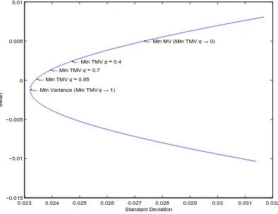
•← Min Variance (Min TMV q → 1) •← Min TMV q = 0.7
•← Min TMV q = 0.4
•← Min TMV q = 0.95
[image:20.595.99.493.231.534.2]•← Min MV (Min TMV q → 0)
Figure 2: Portfolio frontier showing optimal portfolios obtained by minimizing (i) variance (Min Variance),
(ii) tail mean-variance criterion (Min TMV) at different confidence levels q = 0.4,0.7,0.95, (iii)
mean-variance criterion in that an investor can account for his aversion to tail risk. As
demonstrated by Landsman (2010) and depicted in Figure 2, the ‘Min TMV’ portfolio tends
to the ‘Min MV’ portfolio as q → 0; on the other hand, it tends to the global minimum variance portfolio asq →1. An investor can specify theq-quantile of loss beyond which he
is sensitive to losses. The greater this threshold is, the more sensitive he is to large losses,
and the more conservative his optimal portfolio becomes.
6. Tail Mean-Variance Optimization with a Risk-Free Asset
Suppose that a risk-free asset earning a non-random rateris introduced to the portfolio
opportunity set. The overall portfolio of an investor then consists of holding a proportion,
say y∈ R, of total wealth in a sub-portfolio of risky securities and the remainder (1−y) in the risk-free asset. We assume that there is no constraint on the risk-free asset, i.e. that
both risk-free lending and borrowing at rate r are possible.
6.1. Classical Mean-Variance Optimization with Risk-Free Lending and Borrowing
We first consider classical mean-variance optimization only. It is well-known that the
efficient frontier of the overall portfolio, in mean-standard deviation space, is a straight line
with a positive slope and a vertical intercept at r. As emphasized by Merton (1972), three
cases can arise, depending on the level of the risk-free rate r relative to the mean return
of risky assets. The three cases depend, more specifically, on the relationship between the
risk-free rater and the mean return on the minimum variance portfolio x0. The first case
is economically significant and tends to be the only one dealt with in elementary texts
(Sharpe et al., 1995; Elton et al., 2011), but for completeness we consider all three possible
cases below.
Case 1. r < µTx0 ⇔ 1TΣ−1(µ−r1) > 0.
In mean-standard deviation space, the efficient frontier is a straight line with a positive
slope starting from the risk-free asset rf and going through a “tangency” portfolio xt:
xt =
Σ−1(
µ−r1)
1TΣ−1(
µ−r1)
See e.g. Kennedy (2010, p. 16). Note that xt ∈ E, where E is defined in equation (18) and
represents the original efficient frontier of risky securities only. In this case, xt is never
shorted, i.e. y ≥ 0. If y > 1, then the investor borrows at rate r; if y < 1, the investor lends at rate r; and if y= 1, there is neither lending nor borrowing.
Case 2. r > µTx0 ⇔ 1TΣ−1(µ−r1) < 0.
The efficient frontier is again a straight line with a positive slope from r, but this time
it consists of short positions in xt financing long positions in the risk-free asset. Thus,
y≤0.
Notice that the denominator of xt in equation (35) is negative in Case 2. In fact, xt
now lies in the lower half of the hyperbolic mean-variance frontier of risky securities only,
so the straight line efficient frontier isnot tangential toE in this case, but rather lies above it. For details, see Merton (1972) and Huang and Litzenberger (1988, p. 79).
Case 3. r = µTx0 ⇔ 1TΣ−1(µ−r1) = 0.
The efficient frontier is again a straight line with a positive slope from r, but now
consists of all wealth invested in the risk-free asset, along with investment, of a proportion
y ≥ 0 of wealth, in the self-financing portfolio z introduced in equation (17). While we
do not show this explicitly here, it is not difficult to show that the “arbitrage portfolio”
derived by Huang and Litzenberger (1988, p. 80) is identical to z.
6.2. Tail Mean-Variance Optimization with Risk-Free Lending and Borrowing
We now return to tail mean-variance optimization.
Theorem 2. Suppose that both risk-free lending and borrowing at rate r are available. (a) If r 6= µTx0, then the optimal tail mean-variance portfolio consists of holding a
proportion y∗
of wealth in tangency portfolio xt and the rest in the risk-free asset, where
y∗
=
A(B−λ1,q)
2λλ2,qB
if λ1,q ≤B
0 if λ1,q ≥B
and xt is given in equation (35). In the above, A=1TΣ−1(µ−r1) and
B =
q
(µ−r1)TΣ−1(µ−r1).
(b) If r = µTx0, then the optimal tail mean-variance portfolio consists of investing all
wealth in the risk-free asset and investing a proportion y∗
of wealth in the self-financing portfolio z, where
y∗
=
C−λ1,q
2λλ2,qC
if λ1,q ≤C
0 if λ1,q ≥C
(37)
and z is given in equation (17). In the above, C =pµTΣ−1(µ−r1).
Refer to Appendix A.2 for a proof of Theorem 2.
In the most common situation (described by case 1 in section 6.1), the risk-free rate is
lower than the average return on the global minimum variance portfolio of risky securities.
A situation where this did not hold would be unsustainable in the long term as it would
result in a flight from risky assets into short-term Treasury bills, depressing risky security
prices to the point where their expected return would rise relative to the risk-free rate.
Equation (36) in Theorem 2 is then seen to be a sensible proposition from a portfolio
management point of view. The more risk-averse a tail mean-variance-minimizing investor
is, the larger λ or λ1,q or λ2,q in equation (13) is likely to be, and therefore the more of
his wealth, in relative terms, he will invest in the risk-free asset and the lower y∗
is in
equation (36). If he is so risk-averse that λ1,q is greater than the threshold represented by
B, then he will invest only in the risk-free asset (y∗
= 0).
The fact that there is such a threshold is peculiar to the tail mean-variance criterion.
Indeed, there is no such threshold in classical mean-variance portfolio theory. To explain
this feature, we resort to a visual interpretation in µ–σ space, where µ is the mean and σ
is the standard deviation of portfolio returns. From equations (1) and (13),µ=λλ2,qσ2+
λ1,qσ−T M V and contours of equal tail mean-variance criterion are convex in µ–σ space.
Now, iso-TMV contours have a slope that is not less thanλ1,q, sincedµ/dσ= 2λλ2,qσ+
λ1,q. In fact, at their point of intersection with the vertical axis (σ = 0), they have a slope
of λ1,q. On the other hand, the straight line mean-variance efficient frontier, joining the
risk-free asset r to the tangency portfolio xt, has a slope of (µTxt −r)/
√
xtTΣxt = B
(in case 1). Consequently, when λ1,q > B, the iso-TMV contours are always steeper than
the straight line efficient frontier, so that no point of tangency occurs. The portfolio that
yields the lowest TMV occurs at the point where the highest iso-TMV contour intersects the efficient frontier, and is therefore the risk-free asset (y∗
= 0). The lowerλ1,q is, the less
steep the contours of level TMV are; the tangency point between iso-TMV contours and efficient frontier then moves higher up along the straight line efficient frontier.
This is in sharp contrast to classical mean-variance optimization with theMV criterion (g(x)) in equation (14), where there is always a tangency point between contours of equal
MV and the straight line efficient frontier (at least for investors who are not perfectly risk-averse and for whom τ < ∞ in equation (14)). These contours are also convex but
have a slope of zero when σ = 0, compared to a positive slope ofλ1,q in the TMV case. In
a loose sense, one might state that theTMV criterion generally implies a higher degree of risk aversion than the MV criterion.
Part (b) of Theorem 2 is also deserving of comment. This refers to the unusual case
where the risk-free rate coincides exactly with the mean return on the minimum variance
portfolio (case 3 in section 6.1), whereupon no tangency portfolio exists. This result was
first derived by Merton (1972) in the classical mean-variance context. The efficient frontier
of risky securities only, defined as E in equation (18), has an asymptote that goes through
the risk-free asset and has a slope of C (Huang and Litzenberger, 1988, p. 79). In the
classical mean-variance case, optimal portfolios then lie on this asymptote, and consist
of all wealth being lent risk-free, together with a self-financing investment in portfolio z
requiring no additional wealth. Again, if a TMV-minimizing investor is sufficiently risk-averse, the slope of his contours of level TMV will be high enough that they are never tangential to the asymptote, so that investment inz does not occur (y∗
7. Conclusion
Asset return distributions are known to be heavy-tailed. Investors are also sensitive
to extreme events in the capital and insurance markets, which occur in the tail of return
distributions. The tail mean-variance criterion, which is considered in this paper, enables
investors to select portfolios that take into account the risk of large but rare losses. It
uses both the tail conditional expectation and the tail variance risk measures. If returns or
losses are jointly elliptically distributed, then an analytic solution for the optimal portfolio
under the tail mean-variance criterion is available. We characterized this optimal portfolio
as a mean-variance efficient portfolio, even though the tail mean-variance criterion is not
a translation-invariant positive-homogeneous risk measure. We also derived an explicit
solution for the optimal portfolio, which improves on previous work by providing both
insight and computational convenience, avoiding the partition, inversion and concatenation
of large matrices. In the presence of a risk-free asset, the optimal portfolio remains
mean-variance efficient. For a range of parameter values in the tail mean-mean-variance criterion that
imply greater aversion to losses beyond a certain threshold, it turns out to be optimal to
invest only in the risk-free asset. The optimal portfolios that we calculated are simple
enough that risk managers and portfolio managers can readily compute and implement
them.
Appendix A. Proofs
Appendix A.1. Proof of Lemma 4
F(0) > 0 and F(a) < 0 and F(x) → +∞ as x → ±∞, hence F(x) has at least one
real zero in (0, a) and at least one real zero in (a,∞). Denote these two zeros by x1 and x2 respectively. There are two possible cases concerning the remaining two zeros, say x3
and x4.
First, x3 and x4 may be complex conjugates, in which case x1 and x2 are indeed
coincident withx1 or x2.
F(x) = x4
−2x3 + (a2
+b−c)x2
−2bx+a2
b. (A.1)
The coefficient ofx3 in the above is negative
⇒P
xi <0. Therefore, at least one ofx3 and
x4 is negative. Further, the coefficient of x is also negative ⇒ F′
(0)<0. Since F(0) >0,
it follows that both of x3 and x4 are negative (possibly coincident). Hence, x1 and x2 are
non-repeated real zeros.
This completes the proof of Lemma 4.
As an aside, we note that a2+b
−c < 0⇒ x1 ∈(0, a),x2 ∈(a,∞), andx3 and x4 are complex conjugate roots, by virtue of Descartes’ rule of signs applied to the coefficients of
F(x) in equation (A.1). In fact, were the sign of a2 +b
−c to be specified, then Sturm’s theorem (Itˆo, 1993, p. 36) would be applicable.
Appendix A.2. Proof of Theorem 2
Let µ be the mean return on an overall portfolio (of risky and risk-free assets) and σ
be the standard deviation of return on this overall portfolio. Then the tail mean-variance
criterion may be written as
f(x) = −µ+λ1,qσ+λλ2,qσ2. (A.2)
Note that the proportion invested in the risk-free asset is 1−y= 1−1Tx.
By an argument similar to the proof of Lemma 3, the portfolio that minimizes the tail
mean-variance criterion in equation (A.2) must lie on the straight line efficient frontier:
denote the mean return on the tail mean-variance optimal portfolio by µ∗
, its standard
deviation byσ∗
, and the minimal value of the criterion byϕ∗
; suppose that the tail
mean-variance optimal portfolio does not lie on the efficient frontier; then there exists an overall
portfolio, with mean returnµ1 and standard deviation σ1 and tail mean-variance criterion
ϕ1, that satisfies µ1 ≥ µ∗
and σ1 < σ∗
; but, by equation (A.2), this would imply that
ϕ1 < ϕ∗
The tail mean-variance optimal portfolio is therefore a mean-variance efficient portfolio
belonging to one of the three cases described in section 6.1. Given sgn(µTx0 −r), the
optimal portfolio is fully specified byy.
Case 1. y ≥ 0 and A > 0. Define µt to be the mean return on the tangency portfolio xt
and σt to be its standard deviation of return. The mean return on an efficient portfolio
in case 1 is µ= yµt+ (1−y)r and the standard deviation of its return is σ = yσt, with
y ≥ 0. The tail mean-variance criterion of equation (A.2) is therefore f(y) = −r−(µt−
r)y+λ1,qσty+λλ2,qσt2y
2 and has at most one minimum, since f′′
(y) = 2λλ2,qσt2 >0.
From the tangency portfolio xt in equation (35), it is straightforward to find that
µt =C2/A and µt−r =B2/A and σt2 =B
2/A2. Furthermore, σ
t =B/|A|= B/A, since
A > 0 in case 1. Note that B2 = (
µ−r1)TΣ−1(µ−r1) > 0 and B ∈ R++ by virtue of positive definiteness of Σ (and hence of Σ−1), and by the assumption of linear independence
of µ and 1. Therefore, f(y) = −r−(B2/A)y+λ1,q(B/A)y+λλ2,q(B/A)2y2
The Kuhn-Tucker conditions are y≥0, f′
(y)≥0 and yf′
(y) = 0. The complementary
slackness condition is satisfied either by f′
(y∗
) = 0 ⇔ y∗
= A(B −λ1,q)/2λλ2,qB, with
y∗
≥0 provided that λ1,q ≤B; or byy∗ = 0, in which case f′(0)≥0 provided λ1,q ≥B.
Case 2. y ≤ 0 and A < 0. Constrained minimization proceeds as in case 1 above. The standard deviation of return on the tangency portfolio is now σt = B/|A| = −B/A,
since A < 0 in case 2. But the standard deviation of return on the overall portfolio is
σ =−yσt =yB/A (sincey ≤0). Therefore,f(y) is unchanged from case 1.
The Kuhn-Tucker conditions do change because of the non-positivity constraint: they
are y ≤ 0, f′
(y) ≤ 0 and yf′
(y) = 0, and are satisfied either by f′
(y∗
) = 0 ⇔ y∗
=
A(B −λ1,q)/2λλ2,qB, with y∗ ≤ 0 provided that λ1,q ≤ B; or by y∗ = 0, in which case
f′
(0)≤0 provided λ1,q ≥B. (Recall that A <0 in case 2.)
y∗
for cases 1 and 2 may therefore be combined in equation (36), which captures both
long and short positions in the tangency portfolio.
Define µz to be the mean return on portfolio z and σz to be its standard deviation of
return. Substituting r=µTx0 into equation (22) gives µz =µTΣ−1(µ−r1) =C2. From
equation (24), σ2
z = µz = C2. Note that C2 = µTΣ−1(µ−r1) > 0 and C ∈ R++ since µz = σ2z > 0. This is also confirmed by an application of the Cauchy-Schwarz inequality
to the term in square brackets on the r.h.s. of equation (24).
The mean return on an efficient portfolio in case 3 is therefore µ=r+µzy =r+C2z,
and the standard deviation of its return is σ =yσt =yC, with y≥0 and C > 0. The tail
mean-variance criterion of equation (A.2) is thereforef(y) = −r−C2y+λ1
,qCy+λλ2,qC2y2
and has at most one minimum, since f′′
(y) = 2λλ2,qC2 >0.
The Kuhn-Tucker conditions for a minimum inf(y) wrtysubject to the non-negativity
constraint on y lead again to two possible solutions: either f′
(y∗
) = 0 ⇔ y∗
= (C − λ1,q)/2λλ2,qC which is non-negative provided λ1,q ≤C; ory∗ = 0 with f′(0)≥0 provided
that λ1,q ≥C.
This completes the proof of Theorem 2.
References
Acerbi, C., Tasche, D., 2002. On the coherence of expected shortfall. Journal of Banking
and Finance 26(7), 1487–1503.
Artzner, P., Delbaen, F., Eber, J.M., Heath, D., 1999. Coherent measures of risk.
Mathe-matical Finance 9, 203–228.
Chacko, G., Viceira, L.M., 2005. Dynamic consumption and portfolio choice with stochastic
volatility in incomplete markets. Review of Financial Studies 18(4), 1369–1402.
Chiragiev, A. and Landsman, Z., 2007. Multivariate Pareto portfolios: TCE-based capital
allocation and divided differences. Scandinavian Actuarial Journal 4, 261–280.
Elton, E.J., Gruber, M.J., Brown, S.J., Goetzmann, W.N., 2011. Modern Portfolio Theory
Fang, K.T., Kotz, S., Ng, K.W., 1990. Symmetric Multivariate and Related Distributions.
Chapman and Hall, London.
Furman, E., Landsman, Z., 2005. Risk capital decomposition for a multivariate dependent
gamma portfolio. Insurance: Mathematics and Economics 37(3), 635–649.
Furman, E., Landsman, Z., 2006. Tail variance premium with applications for elliptical
portfolio. ASTIN Bulletin 36(2), 433–462.
Garlappi, L., Uppal, R., Wang, T. 2007. Portfolio selection with parameter and model
uncertainty: A multi-prior approach. Review of Financial Studies 20(1), 41–81.
Huang, C., Litzenberger, R.H., 1988. Foundations for Financial Economics. Prentice Hall,
Englewood Cliffs, New Jersey.
Itˆo, K. (ed.), 1993. Encyclopedic Dictionary of Mathematics, 2nd ed. MIT Press,
Mas-sachusetts.
Jorion, P., 1996. Risk2
: Measuring the risk in Value at Risk. Financial Analysts Journal
52(6), 47–56.
Kan, R., Zhou, G., 2007. Optimal Portfolio Choice with Parameter Uncertainty. Journal
Of Financial And Quantitative Analysis 42(3), 621-656.
Karatzas, I., Shreve, S.E., 1991. Brownian Motion and Stochastic Calculus. Springer,
Berlin.
Kennedy, D., 2010. Stochastic Financial Models. Chapman and Hall/CRC Press, Boca
Raton, Florida.
Landsman, Z.M., 2010. On the Tail Mean-Variance optimal portfolio selection. Insurance:
Mathematics and Economics 46, 547–553.
Landsman, Z.M., Valdez, E.A., 2003. Tail conditional expectations for elliptical
Landsman, Z.M., Valdez, E.A., 2005. Tail conditional expectations for exponential
disper-sion models. ASTIN Bulletin 35(1), 189–209.
Lee, C.-F., Lee, C. (ed.), 2006. Encyclopedia of Finance. Springer.
Markowitz, H.M., 1952. Portfolio selection. Journal of Finance 7, 77–91.
McNeil, A.J., Frey, R., Embrechts, P., 2005. Quantitative Risk Management. Princeton
University Press.
Merton, R.C., 1969. Lifetime portfolio selection under uncertainty: the continuous-time
case. Review of Economics and Statistics 51, 247-257.
Merton, R.C., 1971. Optimum consumption and portfolio rules in a continuous-time model.
Journal of Economic Theory 3, 373-413.
Merton, R.C., 1972. An analytic derivation of the efficient portfolio frontier. Journal of
Financial and Quantitative Analysis 7(4), 1851–1872.
Neumark, S., 1965. Solution of Cubic and Quartic Equations. Pergamon Press, Oxford.
Owen, J., Rabinovitch, R., 1983. On the class of elliptical distributions and their
applica-tions to the theory of portfolio choice. Journal of Finance 38(3), 745–752.
Panjer, H.H., 2002. Measurement of risk, solvency requirements, and allocation of capital
within financial conglomerates. University of Waterloo, Canada.
Panjer, H.H. et al., 1998. Financial Economics. The Actuarial Foundation, Schaumburg,
Illinois.
Sharpe, W.F., Alexander, G.J, Bailey, J.V., 1995. Investments, 5th ed. Prentice Hall,
Englewood Cliffs, New Jersey.
Tu, J., Zhou, G., 2004. Data-generating process uncertainty: what difference does it make
Yang, H., Zhang, L., 2005. Optimal investment for insurer with jump-diffusion risk process.
Insurance: Mathematics and Economics 37, 615-634.
Zhao, H., Rong, X., 2012. Portfolio selection problem with multiple risky assets under
the constant elasticity of variance model. Insurance: Mathematics and Economics 50(1),