City, University of London Institutional Repository
Citation
:
Kandler, A. and Laland, K. N. (2013). Tradeoffs between the strength of conformity and number of conformists in variable environments. Journal of Theoretical Biology, 332, pp. 191-202. doi: 10.1016/j.jtbi.2013.04.023This is the accepted version of the paper.
This version of the publication may differ from the final published
version.
Permanent repository link:
http://openaccess.city.ac.uk/7622/Link to published version
:
http://dx.doi.org/10.1016/j.jtbi.2013.04.023Copyright and reuse:
City Research Online aims to make research
outputs of City, University of London available to a wider audience.
Copyright and Moral Rights remain with the author(s) and/or copyright
holders. URLs from City Research Online may be freely distributed and
linked to.
Tradeoffs between the strength of conformity and number of
conformists in variable environments
Anne Kandler1,2,* 1
Department of Mathematical Science, City University London, Northampton Square, London EC1V 0HB, UK 2
Santa Fe Institute, 1399 Hyde Park Road, 87501 Santa Fe (NM), USA *Corresponding author
Email: [email protected]
Phone: (+44) 020 7040 8464 Fax: (+44) 020 7040 8568
Kevin N. Laland3 3
School of Biology, St. Andrews University, Bute Building, Queens Terrace, St. Andrews, Fife KY16 9TS, UK
Abstract. Organisms often respond to environmental change phenotypically, through learning strategies that enhance fitness in variable and changing conditions. But which strategies should we expect in population exposed to those conditions? We address this question by developing a mathematical model that specifies the consequences of different mixtures of individual and social learning strategies on the frequencies of different cultural variants in temporally and spatially changing environments. Assuming that alternative cultural variants are differently well-adapted to diverse environmental conditions, we are able to evaluate which mixture of learning strategies maximizes the mean fitness of the population. We find that, even in rapidly changing environments, a high proportion of the population will always engage in social learning. In those environments, the highest adaptation levels are achieved through relatively high fractions of individual learning and a strong conformist bias. We establish a negative relationship between the proportion of the population learning socially and the strength of conformity operating in a population: strong conformity requires fewer conformists (i.e. larger proportion of individual learning), while many conformists can only be found when conformist transmission is weak. Investigations of cultural diversity show that in frequently changing environments high levels of adaptation require high level of cultural diversity. Finally, we demonstrate how the developed mathematical framework can be applied to time series of usage or occurrence data of cultural traits. Using Approximate Bayesian Computation we are able to infer information about the underlying learning processes that could have produced observed patterns of variation in the dataset.
Keywords: Social learning, conformity, environmental heterogeneity, diffusion-reaction systems, cultural diversity, Approximate Bayesian Computation
1 Introduction
environmental conditions frequently face the task of choosing between cultural variants according to their apparent utility. That they are able to do so effectively is illustrated by the observation that human
behavioural ecologists can predict human behaviour by assuming individuals to be well-adapted to their environment [6,7].
Broadly speaking, an individual’s choice between alternative cultural variants can be guided by different individual and social learning strategies. While social learning refers to learning that is influenced by observation of or interaction with other individuals or its products individual learning refers to learning (e.g. trial and error) that does not involve social interactions or any information provided by others [15]. Given the fact that social human learning is rule governed, with many possible rules [4,20,24], we can ask which learning strategy, or strategies, should be expected in populations living in temporally and spatially changing environments (where ‘environments’ encompass social, ecological and physical variables).
Formal population-genetic and game-theory analyses have explored this question by determining the evolutionary stable strategies, and thereby identifying the strategies that would evolve under natural selection. It has been suggested that individual and social learning are favoured by natural selection when temporal environmental changes occur at relatively short and long intervals, respectively (e.g.
[1,4,5,11,31]). Boyd and Richerson [4,5] developed a series of mathematical models to understand the conditions under which individual and social learning are adaptive. In their models, individual learning allows an individual to acquire behaviour that is adaptive to the local environments by evaluating
environmental cues. This process may, depending on the quality of these cues, lead to errors. However, if environmental cues are ambiguous, individuals may benefit from copying the behaviour of another individual from the previous generation. The challenge the individuals face is to match the correct
behaviour to the current environmental conditions. Boyd and Richerson [5] concluded that heavy reliance on social learning is most adaptive if individual learning is inaccurate (or costly to make accurate). Further, when the environment does not change too quickly, and there is not too much migration among habitats, the “occasional use of independently acquired compelling evidence coupled with faithful copying in the absence of such evidence is sufficient to keep the locally adaptive behaviour common” [5, page 43]. Rogers [31] developed a somewhat similar model, but assumed that an individual either learns individually or socially, with individual learning occurring without error. He concluded that the population is expected to reach an equilibrium at which individual and social learners will be equal in their fitness. Rendell et al. [28] however showed that by adding a spatial structure to this problem the mixed equilibrium may not occur.
Feldman et al. [11] generalised those models by allowing for genetic evolution through the use of a gene-culture coevolutionary model, where the decision to learn individually or socially is determined by a fixed genotype-dependent probability. They found that both fixation of individual learning and the stable coexistence of individual and social learning are possible in changing environments. Like Boyd and
Richerson [5], they concluded that the greater the probability of environmental change the more difficult is it for social learning to evolve (see also [1,36]). Aoki and Nakahashi [2] analysed the evolution of social learning in spatial heterogeneous environments under different migration rates. They found that increased migration hinders social learning and pointed to the importance of population structure on the evolution of social learning. In contrast, the simulation approach of the ‘social learning strategies tournament’
tournament), which allows social learners to adjust their behaviour flexibly following environmental change, switching between the variants in their repertoire to maintain adaptive behaviour.
There is further ambiguity over the most effective means of social learning - that is, which ‘social learning strategy’ (or ‘transmission bias’) to deploy - under variable environmental conditions. Henrich and Boyd [14] studied the evolution of conformity, a frequency-dependent transmission bias promoting the disproportional adoption of common behaviour. They developed a two-locus haploid asexual model where one locus determines the reliance on social learning as opposed to individual learning and the second locus determine the strength of the conformist effect. Their model suggested that selection favours conformist transmission as long as the environment does not change too rapidly and the evolution of social learning is more strongly influenced by environmental heterogeneity than the evolution of conformity. They also found that increased migration impeded social learning but has little effect on the evolution of conformity.
Nakahashi [26], Wakano and Aoki [35] and Kendal et al. [19] all challenged aspects of Henrich and Boyd’s findings, by reporting a negative relationship between the stability of the environment and the reliance on conformist bias. The reliance on conformity tends to be larger when the cycle of environmental change is shorter (i.e. for rapid change). The Henrich and Boyd model differs from these other models [19,26,35] in a number of respects, including the manner in which individuals use asocial and social information. While Henrich and Boyd [14] assume mixed strategies, Nakahashi [26], Wakano and Aoki [35] and Kendal et al. [19] all assume pure strategies where individuals use either social or individual learning to update their behaviour. Eriksson et al. [10] criticised Henrich and Boyd’s assumptions, arguing that it is unrealistic to assume that individuals know all variants at any time or that only two cultural variants exist in the population. On the base of their model, Eriksson et al [10] concluded that a relaxation of either of these assumptions is disadvantageous to the evolution of a conformist strategy. Efferson et al. [9] found that the evolutionary advantage of conformity depends on the accuracy of individual learning.
However, McElreath et al. [24] claim that neglecting spatial heterogeneity, as occurs in the models of Nakahashi [26], Wakano and Aoki [35], Kendal et al. [19] and Eriksson et al. [10], may diminish the effectiveness of conformity.This suggestion is plausible, since spatial variation promotes reliance on conformity [4]. Similarly, Nakahashi et al. [27] argue that focusing on situations with (i) only two cultural variants present, (ii) temporally varying environments and (iii) error-free cultural transmission has obscured conditions favouring the evolution of conformity.
In summary, efforts to explore the relationship between environmental uncertainty and learning strategies have mainly focused on analyzing evolutionary stable equilibria and it is understood that
easily. Therefore the analysis of temporal and spatial patterning of those usage and occurrence frequencies might provide an alternative way of investigating which learning strategies are employed by a population.
We explore this approach by developing a mathematical model, which tracks the spatial and temporal frequency distributions of different cultural variants in different environmental and cultural conditions. We base our model on the assumption that frequency changes of cultural variants are mainly attributed to individual and social learning strategies and therefore establish a causal relationship between changes in frequency and learning strategies employed by the population. Further, we assume that the considered cultural variants confer different levels of benefit in different environmental settings (as expressed by the variant’s ‘adaptation functions’) and that the strength with which learning strategies favour one variant over another is dependent on the conferred benefit. This framework enables us to explore the effects of different learning strategies on the frequency distribution of cultural variants over time and space in changing environments and consequently to quantify the adaptation level of the population with respect to the considered cultural trait. In this way we can infer which learning strategies should be expected in populations showing low and high levels of adaptation, respectively and can explore which learning strategy leads to the highest adaptation level of the population, hence fitness, given a certain level of environmental uncertainty. Our interpretations assume that sufficient time has passed for the optimum to be reached and that selection will typically favour traits that maximize average fitness [23]. Additionally the framework allows us to investigate the effects of individual and social learning on cultural diversity. Here, we build on our earlier analyses [17], which explored the relationship between the rate of innovation and level of cultural diversity in homogeneous environments.
In contrast to previous research, our approach assumes temporally fixed learning strategies and consequently we cannot draw any conclusion about the evolutionary stability of strategies leading to high levels of adaptation as natural selection does not always favour strategies maximizing average adaptation levels (e.g. [12,16]). In constant environments it has been shown (e.g. [8,21]) that, subject to consistent selection, evolutionary stable strategies maximize the adaptation level of well-mixed populations, but under frequency-dependent selection stable equilibria usually result in adaptation levels lower than the maximum. Therefore subsequent analyses to those presented here will be required to establish whether the identified strategies leading to the highest average adaptation level are evolutionary stable. However, the strategies which maximize average fitness often provide a good first indication what is likely to develop especially when the considered system exhibits some stochasticity. Further, using the strategies identified by previous research as model input will allows us to analyse the expected frequency changes of different cultural variants under those strategies and consequently to compare these change pattern to available data.
2 The model
The central element of our model is a cultural trait, which is represented by different variants serving a similar function but differing in the benefit conferred in different environmental conditions. The variants are adopted by individuals of a single population, distributed across a two-dimensional domain
D=[0,1]x[0,1].Individuals choose between alternative variants according to the adoption mechanisms specified below. The population experiences temporally and spatially changing environment conditions, expressed by the function e(t,x), , with ( ) . Changing environmental conditions affect the adaptation levels of the different cultural variants and we characterize each variant i
by its ‘adaptation function’, or ai(e(t,x)). The adaptation function quantifies the fitness level that variant i
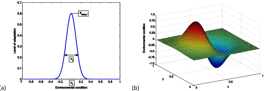
conveys to its adopter in environmental state e(t,x). Fitness levels vary in the interval [0,1] with 0 indicating no fitness and 1 describing the situation of optimal adaptation. Figure 1a gives an example of such an adaptation function; ai(e) is zero if the use of variant i provides no advantage to the adopter in environment
e and has a positive value otherwise. We assume aito be a bell-shaped function, which possesses its
maximum value amax,i, where in our analyses 0.2≤amax,i ≤1, at the environmental state µi to which the variant
is best adapted. The width of the function ai is determined by the parameter σi, where in our simulations
0<σi≤0.06, which can be interpreted as a measure of the generality of the specific variant (The larger σithe
larger is the environmental range over which the variant provides a benefit to its adopters)1. Hence each cultural variant is determined by the parameter set (µi, σi,amax,i). We begin each simulation run by
generating a pool of 15 variants, choosing their parameters µi, σiand amax,i randomly within the assumed
ranges. We restrict ourselves to 15 variants in order to make the computational effort manageable, however test runs with more than 15 variants showed that the results do not change qualitatively.
(a) (b)
Figure 1. (a) Example of an adaptation function ai, (b) Our spatial heterogeneous environment.
The randomly chosen variants are introduced into the population at random locations (although variants are only introduced into areas where they provide some sort of benefit at the time of invention, meaning where ai(e(0,x))>0.05 holds). Given our assumption that all cultural variants fulfil a similar function, they can
be considered as competing with each other for use. This competition is manifested in the manner in which
1
We assume the parameters amax,i and σi are correlated in order to account for the fact that more general applicable
[image:6.612.80.535.423.580.2]the population adopts the different variants. We distinguish between two main adoption mechanisms, (i) social learning, in the form of both directly biased transmission and frequency-dependent transmission and (ii) individual (or asocial) learning. We note, that in reality, human social learning strategies are likely to be more complex than those considered here (e.g. [25, 38]).
Individual and social learning differ in the kind of information used to form the adoption decision. Here individual learning is based on judgments about the utility of specific variants in observed
environmental conditions. This process has two main error sources: misjudgement of the current
environmental condition e and misjudgement of the adaptation level conferred by the different variants. Although these error sources are conceptually different, they lead to the same outcome in our modelling framework: a variant k is chosen for which µk≠e. Therefore we model the inaccuracy of individual learning
by assuming that individual learning is based on an environment ̅( ) ( ) with , where the variance models the reliability of individual learning. Unless otherwise indicated, we assume . Despite being error-prone, individual learning can introduce new variants in a specific area of the domain.
In contrast, social learning can act only on variants that already exist in a specific area, leaving social transmission frequency-dependent. In the following we explore the dynamics of two specific social learning mechanisms, directly biased transmission and frequency-dependent transmission, deploying the
formulation of Henrich [13]. Further, we assume that the transmission processes occur accurately. Directly biased transmission is defined as the selective copying of pre-existing variants found to be efficacious by individual assessment [4] and is characterised by a positive correlation between the adaptation level of the variant and the strength of social learning. (This rule is sometimes referred to as ‘payoff-based copying’ [19,20,25,38]). Using this strategy, the naive members of the population (individuals who have not yet adopted a cultural variant) would adopt variant i at a rate ri=ri(ai) with ai=ai(e(t,x)), where in our simulations
0≤ri≤0.15. This rate ri can be interpreted as the mean judgment, across the population, of the benefit this
variant might convey, and we assume that the higher the adaptation level ai(e(t,x)), the higher the adoption
rate ri. Further, individuals who already possess a variant might consider switching to another variant if it
provides a greater benefit. We define the rate at which individuals who have adopted variant i switch to variant j as cij=cij(ai(t,x),aj(t,x)), where in our analyses 0≤cij≤0.08. We assume that the rate cij depends on the
difference in the adaptation levels of the variants: the higher the difference aj(e(t,x))-ai(e(t,x)) the more
likely individuals are to switch.
Frequency-dependent transmission neglects fitness information and leads to a disproportional adoption of variants whose frequencies fall above or below a commonness threshold cB[4]. Here, this
frequency-dependent bias is modelled by(1-b)ri+b(ui-cbK(t)) and [(1-b)cij+b(uj-cbK(t))]+where ui and uj
describe the frequencies of variants i and j, K stands for the population size at time t and the coefficient b
determines the strength of the frequency-dependent bias by quantifying the respective importance of fitness and frequency information on the adoption decision. For b>0 we obtain a conformist transmission bias: the more a variant’s frequency exceeds the threshold cb the stronger the variant is supported by the
bias.
All cultural adoption rules specified above act locally in location x. However, spatial interactions are ensured by the dispersal behaviour of the population, with individuals carrying variants into new locations. Spatial dispersal is defined by the diffusion components diΔuiwhich describes the spread of the variants
based on a random walk assumption. The scale of spatial interactions within the population is given by the diffusivity2di. Unless otherwise specified, in our analyses d=10-4. The diffusion approach implies that the
direction of dispersal is uncorrelated with the locations of the environmental conditions in which the variants, carried by the individuals, are beneficial.
In order to model temporal and spatial environmental changes we define a parameter ε (denoted as environmental instability), which describes the fraction of the environment that is changed in every time step. We discretize the two-dimensional domain D into a lattice {lrs}r,s=1,…,m where 1/m describes the
discretization length in both spatial directions and add to ε percent of the lattice points a random variable . Unless otherwise indicated we set . In order to avoid changes that occur suddenly in time and space, we smooth the environment in temporal and spatial direction and obtain a continuous differentiable two-dimensional surface e(t,x), . Our model of environmental change allows for the recurrence of conditions especially as we restrict the range of possible environmental
conditions to E=[-1,1].
With ξ and η=1-ξ describing the fractions of the population relying on individual and social learning, respectively we formulate the described dynamics in a spatial and temporal explicit n-variant diffusion-reaction competition framework that models the changes of the variant’s frequencies ui over time and
space. We solve the system of differential equation using the Finite-Element Method (FEM) (e.g. [37]). This method is a numerical technique for finding approximate solutions to systems of partial differential
equations where the geometrical domain of the considered problem is discretized using sub-domain elements, called the finite elements, and the differential equations are applied to a single element after they are transformed to an integro-differential formulation. Based on such FEM solutions ui(t,x), which
describe the spatial frequency distribution of variant i at time t, and the level of adaptation ai(e(t,x)) of the
different variants, we are able to determine the level of adaptation of the population to the experienced environmental conditions at every time t and location x
̅ ( ) ∑ ( ( )) ( )
and the overall level of adaptation
( ) ∑ ∑ ( ( )) ( ),
where n describes the number of variants present in the population. For convenience we average over the adaptation level at the grid points of the lattice {lrs}r,s=1,…,m, which discretizes the considered domain D.
Based on these variables we quantify the effects of different fractions of the population relying on
individual and social learning on the adaptation situation under different levels of environmental instability. All results described below are obtained by averaging over 10,000 solutions of the diffusion-reaction framework. We stress that our approach does not deal with the consequences of the adoption decisions of a single individual, but rather with the cumulative consequences of the decisions of all individuals in the population on the frequencies of the different cultural variants. A full description of the mathematical model can be found in Appendix A.
2
Diffusivity is measured in the dimension [length]2/[time] and is indicative of the speed of diffusion. For example the expression √ can be interpreted as the average distance covered in the time interval [0,t]. The value d=10-4 is chosen so that spatial interactions contribute to but not dominate the cultural dynamic.
~N(0,change2 )
change
3 Results
In this section we use the model to explore the relationship between environmental uncertainty, different learning strategies and the population’s level of adaptation and cultural diversity. We start by analysing the adoption dynamics of a population in a spatially heterogeneous but temporally constant environment as shown in Figure 1b. (Here we do not include individual learning but note that this does not change the adaptation dynamic qualitatively). We then go on to analyse the adoption dynamic in spatially and temporally heterogeneous environments.
3.1 Spatial heterogeneous environments
As described above, the 15 randomly chosen variants are introduced into the population at random locations (although variants are only introduced into areas where they provide some sort of benefit, where
ai(e(0,x))>0.05 holds); the dispersal behaviour of the population is responsible for their subsequent
diffusion over the considered domain D. Naturally, we find that the areas where variants prove to be well-adapted are larger in regions with relatively little spatial variability, causing those variants to be present at high frequencies over larger regions. In contrast in more spatially variable environments, beneficial variants only raise the adaptation level of a smaller region. Furthermore, we find that the presence of a conformist bias typically leads to higher level of adaptation over time, with a sharper spatial distinction between the variants. In temporally constant environments, highly beneficial variants are likely to show high
frequencies, which then are reinforced by the frequency-dependent bias.
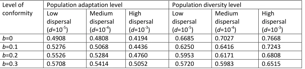
Dispersal facilitates the spatial spread of the different variants and therefore enhances the fitness of the population in the short term. However, as soon as variants became present in areas where they are well-adapted, dispersal can have the opposite effect: it can bring variants into areas where they might not be the best response to the environmental conditions while, depending on the difference between the levels of adaptation of variants, the switching process might not happen immediately. Table 1 gives the overall adaptation level apop of the population after 500 time steps, for different dispersal rates and
different levels of conformity.
Level of conformity
Population adaptation level Population diversity level Low
dispersal (d=10-5)
Medium dispersal (d=10-4)
High dispersal (d=10-3)
Low dispersal (d=10-5)
Medium dispersal (d=10-4)
High dispersal (d=10-3)
b=0 0.4908 0.4808 0.4194 0.6685 0.7027 0.7668
b=0.1 0.5276 0.5068 0.4436 0.6250 0.6416 0.7243
b=0.2 0.5526 0.5284 0.4760 0.5953 0.6171 0.6808
[image:9.612.61.558.504.617.2]b=0.3 0.5708 0.5414 0.5052 0.5720 0.5983 0.6515
Table 1. Population adaptation levels, population diversity indices for different levels of conformity and dispersal rates.
We also observe a positive relationship between the level of conformity necessary to maximize adaptation levels and the rate of dispersal: the higher the dispersal rates the higher the level of conformity needs to be in order to reach the higher adaptation level apop (cf. [4]). Conformity counteracts the effects of dispersal by
diffusion of the variants. Further, we note that the utility of conformity is time-dependent. The longer we allow the system to evolve the higher is the benefit of the conformist strategy.
Next we quantify the level of cultural diversity by calculating the average Shannon diversity index of the population defined by
( ) ∑ ∑ ( ) ( ),
where n describes the number of variants present. For convenience we average over diversity levels at the grid points of the lattice {lrs}r,s=1,…,m which discretizes the considered domain D. Table 1 shows the level of
cultural diversity, for the situations with and without conformity. The diversity-reducing property of conformist bias is apparent. The higher the value of b (the strength of the conformist bias) the lower is cultural diversity. As expected, dispersal increases diversity.
3.2 Spatially and temporally heterogeneous environments
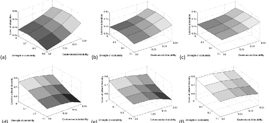
We now allow for both spatial and temporal changes in environmental conditions. As described above, it is a widely held view that, in temporally changing environments, social learning alone is not able to ensure an efficient and successful adaptation process to changed environmental conditions, since effective adaptation often requires a source of new variants (unless copy error introduces variation [29]). We find that a small amount of individual learning can fulfil this role and start our analysis by exploring the relationship between environmental instability ε (with ε describing the fraction of the environment that is changed in every time step), the population’s reliance on individual learning ξ and conformity b. Figure 2a-c show the overall adaptation level apop of the population after 500 time steps,
for different values of ε, ξ and b ((a): ξ=0.05, (b): ξ=0.1, (c): ξ=0.3).
(a) (b) (c)
[image:10.612.89.525.429.629.2](d) (e) (f)
Figure 2. Top row: Overall adaptation level apop of the population after 500 time steps for different fractions of the
population relying on individual learning ((a): ξ=0.05, (b): ξ=0.1, (c): ξ=0.3), levels of environmental instability
Individual learning can introduce new variants into a region and therefore can lead to a more successful adaptation process in temporally changing environmental conditions (cf. Figure 2a-c, across the
parameter range illustrated, an increase of the fraction of the population relying on individual learning leads to an increase in the overall adaptation level apop). However, this relationship does not hold
unboundedly. Due to the assumed error-prone nature of individual learning there exist a maximal value of ξ that can lead to the highest adaptation level of the population, for given values of ε and b.
Interestingly, even though social learning is often thought to be ineffective in unstable environments as variants present in the last time step might have no utility in the now changed environments (e.g. [11,14,33]) Figure 3b shows that the highest adaptation levels are reached with fractions of cultural social learning η never below 55%. Populations that show those high levels of adaptation in frequently changing environments are characterized by high levels of cultural diversity which are caused by high average numbers of present variants covering a broad range of possible conditions (cf. Figure 4). Consequently, social learning does not necessarily convey outdated information in changing environments if we allow for the accumulation of variants and therefore for cultural diversity in the population (a conclusion consistent with [30]). In this sense individual learning provides a set of variants from which social learning can choose. In the following we explore in detail how the adaptation process is affected by the different social learning strategies, cultural diversity, spatial dispersal, and the
accuracy of individual learning.
3.2.1 Effects of conformity
The effect of conformity on the overall adaptation level apop depends crucially on environmental
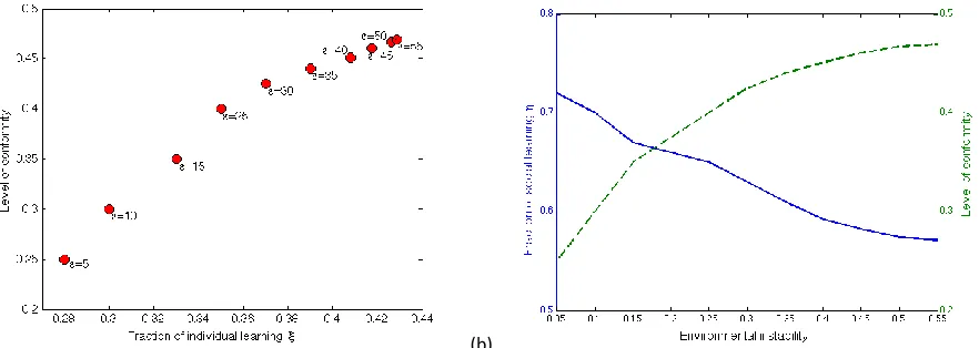
instability and the fraction of the population relying on individual learning. Figure 3a shows that (for given values of ε) there exist a pair of parameter values (bmax, ξmax=1-ηmax) leading to the highest level of
adaptation of the population. The more variable the environment the higher the fraction of individual learning and the strength of conformity need to be in order to maximize adaptation levels (cf. also [19,26,35]). Another way of thinking about this is to suggest that in less variable environments there is only a certain level of conformity that can be maintained, such that we witness a negative relationship between the strength of conformity and the proportion of the population learning socially, and hence deploying the conformist bias (cf. Figure 3b). This fact results from the opposing effects of conformity and individual learning on low-frequent variants. While individual learning introduces new variants usually at low frequencies into a region, conformist bias suppresses the spread of those variants. Now if the fraction of individual learning in the population is low then new variants are introduced only at very low frequencies and a medium or strong conformist bias can prevent those variants from spreading, even when they are well-adapted to the current environment. This hindrance slows down or even prevents the adaptation process and results in a lower overall adaptation level of the population. Therefore, in populations where only a small fraction of individuals rely on individual learning and which experience unstable environments, we expect at most very low levels of conformity (i.e. small b). However, if the fraction of individual learning becomes larger (and consequently variants are introduced at higher frequencies) the levels of conformity can be higher before the spread of new well-adapted variants is prevented (i.e. high b possible). The higher levels of conformity then lead to a stronger transmission of those variants when their frequencies exceeded the threshold cb. In this context it
individual learning (cf. [9]). If individual learning is more error-prone (meaning an on average higher misjudgement of the current environmental conditions) then adaptive variants are introduced at lower frequencies, which in turn undermines social learning. Furthermore, due to the error-prone nature of individual learning we observe that in relatively constant environments only a small fraction of individual learning will lead to the highest adaptation values of the population in the long term as individual learning will introduce both beneficial and non-beneficial variants into the population.
[image:12.612.92.533.173.330.2](a) (b)
Figure 3. (a) Fractions of individual learning ξ and levels of conformity b and(b) fractions of social learning η and levels of conformity b which lead to the maximum adaptation levels of the population after 500 time step under different environmental conditions (ε=0.05,0.1,0.15,0.25,0.3,0.35,0.4,0.45,0.5,0.55).
In summary, in variable environments the population’s adaptation level is maximized by a balanced combination of individual learning and conformity. Figure 3a shows that in order to make conformity a beneficial strategy in temporarily changing environments either a high fraction of the population needs to rely on individual learning, or the conformist bias present in the population needs to be
comparatively weak.
3.2.2 Effects of cultural diversity
We have already seen that cultural diversity plays a crucial role in the adaptation process and Figure 2d-f explores how environmental instability ε, the population’s reliance on individual learning ξ and
conformity b affect the level of diversity (as expressed by the Shannon index). We see that greater environmental variability is associated with greater cultural diversity. Again we observe opposing effects of individual learning and conformity, with individual learning increasing diversity and conformity reducing it (cf. Figure 2d-f). For the parameter constellation ε=0.4 and b=0.3 we see most clearly that both, adaptation and diversity levels are raised with increasing fraction of individual learning.
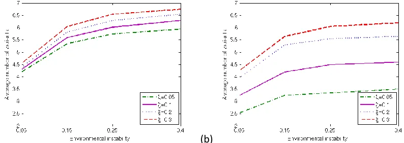
pattern for cultural diversity, with environmental variation promoting cultural variation. While the presence of a conformist bias reduces the average number of variants, individual learning increases it. We conclude that greater rates of environmental variability can be tackled by maintaining a higher number of cultural variants, which ensures that the population can respond adequately to a broad range of environmental conditions (cf. [29]).
[image:13.612.109.506.157.298.2](a) (b)
Figure 4. Average number of variants present in the population for different fractions of individual learning (dash-dotted line: ξ=0.05, solid line: ξ=0.1, dotted line: ξ=0.2, dashed line: ξ=0.3) and levels of conformity (left figure: b=0 and right figure: b=0.3).
Changes in environmental conditions may turn hitherto adaptive variants into variants with no functional utility (meaning ai(e(t,x))=0) (and vice-versa). Table 2 shows the average number of those
variants without utility in the population for the parameter set ε=0.4, b=0.3, for which an increase of the fraction of individual learning greatly improves the level of adaptation. Interestingly, while witnessing an increase in the adaptation level we simultaneously observe an increase in the number of non-beneficial variants. In other words, we obtain higher level of adaptations with increasing individual learning even though the number of non-beneficial variants is higher. This suggests that in frequently changing
environments, variants with no (or low) utility, if preserved, may play a role in the adaptation process by providing a reservoir of variation through which the population can adjust to new conditions (as
reported in [30]). If the environment is very unstable, variants conveying no benefit at this particular moment might become adaptive soon and can therefore accelerate the adaptation process, by conferring adaptive plasticity [30].
ξ=0.05 ξ=0.1 ξ=0.2 ξ=0.3
ε=0.4, b=0.3 0.37 0.56 0.83 1.25
Table 2. Average number of maladaptive variants in the population exposed to a changing environment.
We explored the characteristics of the variants that were most frequent in different spatial locations and concluded that the larger the width σi of the adaptation range of variant i the more likely it is that this
variant will be found in different locations x. Temporal instability in the environment favours the transmission of variants which are adapted to a broader range of environmental conditions, which can be seen as a generalist solution to the problem.
In summary, our analysis reveals that the more fluctuating the environment, the more
more that the environment fluctuates, the greater the number of cultural variants is expected to be present at the same time.
3.2.3 Effects of dispersal
Dispersal of the population is modelled as a diffusion process and therefore its direction is uncorrelated with the locations of the regions where the specific variants are beneficial. Consequently variants are carried into areas where they may or may not raise the adaptation level. We have seen in section 3.1 that in spatially variable but temporal constant environments dispersal did not lead to higher adaptation levels in the long run. If we add temporal variability then dispersal has a positive effect on the
population’s level of adaptation for a very small fraction of individual learning. Even though dispersal is undirected, it increases cultural diversity and can introduce new and well-adapted variants into certain spatial locations. Therefore it is able to facilitate the adaptation process in temporally changing
environments. However, with fractions of individual learning high enough to support the adaptation process, increasing dispersal rates result in reduced population levels of adaptation as variants are carried into areas where they might not be beneficial. Further, an increase of the dispersal rate lead to an increased strength of conformist bias in order to achieve the highest levels of adaptation in the population. In sum, the process of individual learning is far better suited than dispersal for ensuring an efficient adaptation process in temporally varying environments.
3.2.4 Effects of accuracy of individual learning
The accuracy of individual learning plays a crucial role in the evolution of conformity in temporally changing environments (cf. [9]). Naturally, more accurate individual learning will raise the adaptation level of the population. As the accuracy of individual learning increases, the adoption probability of a beneficial variant via individual learning increases, while the adoption probability of a less beneficial variant decreases. Now social learning acts on a set of variants that are better adapted to the experienced environmental conditions, which particularly benefits conformity. Due to the increased adoption probability of beneficial variants, individual learning is able to introduce those variants at higher frequencies. Following the line of argument developed in section 3.2, with more accurate individual learning the level of conformity can be higher before it acts to reduce the adaptation level by hindering or preventing well-adapted but low-frequency variants from spreading.
4
Applications of the approach
Frequency data can be obtained for many real world scenarios, although the temporal and/or spatial resolution may often be sparse. In the following, we explore how our model can be applied to frequency data and subsequently how it can be used to infer information about, for instance, the proportions of individual and social learning exhibited by the population, the level of conformity, and the adaptation levels of different cultural variants. To do this, we need to estimate the ranges of the model parameters determining the strength of those different processes, which result in frequency change pattern that are consistent with the observed variation. In general, this proves to be a difficult task especially for sparse data, where there are a large number of parameters, or where there is a complex likelihood surface for the model. Approximate Bayesian Computation (ABC) offers an elegant and efficient way around these problems. ABC has been developed to infer posterior distributions about unknown parameters if the likelihood function is either impossible or computationally prohibitive to obtain [22]. Those methods build on the computational efficiency of modern simulation techniques by replacing the calculation of the likelihood function with a comparison between the observed and calculated data. Toni et al. [34] have established the applicability of ABC methods to estimate the parameters of dynamical systems. In the following, we use a sequential Monte Carlo algorithm to estimate the parameters used in our model (see [3,34]). The idea is to find the range of parameter constellations that are most likely to have produced the observed frequency pattern under the assumed model and a given tolerance level. Based on those ranges we can draw conclusions about the adoption mechanisms used by the population.
[image:15.612.207.400.496.638.2]To demonstrate the applicability of this approach we aim to recover the parameters from noisy data produced by the model itself. We sample 10 data points of the frequencies of the cultural variants over time and add Gaussian noise N(0,σ2) (The standard deviation σ is assumed to be 20% of the data value). In this way we have full control over the real parameter values and can compare those to the estimated parameters. For sake of simplicity we assume a spatial homogeneous environment which experiences a shock at time t=50. Two variants are present during the first phase [0,50] and after the environmental change two further, better adapted, variants are introduced (cf. Figure 5 for the time course of the frequencies).
Figure 5. Time course of the frequencies of the four considered cultural traits (solid lines), and noisy data (squares), which are used as the input for the SMC method. Environmental change happens at time t=50.
We assumed that the parameter ri and cij depend explicitly on the level of adaptation of the specific
adaptation level ai of each variant. We assume no prior knowledge about the adoption situation and
therefore assume uniform priors for the adaptation levels ai, fraction of individual learning ξ and the
level of conformity b. Applying the sequential Monte Carlo (SMC) method yields to the posterior
[image:16.612.77.479.175.472.2]distributions of the relevant parameter for the time periods before and after the environmental change. Figure 6 shows the posterior distributions of the level of adaptation ai, i=1,…,4 of the four cultural
variants before (dark grey histograms) and after (light grey histograms) the environmental shock.
(a) (b)
(c) (d)
Figure 6. Posterior distributions of the level of adaptation ai of the four cultural variants (variant 1 (a), variant 2 (b), variant 3
(c) variant 4 (d)). Dark grey histograms describes the situation before the environmental change t= [0,50] and light grey histograms after the environmental change t=(50,100]. ‘True’ parametera1=0.3 (before), a1=0.1 (after); a2=0.45 (before),
a2=0.15 (after); a3=0.35; a4=0.45 are indicated by black vertical lines.
(a) (b)
Figure 7. Posterior distributions of (a) the fraction of the population relying on individual learning ξ and (b) the level of conformity b. Dark grey histograms describes the situation before the environmental change t= [0,50] and light grey histograms after the environmental change t=(50,100]. ‘True’ parameterξ=0.1; b=0 are indicated by black horizontal lines and the y-axis, respectively.
In summary, the application of ABC methods to observed data generates posterior distributions of the model parameters that indicate the parameter ranges which produce frequency pattern within a tolerance interval of the observed data. Importantly, the widths of those posterior distributions reflect the link between the model’s sensitivity for parameter change and the extent to which an accurate estimate of the parameter values can be inferred [34]. As already stated, the parameters determine the strength of different learning strategies in the adoption process and therefore a very broad posterior distribution would mean that not much information about the process can be extracted from the data (given the considered model). In contrast, a narrow distribution indicates that only a small range of parameter values is able to produce the observed frequency pattern. This correspondence between sensitivity and the ability to draw inferences is crucial. This is especially the case for complex models with a large number of parameters as ‘key’ model parameters will be quickly identified and possess narrow posterior distributions. Consequently the resulting posterior distributions allow us to evaluate the importance of the considered cultural processes in the adoption process.
We stress that we do not try to identify an unique adoption behaviour of the population, but rather seek to illustrate the potential of applying ABC methods to frequency data by quantifying credible parameter ranges and therefore by excluding large parts of the parameter space which are not
consistent with the observed data. This allows us, at the minimum, to infer (conditioned on the considered model) whether observed patterns of variations are consistent with high or low fraction of individual learning or whether the population shows weak or high conformist tendencies.
Naturally the value of this inference framework depends on the adequacy of the description of the temporal and spatial change patterns of the variant frequencies and the quality of the observed frequency data. Consequently a crucial element of our suggested analysis is to establish that the developed model does indeed capture the major processes responsible for the frequency change of the different cultural variants. Given the large number of competing models for the structure of the
underlying processes, it would be helpful to compare their performance in describing the observed data. To do so the SMC algorithm can be extended into a model selection framework (see [34]). This allows for the discrimination among a set of candidate models {m1,…,mn} in a formal Bayesian selection sense by calculating the probability pi with which model mi describes the data3 (holding p1+…+pn=1) and the
3
corresponding posteriori distributions of the model parameters. The subsequent calculation of the Bayes factors gives an indication of the support provided by the data in favour of one model over another [18]. We note that frequently there might not be a single best model; indeed, given the often sparse nature of the data and the complexity of interactions, this is to be expected. However, the described statistical inference framework can provide us with a greatly narrowed set of models and corresponding parameter ranges which are consistent with the observed data and therefore provides researchers with valuable information about which models and parameter ranges could not have produced the data. Moreover, while our analysis solely includes frequency information, other lines of evidence can be applied to this reduced set of models to narrow it down further.
5
Conclusion and discussions
We have developed a mathematical model to trace the changes in frequencies of different variants of a cultural trait in the face of individual and social learning of various forms, as well as dispersal, in a spatially and temporally variable environment. Our approach assumes that variants are differentially adapted to different environmental conditions. Changes in frequencies are caused by adoption decisions of the population, where the adoption probability of each variant is correlated to the benefit the variant conveys in a particular environment. We had two objectives. Firstly, we explored the relationship between individual and social learning and the population’s mean level of adaptation in changing environments, with a particular focus on conformity and on the role of cultural diversity in the process of adaptation. Secondly we investigated whether our model could be combined with statistical
techniques such as Approximate Bayesian Computation to infer information about learning strategies from usage or occurrence frequencies of different variants of a cultural trait.
Even though our model differs structurally from the gene-culture coevolutionary models (e.g. [5,11]), reassuringly our approach is validated by the confirmation of some basic and widely accepted results. For instance, we found, in accordance with the existing literature, a synergy effect between individual and social learning, such that in temporally changing environments, a mixture of individual and social learning leads to the highest level of adaptation. We can conclude that the outcomes of evolution maximizing individual and average fitness, respectively are similar.
Social learning can only act on variants that already exist at a given location which, in changing environmental conditions, might not be sufficient to ensure well-adapted populations. Individual
individual learning in our approach and we deduce that it might not be so important for the adaptation process which mechanism produces variation but only that variation is produced.
Generally speaking, individual learning provides the set of variants from which social learning can choose. The process of individual learning considered here is based on the inference between the experienced environmental conditions and the judgments about the utility of specific variants in those conditions. As this mapping is likely to be error-prone social learning can be seen as a mechanism that, amongst others, straightens out the errors. It is worth pointing out that even highly error-prone
individual learning (which can be seen as a random invention process) initiates adaptation. The strength of social transmission of a variant depends on judgements of its benefit (which is correlated to the variant’s adaptation level) and the variant’s frequency. Therefore social learning typically favours adaptive over non-adaptive variants, and in this way can greatly increase the population’s mean level of adaptation.
In frequently changing environments, the highest adaptation level of a population is obtained by a relatively high fraction of individual learning combined with high strength of conformity. This is in agreement with results obtained from analysing the properties of evolutionary stable strategies
([19,26,35]) and again the outcomes of evolution maximizing individual and average fitness, respectively are similar. More generally, we witness a tradeoff between the strength of conformist bias and the proportion of conformists in the population necessary to maintain high levels of adaptation. This relationship is caused by the opposing effects of conformity and individual learning on low-frequent variants. While conformity hinders or even prevents the spread of low-frequent variants individual learning has the capacity to introduce new variants usually at low frequency, counteracting the diversity-reducing tendency of conformity. A weak conformity bias requires only a small fraction of individual learners to counteract its negative effects, while a strong conformity bias requires a larger fraction if adaptive variants are not to be suppressed. These observations imply a limit on the amount of conformity that can be maintained within a population, as represented by an upper bound to the product of the proportion of conformists and the strength of the conformity bias. These theoretical findings are consistent with recent experimental evidence characterizing humans as ‘conformists’ or ‘mavericks’ (i.e. individual learner) [9] and revealing considerable variation amongst individuals in their tendency to conform and use social information [25].
Our study points to the crucial role cultural diversity, and consequently the mechanisms creating diversity, play in an effective process of adaptation to changed environmental conditions. Populations that show high levels of adaptation in frequently changing environments are characterized by high levels of cultural diversity (as, for example, expressed by a high average number of present variants covering a broad range of possible conditions). This finding suggest that maintaining a diverse portfolio of solutions that offer different benefits in different environmental settings to a problem, even to the extent of keeping temporally maladaptive variants in the portfolio, provides an efficient way to adapt to frequently changing environments (see also [30]). We also found that variants that are adapted to a broader range of environmental conditions are found more frequently in the portfolios of different spatial locations. Therefore one should expect that generalist solutions to a problem are favoured over specialist solutions in frequently changing conditions.
climatic variation. We add to this argument that not only culture, but diverse culture encompassing a set of variants covering a broad enough range of environmental conditions, is needed in order to ensure an efficient adaptation process.
Finally, we note that often researchers (e.g. archaeologists, biological anthropologists,
psychologists) are confronted with situations where time series data is available detailing the usage or occurrence of different cultural variants, and where they would benefit from being able to infer
something about the underlying social processes that produced those frequencies. As our approach links frequency change patterns of cultural variants with the adoption decisions of the population it
potentially informs such inference. We envision that our model, in combination with the described ABC methods, could shed some light into this problem. The model parameters determine the strength of the different adoption processes and therefore the resulting posterior distributions of those parameters allow us to draw conclusions about the adoption mechanisms manifest in the population. However, especially with sparse data we do not claim the existence of a unique relationship between observed frequency patterns and underlying processes; to the contrary, we expect that different processes will be consistent with the observed frequency patterns. Nonetheless, we anticipate that our approach will be valuable in helping to narrow down the range of possible processes that could have produced those patterns, and thus will still be instructive in the face of uncertainty.
Acknowledgements
This research supported by an Omidyar Fellowship from the Santa Fe Institute to AK and an ERC Advanced grant to KNL. We thank two anonymous reviewers for their comments which helped improving this paper.
References
[1] K. Aoki, J.Y. Wakano, M.W. Feldman, The emergence of social learning in a temporally changing environment: a theoretical model, Curr. Anthropol. 46 (2005) 334-340.
[2] K. Aoki, W. Nakahashi, Evolution of learning in subdivided populations that occupy environmental heterogeneous sites, Theor. Popl. Biol. 74 (2008) 356-368.
[3] M.A. Beaumont, Approximate Bayesian computation in evolution and ecology, Annu. Rev. Ecol. Evol. Syst. 41 (2010) 379-406.
[4] R. Boyd, P.J. Richerson, Culture and the evolutionary process. Chicago: The University of Chicago Press, 1985.
[5] R. Boyd, P.J. Richerson, An evolutionary model of social learning: the effect of spatial and temporal variation, In: Zentall T., Galef, Jr., B.G. (eds) Social learning. Erlbaum, Hillsdale, NJ, 1988.
[7] T. Day, P.D. Taylor Evolutionary stable versus fitness maximizing life histories under frequency-dependent selection, Proc. R. Soc. Lond. B. 263 (1996) 333-338.
[8] L. Cronk, That complex whole: culture and the evolution of human behavior, Westview Press, 1999.
[9] C. Efferson, R. Lalive, P.J. Richerson, R. McElreath, M. Lubell Conformists and mavericks: the empirics of frequency-dependent cultural transmission, Evol. Hum. Behav. 29 (2008) 56-64.
[10] K. Eriksson, M. Enquist and S. Ghirlanda, Critical points in current theory of conformist social learning, Journal of Evolutionary Psychology. 5:1-4 (2007) 67-87.
[11] M.W. Feldman, K. Aoki, J. Kumm, Individual versus social learning: Evolutionary analysis in a fluctuating environment, Anthropol. Sci. 104 (1996) 209:232.
[12] J.B. Haldane The causes of evolution. Harper and Brothers, London, 1932.
[13] J. Henrich, Cultural transmission and the diffusion of innovations: Adoption dynamic indicate that biased cultural transmission is the predominant force in behavioural change, American Anthropologist. 103:4 (2001) 992-1013.
[14] J. Henrich, R. Boyd, The evolution of conformist transmission and the emergence of between-group differences, Evol. Hum. Behav. 19 (1998) 215-241.
[15] Heyes C.M., Social learning in animals: categories and mechanisms, Biol. Rev. 69 (1994) 207-231.
[16] J.S. Huxley The present standing of the theory of natural selection. In: G.R. deBeer (ed.) Evolution. Clarendon Press, Oxford, 1938.
[17] A. Kandler, K.N. Laland, An investigation of the relationship between innovation and cultural diversity, Theor. Popul. Biol. 76 (2009) 59-67.
[18] R.E. Kass and A.E. Raftery, Bayes factores, J. Am. Statist. Assoc. 90:410 (1995) 773-795.
[19] J. Kendal, L.-A. Giraldeau, K.N. Laland, The evolution of social learning rules: Payoff-biased and frequency-dependent biased transmission, J. Theor. Biol. 260 (2009) 210-219.
[20] K.N. Laland, Social learning strategies, Learn. Behav. 32:1 (2004) 4-14.
[22] P. Marjoram, P. Molitor, J. Plagnol, S. Tavare, Markov chain Monte Carlo without likelihoods, Proc. Natl. Acad. Sci. 100 (2003) 15324-15328.
[23] J. Maynard Smith, Optimization theory in evolution. Annual review of ecology and systematics. 9 (1978) 31-56.
[24] R. McElreath, B. Fasolo, A. Wallin, The evolutionary rationality of social learning, In: R. Hertwig, U. Hoffrage and the ABC Research Group (Eds.), Simple Heuristics in a Social World, Oxford University Press, 2011.
[25] T.J.H. Morgan, L. Rendell, M. Ehn, W.J.E Hoppitt, K.N. Laland, The evolutionary basis of human social learning, Proc. R. Soc. B 279:1729 (2012) 653-662.
[26] W. Nakahashi, The evolution of conformist transmission in social learning when the environment changes periodically, Theor. Popul. Biol. 72 (2007) 52-66.
[27] W. Nakahashi, J.Y. Wakano, J. Henrich, Adaptive Social Learning Strategies in Temporally and Spatially Varying Environments, Human Nature 23 (2012) 386-418.
[28] L. Rendell, L. Fogarty, K.N. Laland, Rogers’ paradox recast and resolved: Population structure and the evolution of social learning strategies, Evolution 64(2) (2010) 534-548.
[29] L. Rendell, R. Boyd, D. Cowden, M. Enquist, K. Eriksson, M.W. Feldman, L. Fogarty, S. Ghirlanda, T. Lillicrap, K.N. Laland, Why copy others? Insights from the Social learning Startegies Tournament, Science 328:5975 (2010) 208-213.
[30] L. Rendell, R. Boyd, M. Enquist, M.W. Feldman, L. Fogarty, K.N. Laland, How copying affects the amount of eveness and persistence of cultural knowledge: insights from the social learning strategies tournament, Phil. Trans. R. Soc. B 366:1567 (2011) 1118-1128.
[31] A.R. Rogers, Does biology constrain culture? Am. Anthropol. 90 (1988) 819-831.
[32] P.J. Richerson, R. Boyd, Built for speed: Pleistocene climate variations and the origins of human culture. Perspect. Ethol. 13 (2000) 1-45.
[33] P.J. Richerson, R. Boyd, Not by genes alone, The University of Chicago Press, Chicago and London, 2005.
[35] J.Y. Wakano, K. Aoki, Do social learning and conformist bias coevolve? Henrich and Boyd revisited, Theor. Popul. Biol. 72 (2007) 504-512.
[36] J.Y. Wakano, K. Aoki, M.W. Feldman, Evolution of social learning: a mathematical analysis, Theor. Popul. Biol. 66:3 (2004) 249-258.
[37] O. C. Zienkiewicz and R. L. Taylor The Finite Element Method: Its Basis And Fundamentals, fourth ed., MacGraw-Hill London, 1991.