Conservative reasoning about epistemic uncertainty for the probability of failure on demand of a 1-out-of-2 software-based system in which one channel is "possibly perfect"

City, University of London Institutional Repository

Citation

:

Littlewood, B. and Povyakalo, A. A. (2012). Conservative reasoning about epistemic uncertainty for the probability of failure on demand of a 1-out-of-2 software-based system in which one channel is "possibly perfect" (CSR Technical Report 20 March 2012). London: Centre for Software Reliability, City University London.

This is the unspecified version of the paper.

This version of the publication may differ from the final published

version.

Permanent repository link:

http://openaccess.city.ac.uk/1611/

Link to published version

:

CSR Technical Report 20 March 2012

Copyright and reuse:

City Research Online aims to make research

outputs of City, University of London available to a wider audience.

Copyright and Moral Rights remain with the author(s) and/or copyright

holders. URLs from City Research Online may be freely distributed and

linked to.

probability of failure on demand of a 1-out-of-2 software-based

system in which one channel is “possibly perfect”

Bev Littlewood, Andrey Povyakalo

Centre for Software Reliability, City University, London

Abstract

In earlier work, (Littlewood and Rushby 2011) (henceforth LR), an analysis was presented of a 1-out-of-2 system in which one channel was “possibly perfect”. It was shown that, at the aleatory level, the system pfd could be bounded above by the product of the pfd of channel A and the pnp (probability of non-perfection) of channel B. This was presented as a way of avoiding the well-known difficulty that for two certainly-fallible channels, system pfd cannot be expressed simply as a function of the channel pfds, and in particular not as a product of these. One price paid in this new approach is that the result is conservative – perhaps greatly so. Furthermore, a complete analysis requires that account be taken of

epistemic uncertainty – here concerning the numeric values of the two parameters pfdA and pnpB. This introduces some difficulties, particularly

concerning the estimation of dependence between an assessor’s beliefs about the parameters. The work reported here avoids these difficulties by obtaining results that require only an assessor’s marginal beliefs about the individual channels, i.e. they do not require knowledge of the dependence between these beliefs.

1

Introduction

Intellectual diversity has been used from time immemorial to improve the dependability of human activities. Most people believe that, for many activities, “two heads are better than one”: e.g. it is often better to have another person check your work than to do it yourself. The use of diversity to build reliable systems long pre-dates the use of computers. For example, the use of diverse multi-channel safety protection systems based on physically different variables (temperatures, pressures, flow-rates…) has for a long time been an attractive design approach.

The intuition here is very simple. We must expect that humans will make mistakes when designing and building systems, and that these mistakes will eventually result in failures of the systems during operation. But if we force two or more systems to be built differently, their resulting failures may also be different. So if, in a 1-out-of-2 protection system, channel A fails on a particular demand, there may be a good chance that channel B will not fail.

safety-critical flight control systems of Airbus fleets (Rouquet and Traverse 1986) have experienced massive operational exposure (Boeing 2010) with apparently no critical failure. We might conclude that these systems are very reliable (although we are not aware that any figures have been published that would tell us how reliable).

However, there remain serious difficulties in assessing the reliability of such systems before operational use. The stringent dependability requirements for safety-critical systems – e.g. 10-9

probability of failure per hour for critical avionics systems in civil aircraft (FAA 1988; RTCA 1992) – usually mean that black-box operational testing would require infeasible times on test (Butler and Finelli 1993; Littlewood and Strigini 1993). Furthermore, it is well-known that it is not possible to claim, with certainty, independence between the failures of multiple software-based channels of a system: see (Knight and Leveson 1986; Eckhardt, Caglayan et al. 1991) for experimental evidence, and (Eckhardt and Lee 1985; Littlewood and Miller 1989) for theoretical reasons for this assertion. In fact in general for a 1-out-of-2 demand-based system it must be assumed that

pfd_sys>pfd_A×pfd_B (1)

because there will usually be positive association between the failures of channel A and those of channel B.1 _{So, for example, if the two channels of a 1-out-of-2 system each} have probability of failure on demand (pfd) 10-3

, it would be wrong to claim prima facie a pfd of 10-6

for the system. In fact, statistical independence is probably a rather rare phenomenon in the world: see (Kruskal 1988) for an amusing but serious discussion of inappropriate assumptions of independence.

If independence cannot be assumed between channel failures, the problem of assessing the reliability of the system becomes difficult: we need to know how dependent the failures of the channels are. All this was formalized some years ago with the introduction of the “difficulty function” (Eckhardt and Lee 1985; Littlewood and Miller 1989). This can be thought of as a function θ(x) over the demand space, representing the probability that a randomly selected program fails on demand x: i.e. demands with a large value can be thought of as more failure-prone, or “difficult”. Typically, the difficulty functions for channels A and B will be different because they have been “built differently”. It is shown in (Littlewood and Miller 1989) that the probability of system failure on a randomly chosen demand is

pfdsys=pfdA×pfdB+Cov(θA,θB) ₍₂₎

So an assessor’s beliefs about the channel reliabilities are not sufficient for them to reason about the system reliability: they also need to know the covariance of the difficulty functions, which is unlikely to be known.

1 _{Whilst negative association is theoretically possible (Littlewood, B. and D. R. Miller (1989). "Conceptual Modelling}

of Coincident Failures in Multi-Version Software." IEEE Trans on Software Engineering 15(12): 1596-1614.) – thus reversing the inequality in (1) – we are not aware of any means of claiming this with high confidence in a particular instance.

2 _{This kind of reasoning is more common at the aleatory level. We have seen arguments in which pessimistic claims}

It is this problem of assessing how dependent the channel failures are that lies at the heart of multi-channel system dependability assessment. The individual channel pfds can be estimated from operationally representative statistical testing, so long as the levels required are reasonably modest. If we could assume failure independence, strong claims could be made about the system pfd from modest channel pfds, simply by multiplying them. But in the absence of independence, it is necessary know how dependent the channel failures are – represented by the covariance term above. Estimating this, e.g. from testing, seems as hard as estimating the system pfd directly, and this is known to be infeasible in those cases where very high system reliability is required.

This presents us with an impasse. Whilst there is plentiful evidence that the multi-version approach is effective, at least in some average sense, in achieving high reliability, we cannot assess the reliability of a particular such system. Such assessment does seem essential, of course, when these systems are critical and their failure may involve the loss of life.

In recent work, a way around this difficulty has been proposed for certain special architectures (Littlewood and Rushby 2011). The idea here is that in some 1-out-of-2 systems, one channel (say A) may be highly functional and complex, and so (effectively certainly) failure-prone, but the other channel (B) may be very simple and thus possibly perfect. By “perfect” we mean that this channel cannot fail in its entire life, no matter how much exposure it receives, i.e. its pfd is zero. By “possibly perfect” we mean that such perfection will not be known with certainty. Claims about A will be expressed as a probability of failure on a randomly selected demand (pfdA); claims about B will be expressed as a probability that it is not perfect (pnpB).

The key idea in LR is that, at the aleatory level, it can be shown that there is conditional independence between the events “A fails on a randomly selected demand” and “B is not perfect,” given that the probabilities of these events, respectively pfdA and pnpB, are known. It is then shown that a conservative bound for the system’s (conditional) probability of failure on demand is simply the product of the probabilities of these two events, i.e.

pfd_sys≤pfd_A×pnp_B (3)

where the conservatism arises by assuming that, if B is imperfect, it always fails when A does. See (Littlewood and Rushby 2011) for proof. An assessor can then use the right hand side of (3) for the probability of failure on demand of the system, and be confident that this is conservative.

In other words, when pfdA and pnpB are known, they are jointly sufficient for computing an upper bound on the value of pfdsys. The important point here is that there is no equivalent simplification in the case where both channels must be assumed to be fallible – it is not sufficient to know pfdA and pfdB. In addition, knowledge of the nature of the dependence between the channel failures is also needed: see (2).

to the one we would use if we could assume channel failures to be independent (the product of two small channel pfds).

So far the discussion here has concerned only aleatory uncertainty, or “uncertainty in the world”. In reality, of course, none of the values of the parameters in this discussion will be known with certainty. This is where epistemic uncertainty – or “uncertainty about the world” – comes in, as a result of the imperfect knowledge of the assessor. In LR the assessor beliefs are represented formally by a distribution:

F(pA,pB)=P(pfdA<pA,pnpB <pB) (4)

which is best thought of as a Bayesian posterior distribution that incorporates all the evidence that the assessor has about the unknown parameters.

The assessor’s probability of system failure on a randomly selected demand is then bounded by the posterior mean of the product, from (3):

pA×pBdF(pA,pB)

0≤p_A≤1 0≤p_B≤1

∫

(5)

The value of the LR approach, compared with one that treats each channel as certainly fallible, is two-fold. Firstly – at the aleatory level – we can multiply two small numbers together to obtain a (conditional, conservative) small probability of failure on demand for the system. Secondly, at the epistemic level things are simpler because an assessor “only” needs to express his beliefs as a bivariate distribution, (4). In contrast, in the earlier case, he would need to express his beliefs as a three dimensional distribution for the two channel pfds together with the difficulty covariance, (2). As we have remarked, information about the covariance is unlikely to be available. Furthermore, the assessor would be unlikely to be able to express his beliefs about the dependencies between the three parameters.

Nevertheless, in spite of the simplification that LR brings, the assessor faces a difficult challenge in expressing his beliefs in a distribution, (4). It is this problem that we address in the rest of the paper.

If F factorised, i.e. the assessor’s beliefs about the two parameters were independent, then (5) would simplify into the product of the means of the posterior marginal distributions of the parameters. Unfortunately, assessors’ beliefs are unlikely to be independent in this way, and this epistemic dependence poses a serious problem.

In (Littlewood and Rushby 2011) a way of conservatively simplifying (5) is proposed. Here, the notion of “possibly independent” is introduced: the assessor has a probability (1-C) that there do not exist any factors inducing dependence (and consequently a probability C that there is dependence). The analysis proceeds conservatively by assuming that, in the event that there is dependence, the system fails with certainty on a randomly selected demand. It is shown that system pfd can be bounded as follows:

P(system fails on randomly selected demand)

≤C+(1−C)× p_A×p_BdF(p_A,p_B) 0≤p_A<1

0≤p_B<1

€

=C+(1−C)×P_A*

×P_B* ₍₇₎

where PA* and PB* are the means of the posterior distributions representing the assessor’s beliefs about the two parameters, each conditional on the parameter not being equal to one (i.e. A not certain to fail, B not certain to be imperfect).

If C is small (as is likely in the contexts in which such reasoning takes place in real life), (1-C) is approximately 1, and we can substitute the unconditional posterior marginal means, PA and PB, into (7) to yield the conservative approximation:

C+PA×PB (8)

See (Littlewood and Rushby 2011) for a detailed discussion about this.

As we have remarked, this approach is considerably simpler at the aleatory level than one that treats both channels as fallible, because of the great difficulties associated with estimating the dependence between channel failure processes. However, it has to be said that the estimation problem at the epistemic level here is hard, even though it is also much simpler than the corresponding one for the case of two fallible channels.

The parameter for which it is easiest for an assessor to obtain an estimate is PA, the probability of failure on demand of channel A. There is a large literature, for example, on operational testing, from which a direct estimate, and confidence bounds, can be obtained: see (May, Hughes et al. 1995), for an example of estimating the pfd of a channel of a real nuclear protection system, and (Littlewood and Wright 1997) for a Bayesian treatment. This kind of evidence can often be augmented from less direct sources, such as the quality of the processes used to build the system, or of the experience of the team involved, etc.

The parameter PB, the probability that channel B is not perfect, poses some difficulties: see (Littlewood and Rushby 2011) for an extensive discussion about this issue. (Littlewood and Wright 2007) show how testing and verification evidence can be used, via a Bayesian Belief Net (BBN), to obtain confidence in perfection of a channel. We shall report elsewhere on some of our recent work on this problem.

Finally, the parameter C seems to present the hardest problem. Judging dependence between random variables seems to be a harder task for people than judging marginal mean values, or marginal percentiles. In addition, there is usually a paucity of evidence to support claims about dependence (or independence). The problem seems particularly difficult in the case of epistemic dependence, as here.

The aim of the current paper is to devise ways around this latter difficulty. In the next sections we present different approaches that avoid the need to estimate dependence. These new results rely solely upon assessors’ marginal beliefs about the individual channel parameters – pfdA, pnpB – and do not require epistemic dependence between them to be estimated. There is a price paid, not surprisingly, for this simplification: further conservatism is introduced into the claims that can be made about the system pfd. Nevertheless we believe that these new bounds will be of practical utility.

2

Conservative bounds on mean system

pfd

We begin with the result (3). Instead of dealing with the complete bivariate distribution, (4), representing the assessor’s posterior beliefs about the parameters pfdA and pnpB, we shall assume only that the assessor can tell us something about his separate marginal distributions for these parameters, which we shall call F(pA) and F(pB) in an obvious notation. Clearly this places upon the assessor a much less onerous requirement in describing his epistemic uncertainty, inasmuch as he does not need to say anything about the dependence in his beliefs about the parameters.

Initially, we assume that the assessor is able to give us only a single percentile for each distribution:

€

P(pfdA< pA)=1−αA P(pnpB < pB)=1−αB

(9)

So pA is his 100(1-αA)% upper confidence bound for the parameter pfdA; equivalently, αA can be thought of as his doubt that pfdA is smaller than pA, etc.

We have the following:

Theorem 1

If

€

P(pfd_A< p_A)=1−αA and P(pnpB< pB)=1−αB

represent the assessor’s marginal posterior beliefs about the parameters, and without loss of generality

€

αA≤αB, then

€

E(pfd_sys)≤p_A×p_B×(1−αB)+pA×αB+(1−pA)×αA (10)

Proof

Denote the unknown joint probability,

€

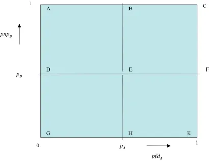
P(pfdA >αA,pnpB>αB), i.e. of lying in BCFE in

Figure 1, by z. Now pfdsys≤E(pfdA×pnpB)

= p_A×p_B×(1−αA−αB+z)+pA×(αB−z)+pB×(αA−z)+z (11)

= pA×pB×(1−αA−αB)+αA×pB+αB×pA+z×(1−pA−pB+pA×pB)

€

≤ pA×pB×(1−αA−αB)+αA×pB+αB×pA+min(αA,αB)×(1−pA−pB+pA×pB)

€

= pApB(1−αB)+pAαB+(1−pA)αA because

€

€

[image:8.612.99.509.126.447.2]

1−pA−pB+pA×pB≥0

Figure 1. The random variable (pfdA,pnpB) is defined on the unit square. Note that

this figure has been exaggerated for clarity: in reality E would be very close to the origin.

The result (11) can be seen as follows. Consider the four rectangles in Figure 1: DEHG, ABED, EFHK, BCFE. The product

€

pfdA×pnpB is a random variable which is everywhere smaller than

€

pA×pB within DEHG. The probability associated with DEHG is

€

(1−αA−αB+z). Thus the contribution to

€

pfd_sys =E(pfd_A×pnp_B) associated with DEHG is bounded above by the product

€

pA×pB×(1−αA−αB+z). Hence the first term

in (10). Similarly, within the rectangle ABED, the product

€

pfdA×pnpB is a random

variable which is everywhere smaller than pA (which value it takes at the point B); and the probability associated with this rectangle is

€

(αB−z); so the contribution to the mean

of this rectangle is bounded by the product of these. Hence the second term in (11). Similar reasoning about EFHK, BCFE give the third and fourth terms of (11), respectively.

Example 1

If the assessor can provide a single percentile (i.e. a bound with associated confidence level) for each marginal posterior distribution (i.e. for pfdA and for pnpB) then the theorem provides a means of computing a conservative posterior mean of pfdsys.

So, if the assessor is 95% confident that pfdA is smaller than 10-5

, and 95% confident that pnpB is smaller than 10-2

we have, from (10):

€

E(pfd_sys)≤10−5 ×10−2

×(1−0.05)+10−5

×0.05+(1−0.05)×0.05≈0.05 (12)

which of course is very conservative.

If the assessor is 99% confident that pfdA is smaller than 10-3

, and 99.9% confident that pnpB is smaller than 10-1

, the bound on his posterior mean for the system pfd is about

€

1.1×10−3

.

In fact, since “doubts” will usually be considerably greater than “claims”, this way of bounding the assessor’s posterior pfd for the system will give a result that is approximately the same as the smallest of the two doubts.

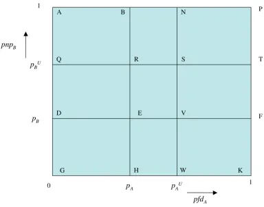
So these results are very conservative. One reason for this is that it is assumed that there is probability mass over the whole unit square: that is, the assessor cannot rule out the possibility of the parameters taking any value. This probability mass is assigned most pessimistically in each of the rectangles making up the unit square, e.g for the random variable (pfdA, pnpB) lying in the upper right rectangle, all probability is assigned to the point (1,1), i.e. it is assumed with this probability that channel A fails, and channel B is imperfect, so that the system fails with certainty. This is similar to the LR reasoning. Such beliefs may be too pessimistic for real assessors. An assessor may say: “I have confidence (1-αA) that channel A’s pfd is smaller than pA, but I am certain that it is smaller than pA

U

, where pA<<pA U

”, with similar certainty that pnpB is smaller than pB U

. This is illustrated in Figure 2, where now there is non-zero probability mass only in the rectangle QSWG: outside this rectangle the distribution (4),

€

F(pA,pB), takes the value 1

everywhere.

We can now obtain a tighter conservative bound as follows:

Theorem 2

If

€

P(pfdA< pA)=1−αA and P(pnpB< pB)=1−αB and

€

P(pfd_A< p_AU)=1 and P(pnp_B <p_BU)=1

represent the assessor’s marginal posterior beliefs about the parameters, and without loss of generality

€

αA≤αB,

€

E(pfdsys)≤pA×pB×(1−αB)+pA×pB U

×αB+pB U

×(pA U

−pA)×αA (13)

Figure 2. As Figure 1, except that now, in addition, the assessor is certain that pfdA does not exceed pAU and pnpB does not exceed pBU. So there is zero

probability mass outside QSWG.

Proof

This is similar to the proof of the previous theorem, in terms of the four rectangles making up QSWG. Once again, denote by z the unknown probability mass associated with RSVE.

In DEHG, the random variable pfdApnpB is bounded above by pApB and the probability mass here is (1-αA-αB+z). So the contribution of DEHG to the posterior mean of the system pfd is bounded above by pApB(1-αA-αB+z).

By similar reasoning, the contribution from QRED is bounded by pApB U

(αB-z); that from EVWH by pA

U

pB(αA-z); that from RSVE by pA U

pB U

z.

Adding all these contributions together, and using the fact that

€

0≤z≤min(αA,αB)=αA,

[image:10.612.97.481.134.435.2]

Notice that, as expected, (13) reduces to (10) when pA =pB =1.

Example 2

As Example 1 with, additionally, pA U

=10-3 , pB

U =10-1

.

€

E(pfd_sys)≤10−7

×0.95+10−4

×0.05+0.05×(10−3 −10−5

)×10−1

≈0+0.5×10−5

+0.5×10−5

€

=1×10−5

(14) Clearly this is better than the bound in Example 1. And it is an order of magnitude improvement on the very crude bound that simply multiplies the two marginal upper bounds, i.e. 10-4

.

We now obtain some conservative bounds for the system pfd for situations in which the assessor knows the first two moments of his marginal distributions for the parameters, rather than percentiles as above:

Theorem 3

E(pfdsys)≤E(pfdA×pnpB)

< E(pfdA)

2

+Var(pfdA)

(

)

. E(pnpB)

2

+Var(pnpB)

(

)

!

" #$ ₍₁₅₎

<

(

E(pfdA)+SD(pfdA)

)

.

(

E(pnpB)+SD(pnpB)

)

₍₁₆₎

Proof

By the Cauchy-Schwarz inequality

E(pfdA.pnpB)

(

)

2 <E(pfdA

2

).E(pnpB 2

)

= E(pfd_A)2

+Var(pfd_A)

(

)

. E(pnp_B)2

+Var(pnp_B)

(

)

which gives (15). And

E(pnp_B)2

+Var(pnp_B)<

₍

E(pnp_B)+SD(pnp_B)

₎

2

with a similar expression involving pnpB, so (16) follows.

Example 3

The result requires knowledge of the first two moments of the marginal distributions of the two model parameters. In particular, the closeness of the bound to the “ideal” independence result (i.e. product of the marginal means of the parameters) depends on the relative sizes of the marginal standard deviations and marginal means. So, if

we have

E(pfdsys)<25. E(pfdA). E(pnpB)

Another way in which (16) might be used is as follows. One way that we have heard assessors reason in the presence of difficult-to-assess dependence is to make a trade-off between “lack of independence” and “pessimism of channel claims”. The reasoning is something like this: “I realize I cannot simply multiply my marginal beliefs about the pfd of channel A and the pnp of channel B to obtain a bound for the system pfd, so I will instead multiply together pessimistic values for these two channel beliefs. The pessimism here will counteract the optimism of the independence assumption implicit in the simple multiplication of the numbers2_{.” The result (16) provides a formalism for this kind of} reasoning. It shows how much pessimism is needed to justify such reasoning: a system claim made in this way will be a conservative one if each channel claim is conservative by an amount equal to the standard deviation of the marginal distribution.

Finally, we present conservative bounds for the situation where an assessor’s beliefs about the two marginal distributions involve both means and percentiles as follows:

Theorem 4

If

P(pfdA >pA)=αA and P(pnpB>pB)=αB

and

E(pfdA)≤pA and E(pfdB)≤pB

then

E(pfdsys)≤E(pfdA×pnpB)

(17)

≤ pA×pB

αA×αB

(18)

Proof

We require the following

Lemma:

2 _{This kind of reasoning is more common at the aleatory level. We have seen arguments in which pessimistic claims}

have been made for each channel pfd and then these have been multiplied together to obtain a figure for the system pfd. The trade-off here is between channelfailure dependence and channel pfd pessimism. See Bishop, P., R. Bloomfield, et al. (2011). "Towards a formalism for conservative claims about the dependability of software-based systems." IEEE Trans Software Engineering 35(5): 708-717.

If

0≤X≤1, and P(X>p)=α, and E(X)≤p, then

E(X2

)≤E(X) 2

α ≤

p2

α

Proof: see appendix

From the lemma we have:

E(pfdA

2

)≤E(pfdA)

2

αA

≤ pA

2

αA and

E(pnpB

2

)≤ E(pnpB)

2

αB

≤ pB

2

αB

And by the Cauchy-Schwarz inequality:

E(pfdA×pnpB)≤ E(pfdA

2

)×E(pnpB

2

)

from which the result follows.

Example 4

If the assessor has a single percentile for each marginal distribution, as in Example 1:

pA=10-5

, αA=0.05, and pB=10-2

, αB=0.05

and the assessor is certain that E(pfdA)≤pA and E(pnpB)≤pB, then

E(pfdsys)≤ 10−5

×10−2

0.05×0.05 =2×10 −6

Obviously this is a tighter bound than in Example 1, using Theorem 1. In general, bounds (17) and (18) will be better than (10) and (13) whenever αA >>pA and αB >>pB, which will generally be the case (claims will usually be much smaller numerically than doubts). In fact it is even tighter than the bound in Example 2. At first glance this is surprising, since the latter requires the assessor to know with certainty upper bounds on the parameters, in addition to a percentile for each. The result here, however, similarly depends upon the assessor being certain that the marginal means are smaller than pA, pB respectively. This is so even though the weaker bound of Theorem 4, (18), which is used in the example, does not depend on the numerical values of these marginal means.

In summary, the assessor does not need to know both the marginal means and the percentiles to use the theorem. Useful bounds on system pfd can be obtained by knowing either

(a) E(pfdA), E(pnpB), αA, αB for result (17)

(b) pA, pB, αA, αB for result (18)

but in each case he must be certain that, in addition, the marginal means are smaller than the corresponding percentiles(even if the exact values of some of these are not known to him).

Of the two options, (a) gives the tighter bound and thus can be regarded as preferable in those cases where the assessor knows each of E(pfdA), E(pnpB), αA, αB, pA, pB. In both

cases, the bounds will be tighter for larger values of αA, αB. But of course larger values

of αA, αB are associated with smaller values of pA, pB, and if these are too small the bounds on the marginal means in Theorem 4 will be violated.

The tightest bound would occur if the assessor’s percentiles (pA, pB) coincided exactly with his marginal means E(pfdA), E(pnpB) - in which case (a) and (b) give the same

bound. Is it feasible that an assessor would be able to make them coincide in this way? In some cases an assessor may be prepared to specify a complete marginal distribution for each parameter (e.g. by accepting a parametric family, such as a 2-parameter Beta distribution, that is “fixed” by the determination of two percentiles – see Section 3). In that case the assessor will know E(pfd_A), E(pnp_B), he can choose pA, pBto coincide with these values, and then compute the corresponding αA, αB which will give the tightest bound.

3

Confidence bounds for system

pfd

A different approach from the above obtains conservative confidence bounds for the system pfd, again without requiring estimation of the dependence of the assessor’s beliefs about the unknown parameters pfdA and pnpB.

As before, we assume that the expert can provide a marginal percentile for each parameter, as in (9). We again use the LR result concerning aleatory uncertainty.

Given these beliefs of the assessor concerning the individual channels of the 1-out-of-2 system, we are interested in obtaining a confidence bound for the systempfd. That is, we want to evaluate the probability

€

P(pfd_sys <p_sys) (19)

for some value of psys.

Theorem 5

Given the confidence bounds in (9), i.e.

€

P(pfd_A <p_A)=1−αA

P(pnp_B< p_B)=1−αB

we have

€

Proof:

From (2)

€

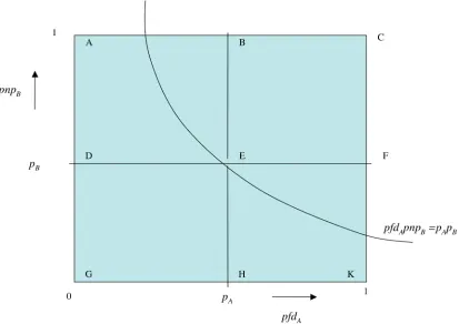
P(pfd_sys <p_A×p_B)>P(pfd_A×pnp_B <p_A×p_B) (21)

Now

€

P(pfdA×pnpB >pA×pB)

<P(pfdA> pA)+P(pnpB >pB)−P(pfdA >pA,pnpB> pB)

(22)

[image:15.612.99.512.284.576.2]

This is because the left hand side is the probability mass associated with the area above the hyperbola in Figure 3; this is smaller than the probability mass associated with the L-shaped region comprising rectangles ABED, BCFE, EFKH; which in turn is equal to probability masses of BCKH plus ACFD minus BCFE; these three probability masses correspond to the three terms on the RHS of (22), in the same order.

Figure 3. Essentially as Figure 1. Here the probability mass associated with the area below the hyperbola, pfdApnpB= pApB, corresponds to the probability on the

right hand side of equation (17).

€

P(pfd_A×pnp_B >p_A×p_B)<P(pfd_A >p_A)+P(pnp_B >p_B) (23)

So finally

€

P(pfd_sys <p_A×p_B)>P(pfd_A×pnp_B <p_A×p_B)

=1−P(pfd_A×pnp_B >p_A×p_B)

€

>1−P(pfdA> pA)−P(pnpB >pB)=1−(αA+αB) which completes the proof.

Informally, the theorem states that the system claim is the product of the channel claims

(p_A×p_B), and the doubt in this system claim is simply the sum of the channel claim doubts (αA+αB).

Example 5

For example, if he is 95% confident (5% doubt) that pfdA is smaller than 10

-5_{, and 95%} confident (5% doubt) that pnpB is smaller than 10-2

, then he is at least 90% confident (5%+5%=10% doubt) that pfdsys is smaller than 10-7

.

Example 6

If the assessor can provide two (or more) percentiles for each distribution, then multiple conservative percentiles can be generated for the distribution of pfdsys. So if, in additon to the two percentiles above, the assessor is 99% confident that pfdA is smaller than 10-3

, and 99.9% confident that pnpB is smaller than 10-1

, the following conservative percentiles apply to his beliefs about the system pfd:

1. Pfdsysis smaller than 10 -4

with 98.9% confidence (doubt = 1.1%) 2. Pfdsysis smaller than 10

-5

with 94% confidence (doubt = 6%) 3. Pfdsysis smaller than 10

-6 _{with 94.9% confidence (doubt = 5.1%)}

4. Pfdsysis smaller than 10 -7

with 90% confidence (doubt = 10%)

Notice that the bounding confidence in 3 above is greater than that in 2, even though the claim in 3 is a stronger one (10-6

rather than10-5

): it should be recalled that these are conservative bounds, not exact values for confidence levels, and the “degree” of conservatism can vary. For example, an important contribution to the conservatism comes from ignoring the probability mass associated with the rectangle BCFE in Figure 1, and this will vary according to the marginal claims pA, pB.

Corollary

If the assessor offers several percentiles representing his beliefs about the parameters, as follows:

€

P(pfd_A< p_A(i)₎

=1−αA

(i)_{, i = 1, 2, ..., m}

P(pnp_B < p_B(j)₎

=1−α_B(j), j = 1, 2, ..., n (24)

then all the following are conservative statements about the system pfd:

€

P(pfd_sys <p_sys =p_A(i)×p_B(j))>1−(α_A(i)+α_B(j)) ∀(i,j) (25)

Notice that different (i,j) pairs may give the same “claim”,

€

p_A(i)

×p_B(j)_{, for different values}

of the “doubt”,

€

(α_A(i)+α_B(j)). Since all statements (25) are correct, it would be reasonable in such a case to use the smallest value of the doubt, since this will still be conservative. In some cases, an assessor may be prepared to provide complete distributions, FA, FB, to represent his marginal beliefs about the two parameters pfdA, pnpB. Typically this might happen when the assessor is prepared to accept some parametric family of distributions (e.g. Beta distributions) that approximate to his general beliefs, and he can “fix” a particular pair by declaring one or more percentiles for each. In that case there will be a continuous version of the corollary above. That is, there will be an infinite number of (αA,αB) pairs, each corresponding to one of an infinite number of (pA,pB) pairs. For each statement of the kind pfdsys< psys there will be an infinite number of conservative doubts, as in (25) above. It is appropriate, as above, to take the least conservative in each case, so we have:

Theorem 6

If, in a slightly extended notation, the functions P(pfdA >pA)=αA(pA)

and

P(pnpB>pB)=αB(pB)

represent the assessor marginal doubts for all possible claims about the two parameters, there exists a bounding distribution for pfdsys:

P(pfd_sys<t)=max 0<pA≤1

0, 1

(

−αA(pA)−αB(t/pA)

)

#$ %&

Proof

From (25)

P(pfd_sys<p_A×p_B)>1−αA(pA)−αB(pB)

P(pfdsys<t)> max pA.pB=t

0, 1

(

−αA(pA)−αB(pB)

)

"# $%=max

0<pA≤1

0, 1

(

−αA(pA)−αB(t/pA)

)

"# $%

and the result follows.

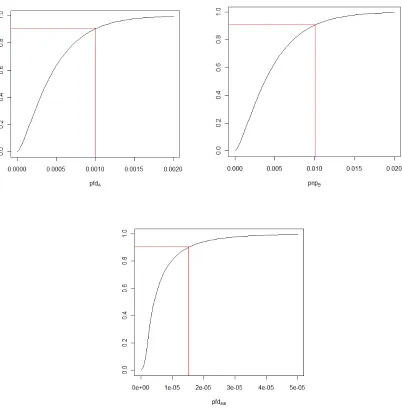
Figure 4 An example where the marginal distributions for pfdA and pnpB in the

first two plots are respectively Beta(1.5, 3150) and Beta(1.5, 315). The third plot shows the resulting conservative (bounding) distribution for the system pfd.

In the case where the marginal distributions are continuous, the function

αA(pA)+αB(t/pA)

has a stationary point at pA = pA *

satisfying the equation

(p_A* )2

⋅α'_A(p_A*

[image:18.612.109.511.144.564.2]

and using this for all t we can obtain a bounding continuous distribution for pfdsys. Alternatively this can be found by numerical optimization.

One way this result might be used is to take a particular level of doubt and propagate claims with this same fixed doubt throughout a case, or part of a case:

Example 7

Figure 4 shows a case where both of the marginal distributions for the parameters are Betas. In the Figure we show the percentiles corresponding to a doubt of 10% for each of the three distributions (the choice of 10% is purely for illustration – it is not intended to represent a realistic figure for real cases). At this level of doubt, claims of 1.0e-03 and 1.0e-02 for pfdA and pnpB allow a claim of approximately 1.5e-05 to be made for the system pfd, and this is, of course, conservative. Readers may think that this near-product of the claims (1.5e-05 versus 1.0e-05), for the fixed 10% doubt, is rather a tight bound.

Example 8

Because complete marginal distributions for the parameters, and the distribution of the system pfd, are known in this case, it follows that the corresponding means are known: E(pfdA) = 0.000476, E(pnpB) = 0.00474

and

E(pfdsys) = 6.97e-06

This compares favourably with the (unattainable) “perfect independence” case: E(pfdA). E(pnpB) = 2.26e-06.

In fact, the Cauchy-Schwarz bound in this case, (15), is 3.75e-06 and is even tighter. However, the point of this approach, via a bounding distribution, is that it allows all bounding percentiles of the system pfd to be computed, not merely the mean.

4

Discussion

reliability is very high – as is the case for some safety-critical systems – this is infeasible (Butler and Finelli 1993; Littlewood and Strigini 1993).

This presents us with an impasse. Whilst there is plentiful evidence that the multi-version approach is effective, at least in some average sense, in achieving high reliability, we cannot usually assess the reliability of a particular diverse system. Such assessment does seem essential, of course, when these systems are critical and their failure may involve the loss of life.

These problems of dependence concern aleatory uncertainty, i.e. uncertainty “in the world” about the failure behaviour of the different channels. The problems are compounded when epistemic uncertainty (uncertainty “about the world”) is also taken into account. So, for a 1-out-of-2 system we would not know the channel pfds with certainty, and, more importantly (and more problematically), there would be uncertainty about the dependence between the channel failure processes. Furthermore, there would be dependencies between these different epistemic uncertainties as well: for example, an assessor’s epistemic beliefs about the value of pfdA would usually be affected by his knowing the size of pfdB.

Clearly, to assess the reliability or safety of a fault tolerant system – for example, for use in a wider system safety case – both aleatory and epistemic uncertainty need to be taken into account. Assessment of channel pfds is relatively straightforward (although it may be very costly). Quite simple statistical analysis from operational testing will allow estimates of individual channel pfds to be obtained, together with confidence bounds that are one way of quantifying epistemic uncertainty. Much more difficult, however, is the problem of expressing jointly an assessor’s uncertainty about two pfds and their dependence, when (as seems likely) these three are not independent.

The work reported here continues our earlier research on these problems. In particular, it extends earlier work so that conservative assessments of system reliability can be obtained without the need to understand any of the dependencies described above.

In the LR work, it was shown how to avoid these problems at the aleatory level. We showed that, for a 1-out-of-2 system in which one channel is possibly perfect, the system pfd is bounded above by the simple product of pfdA and pnpB: that is, the (presumed) aleatory dependence between failures of the channels is not required to be known. The result may be very pessimistic (compared, for example, with an estimate of the system pfd obtained from black-box estimation following massive real-life operational exposure).

It seems likely that this approach will be very conservative: the system pfd can never be better than C. In addition, C seems very difficult to reason about – at least to produce a convincing numerical estimate.

We have presented here two alternatives to the original treatment of epistemic uncertainty in (Littlewood and Rushby 2011). In each case, knowledge of epistemic dependence is not required: the (conservative) results depend only on the two marginal distributions of (i.e. assessor beliefs about) the parameters.

The first approach, in Section 2, obtains bounds as in LR on system pfd – or, more precisely, on the assessor’s posterior mean pfd. The different bounds are based upon different representations of the assessor’s beliefs about the parameters – i.e. what he knows, or is prepared to declare. The first bound is a function only of the four numbers that define a single percentile of the assessor’s beliefs about pfdA and a percentile of pnpB. This bound turns out to be very conservative: it is dominated by the smallest channel “doubt”, αA, and so is rather similar to the LR result in which the “independence doubt”, C, plays a similar role. We therefore considered a refinement in which the assessor is prepared, in addition, to provide for each parameter an upper bound which he believes the parameter cannot exceed. This second bound, not surprisingly, turns out to be less conservative. The third bound requires knowledge of the first two moments of the assessor’s marginal distributions for the parameters. Finally, the fourth bound involves both means and percentiles of the assessor’s marginal distributions for the parameters. We presented illustrative numerical examples for the different bounds. We might expect that the more the assessor knows about the channels, the stronger the claims he can make about the system. This seems to be the case here, where the bounds arising from Theorem 4 involve both means and percentiles and seem to be tighter than the earlier ones.

In our second approach to epistemic uncertainty we obtain a conservative confidence bound for the system pfd. This takes a particularly simple form in the case where the assessor provides only a single percentile for the distribution of each parameter: for an assessor’s channel percentiles in (claim, doubt) form, i.e. (pfdA,αΑ), (pnpB,αΒ), the system pfd is smaller than the product of the channel claims, with doubt equal to the sum of the channel doubts. We generalize this result to the case where the assessor can provide multiple percentiles for the two marginal distributions, and finally to the case where he has a complete distribution for each parameter, for which we obtain a bounding distribution for the system pfd.

Some of these new results are, we believe, better than those arising from the epistemic analysis in (Littlewood and Rushby 2011). Most importantly, they seem likely to be easier to obtain in practice because of the difficulties in arriving at a value for C in that work. That is because the results here avoid completely the difficult problems of estimating dependence, either at the aleatory or at the epistemic levels.

the results in Section 2 concern only a conservative value for the mean of this distribution: this is the number that the assessor might use in answer to the question “what is the pfd of this system?” and be confident that his answer was conservative. The results of Section 3, in contrast concern, in their simplest form, a single point on the right tail of the distribution of the system pfd (via a conservative estimate of a percentile). The more general results provide several conservative percentiles, and in their most general form a complete conservative distribution.

We think there is a tentative case to be made that this confidence bound, or bounding distribution, approach of Section 3 may be less conservative in some useful sense that is worth further study. Being able to make a system claim that is the product of the channel claims, at a price “only” of the sum of the channel doubts seems attractive. For example, consider an assessor who is “happy” to make claims at channel level with 1% doubt. It seems reasonable that he would be “quite happy” with a claim at system level with 2% doubt. If so, he has a strong claim at system level, namely the product of the channel claims, according to the simplest result of Section 3.

Of course, choice between the two approaches is likely to depend upon how the results will be used, and in particular upon the demands of a wider safety case for which claims about the present 1-out-of-2 system (e.g. a protection system) are only a part. The motivation in the original LR work for obtaining a bound for the assessor’s posterior expected system pfd (as we have done here in Section 2) was that, for a Bayesian assessor, this is his system probability of failure on demand. It is the number he would give in answer to the question: “What is the probability that the system will fail on a randomly selected demand?” However there are some subtleties here that provide pitfalls for the unwary. For example, the answer to the question “What is the probability that the system will survive the n demands it will experience in its lifetime?” is not a simple function of the posterior expected system pfd of section 2. That is:

E (1−pfd_sys)n

(

)

≠

₍

1−E(pfd_sys)

₎

n

It follows that the results of Section 2 do not provide an answer to this question, and other similar ones, directly.

A different view is that the assessor is uncertain about the system pfd – his uncertainty being represented by his posterior distribution for this – and so he should propagate this uncertainty through the wider plant safety case (alongside, for example, uncertainties associated with other subsystems), so that any top-level plant claim will have an associated confidence. This is more in the spirit of the results of Section 3. However, it should be noted that such propagation of “complete” uncertainty throughout a complex wider case could be very difficult.

systems (e.g. some protection systems, e.g. some architectures in which the second channel is a simple monitor).

Acknowledgements

Support for the work reported here came from:

• the INDEED project, funded by EPSRC;

• the UnCoDe project, funded by the Leverhulme Trust;

• the DISPO project, funded under the CINIF Nuclear Research Programme by EDF Energy Limited, Nuclear Decommissioning Authority (Sellafield Ltd, Magnox Ltd), AWE plc and Urenco UK Ltd. (“the Parties”). The views expressed in this Report are those of the author(s) and do not necessarily represent the views of the members of the Parties. The Parties do not accept liability for any damage or loss incurred as a result of the information contained in this Report.

References

Bishop, P., R. Bloomfield, et al. (2011). "Towards a formalism for conservative claims about the dependability of software-based systems." IEEE Trans Software Engineering

35(5): 708-717.

Boeing (2010). Statistical Summary of Commercial Airplane Accidents, Worldwide Operations, 1959-2009. Seattle, Aviation Safety, Boeing Commercial Airplanes.

Butler, R. W. and G. B. Finelli (1993). "The infeasibility of quantifying the reliability of life-critical real-time software." IEEE Trans Software Engineering 19(1): 3-12.

Eckhardt, D. E., A. K. Caglayan, et al. (1991). "An experimental evaluation of software redundancy as a strategy for improving reliability." IEEE Trans Software Eng 17(7): 692-702.

Eckhardt, D. E. and L. D. Lee (1985). "A Theoretical Basis of Multiversion Software Subject to Coincident Errors." IEEE Trans. on Software Engineering 11: 1511-1517. FAA (1988). Advisory Circular 25.1309-1A: System design and analysis. Washington DC, Federal Aviation Administration.

Knight, J. C. and N. G. Leveson (1986). "Experimental evaluation of the assumption of independence in multiversion software." IEEE Trans Software Engineering 12(1): 96-109.

Kruskal, W. (1988). "Miracles and Statistics: The Casual Assumption of Independence." Journal of the American Statistical Association 83(404): 929-940.

Littlewood, B. and J. Rushby (2011). "Reasoning about the reliability of diverse two-channel systems in which one two-channel is 'possibly perfect'." IEEE Trans Software Engineering.

Littlewood, B. and L. Strigini (1993). "Validation of ultra-high dependability for software-based systems." CACM 36(11): 69-80.

Littlewood, B. and D. Wright (1997). "Some conservative stopping rules for the operational testing of safety-critical software." IEEE Trans Software Engineering 23(11): 673-683.

Littlewood, B. and D. Wright (2007). "The use of multi-legged arguments to increase confidence in safety claims for software-based systems: a study based on a BBN of an idealised example." IEEE Trans Software Engineering 33(5): 347-365.

May, J., G. Hughes, et al. (1995). "Reliability estimation from appropriate testing of plant protection software." Software Engineering Journal 10(6): 206-218.

Rouquet, J. C. and P. J. Traverse (1986). Safe and reliable computing on board the Airbus and ATR aircraft. Safecomp: 5th IFAC Workshop on Safety of Computer Control Systems, Pergamon Press.

RTCA (1992). Software considerations in airborne systems and equipment certification, DO-178B, Requirements and Technical Concepts for Aeronautics.

Appendix

Lemma: If

0≤X≤1, and P(X>p)=α, and E(X)≤p, then

E(X2)≤E(X)

2

α ≤

p2

α

Proof:

Let E(X)=m and E(X2 )=s2

We show that there exists a two-point discrete random variable, Y, as follows:

P(Y =y)=1−α

P(Y =z)=α where

0≤y≤m≤z≤1

and

E(Y)=y×(1−α)+z×α=m E(Y2

)=y2

×(1−α)+z2

×α=s2 (A1)

From (A1) we have y=m−z×α 1−α and

E(X2

)=E(Y2

)=G(z)=(m−z×α)

2

1−α +z

2

α

If α>0 the equation G(z)=s2

has a positive real root:

z=m+ (s2−m2)×1−α

α

since s2 −m2

=Var(X)≥0.

It follows that the random variable Y always exists. Now, if z>0, then G(z) is increasing because

dG(z) dz =−

2α(m−z×α)

1−α +2zα=

−2mα+2α2z+2αz−2α2z

1−α =

2α(z−m) 1−α ≥0; and

therefore

E(X2

)=E(Y2 )≤m2

/α=E(X)2

/α≤p2 /α

that is

E(X2

)≤E(X) 2

α ≤

p2 α