Testing a linear ARMA Model against threshold-ARMA models : a Bayesian approach

Testing a Linear ARMA Model against

Threshold-ARMA Models: a Bayesian Approach

R

ubing

L

iang

Q

iang

X

ia

J

iazhu

P

an

J

inshan

L

iu

a_{College of Science, South China Agricultural University, Guangzhou 510642, P.R. China} b_{Department of Mathematics and Statistics, University of Strathclyde, Glasgow G1 1XH, UK}

Abstract. We introduce a Bayesian approach to test linear autoregressive

moving-average (ARMA) models against threshold autoregressive moving-moving-average (TARMA)

models. Firstly, the marginal posterior densities of all parameters, including the

thresh-old and delay, of a TARMA model are obtained by using Gibbs sampler with

Metropolis-Hastings algorithm. Secondly, reversible-jump Markov chain Monte Carlo (RJMCMC)

method is adopted to calculate the posterior probabilities for ARMA and TARMA

mod-els: Posterior evidence in favor of TARMA models indicates threshold nonlinearity.

Fi-nally, based on RJMCMC scheme and Akaike information criterion (AIC) or Bayesian

information criterion (BIC), the procedure for modeling TARMA models is exploited.

Simulation experiments and a real data example show that our method works well for

distinguishing a ARMA from a TARMA model and for building TARMA models.

Mathematics Subject Classification (2010) : 62F10, 62F15

Key words: Bayesian inference; ARMA models; Gibbs sampler; Metropolis-Hastings

algorithm; RJMCMC methods; AIC; BIC; TARMA models.

∗_{Corresponding author, E-mail: [email protected]}

1

Introduction

Threshold autoregressive (TAR) models have become a standard and popular class of nonlinear

time series models to describe the asymmetric phenomena in many branches of science and social

science. Since Tong (1978) and Tong and Lim (1980), a huge amount of literature on theoretical

properties and statistical inference of TAR models has appeared, see Tong (1990) and Tsay (2005)

among others. But complicated analytical works and numerical multiple integration is involved

in statistical inference of TAR models by the likelihood approaches. To overcome the computing

problem and to avoid analytical difficulty, some authors have applied Bayesian method to carry out

parameter estimation for TAR models. Mcculloch and Tsay (1993a, 1993b) proposed a Bayesian

procedure for detecting threshold values in a TAR model via posterior probability plots. Chen and

Lee (1995) applied the Gibbs sampler of Geman and Geman (1984), and the Metropolis-Hastings

(M-H) algorithm of Metropolis et al. (1953) and Hastings (1970), for inference of TAR models. So

and Chen (2003) developed an efficient way to select the best subset from threshold autoregressive

models.

Some authors have realized that threshold moving average (TMA) models have their own

ad-vantages and are as important as TAR models in practice, see Ismail and Charif (2003) and Ling

and Tong (2005) among others. Ismail and Charif (2003) introduced a Bayesian analysis for TMA

models, and Ling and Tong (2005) proposed a likelihood ratio test for linear MA model against

TMA models. Recently, Xia et al. (2010) gave Bayesian test for nonlinear of a TMA model.

However, in order to get a parsimonious model for asymmetrical high order dependence, some

authors found that threshold autoregressive moving average (TARMA) should be used. For

like-lihood approach to statistical inference of TARMA models, analytical works and computation are

even more complicated than those for TAR and TMA models. So Bayesian method has been used

to do statistical analysis of TARMA models, see for instance S´afadi and Morettin (2000), Chen,

Liu and Gerlach (2011), and Xia et al. (2012). Chen et al. (2011) developed an efficient way

to select a subset from a general family of TARMA models, but they did not give any discussion

about the threshold nonlinear test. Meanwhile, fundamental theory about TARMA models, such

as identifying the threshold and delay values, estimating the parameters, and testing the threshold

nonlinearity, needs to be developed further.

The aim of this paper is to propose a Bayesian test for the threshold nonlinearity of TARMA

models. Firstly, Bayesian estimation of the threshold value and other parameters of TARMA

mod-els is investigated. Chen and Lee (1995) and S´afadi and Morettin (2000) adopted the MCMC

technique and used the arranged autoregression approach to estimate the threshold and delay

val-ues as well as the coefficients simultaneously. Basing on their work, we combine Gibbs sampler

and Metropolis-Hastings algorithm to give a Bayesian analysis of two-regime TARMA models.

We do not need to employ the arranged autoregression. Secondly, to avoid analytical difficulty and

complicated computation, Xia et al. (2010) applied the RJMCMC method (Green, 1995) for

test-ing TMA models, but they only constructed kernels by not includtest-ing the variance parameter. We

know that the variance parameter, especially different variance in each regime, is a very important

characteristic for the TARMA models to be identified. Thus, we add the variance parameter into

the kernels by using the reversible-jump MCMC method for testing TARMA models. It is

demon-strated that the reversible-jump method is easy to implement and fits well within our framework of

Bayesian procedure. Finally, since the order of each regime is also important to TARMA models,

we will try to combine the reversible-jump MCMC method and AIC or BIC to determine whether

the threshold nonlinearity is significant.

The context of this paper is arranged as follows. The TARMA models and the methodology

of Bayesian inference are presented in Section 2. Section 3 gives details of a Bayesian model

selection procedure by RJMCMC method. Section 4 exploits the procedure for modeling TARMA

models briefly. Simulation results and a real data example are presented in Section 5. Section 6 is

our conclusion.

Throughout the paper, we denote the transpose of a matrix A by A0.

2

Threshold ARMA and Its Bayesian Inference

2.1

TARMA Model

A time series{Yt,t=1,2, ...}is said to follow a TARMA(2; p1,q1,p2,q2,d) model with two regimes

if it satisfies the following equation

Yt =

    

φ(1)₀ +

p1

P

j=1

φ(1)_j Yt−j+

q1

P

k=1

θ(1)_k ξ_t(1)_−k +ξ(1)_t , Yt−d > r

φ(2)₀ +

p2

P

j=1

φ(2)_j Yt−j+

q2

P

k=1

θ(2)_k ξ_t(2)_−k +ξ(2)_t , Yt−d ≤ r

(2.1.1)

where{ξ_t(i)_}is assumed to be a sequence of independent and identically distributed (i.i.d.) random

variables with common distribution N(0, σ2

i), p1,q1,p2,q2,d are positive integers. Here d is called

the delay (or threshold lag) parameter of the model, and r∈R is called the threshold parameter.

2.2

Bayesian Inference

Suppose we have a sample Y= {Y1,Y2, ...,Yn}. Let p= max{p1,p2}and q =max{q1,q2}. Then we

assume the threshold variable Yt−dtakes values in{Yh−d, ...,Yn−d}, where h=max{d+1,p+1,q+1}.

Given the first h−1 observations and ξ₁(i) = ... = ξ_h(i)₋₁ = 0, the conditional likelihood function of

TARMA(2; p1,q1,p2,q2,d) model can be easily obtained as follows

L(Φ1,Φ2, σ21, σ 2

2,r,d |Y)

∝σs1

1σ s2 2 exp ( − 1 2σ2 1 n P

t=h

Yt −φ(1)₀ −φ(1)₁ Yt−1−...−φ(1)p1Yt−p1

−θ(1)₁ ξ(1)_t−1−...₋θ(1)q1ξ

(1)

t−q1

2

I(Yt−d >r)

− 1

2σ2 2

n

P

t=h

Yt−φ(2)₀ −φ(2)₁ Yt−1−...−φ(2)p2Yt−p2

−θ(2)

1 ξ

(2)

t−1−...−θ (2)

q2ξ

(2)

t−q2

2

I(Yt−d ≤r)

)

(2.2.1)

where I is the indicator function, and s1 = P

t=h

I(Yt−d >r),s2 = P

t=h

I(Yt−d ≤r). Denote

Y = Yh,Yh+1, ...,Yn0, Ξ1 = ξ(1)_h , ξ_h(1)₊₁, ..., ξn(1)

0_{, Ξ}

2 = ξ_h(2), ξ(2)_h+1, ..., ξn(2)

0_,

Φ1 = φ(1)₀ , φ(1)₁ , ..., φ(1)p1, θ

(1)

1 , ..., θ

(1)

q1

0_{, Φ}

2 = φ(2)₀ , φ(2)₁ , ..., φ(2)p2, θ

(2)

1 , ..., θ

(2)

q2

0_,

I1 = diag

I(Yh−d >r), I(Yh+1−d > r), ..., I(Yn−d > r)

,

I2 = diag

I(Yh−d ≤r), I(Yh+1−d ≤ r), ... ,I(Yn−d ≤ r)

,

X1 =       

1 Yh−1 ... Yh−p1 ξ

(1)

h−1 ... ξ (1)

h−q1

1 Yh ... Yh+1−p1 ξ

(1)

h ... ξ

(1)

h+1−q1

.. .. .. .. .. .. ..

1 Yn−1 ... Yn−p1 ξ

(1)

n−1 ... ξ (1)

n−q1

       , and

X2 =       

1 Yh−1 ... Yh−p2 ξ

(2)

h−1 ... ξ (2)

h−q2

1 Yh ... Yh+1−p2 ξ

(2)

h ... ξ

(2)

h+1−q2

.. .. .. .. .. .. ..

1 Yn−1 ... Yn−p2 ξ

(2)

n−1 ... ξ (2)

n−q2

       . Then

Ξ1 = I1 Y −X1Φ1), Ξ2 = I2(Y −X2Φ2,

and we can rewrite (2.2.1) as

L(Φ1,Φ2, σ2₁, σ₂2,r,d |Y)∝ |Σ1|−

1 2|Σ

2|−

1

2 ∙exp− 1

2(Ξ01Σ− 1

1 Ξ1+ Ξ02Σ− 1 2 Ξ2)

_(2.2.2)

where Σ1 = diag σ2₁, ..., σ2₁ and Σ2 = diag σ2₂, ..., σ2₂ are all (n−h+1)× (n− h+ 1) diagonal

matrix, respectively. Taking{ξ_t(i) =0,t<h}, we can compute{ξ(i)_t ,t≥ h}recursively as follows

ξ(1)_t =Yt −X1t0 Φ1 if Yt−d >r; ξt(2)= Yt−X02tΦ2 otherwise, (2.2.3)

where X1t = 1,Yt−1, ...,Yt−p1, ξt−1, ..., ξt−q1 , X2t = 1,Yt−1, ...,Yt−p2, ξt−1, ..., ξt−q2 .

To carry out the Bayesian inference about the parametersΦ1,Φ2, σ2₁, σ2₂,r,d in the TARMA(2; p1,

q1,p2,q2,d) model, we need to obtain the marginal distribution by the joint posterior distribution

P(Φ1,Φ2, σ2₁, σ2₂,r,d|Y), which is difficult to be finished and can be replaced by using conditional

posterior distributions in a MCMC process. Therefore, we need to choose priors to derive the

conditional posterior distribution for the unknown parameters.

Referring to Chen and Lee (1995), Xia et al. (2010), and Chen et al. (2011) we assume that

Φi follows N(Φ0i,Vi−1), where Videnotes the precision, i = 1,2, andΦ1 is independent ofΦ2. Let

σ2

i follow the inverse gamma distribution IG(αi, βi), where the hyper-parameters are known. For r,

similar to Geweke and Terui (1993), we adopt that it follows a uniform distribution on an interval

(a,b). Assume that d follows a discrete uniform distribution on a set of integers{1,2, ...,d0}, where

d0is a prescribed positive integer.

Using Bayesian techniques, we derive the conditional posterior distributions ofΦ1,Φ2, σ2₁, σ2₂,r,d

based on the above priors as follows.

(1) The conditional posterior probability function ofΦiis

p(Φi |Y, σ2₁, σ2₂,r,d) ∝exp

(

− 1

2

Ξ0_iΣ−1

i Ξi+

Φi−Φ0i 0

Vi

Φi−Φ0i )

(2.2.4)

for i= 1,2.

(2) The conditional posterior distribution ofσ2

i is

p(σ2

i |Y,Φ1,Φ2,r,d)∼ IG αi +

si 2, βi+

S2_i

2

_{, (2.2.5)}

where S2_i = Ξ0_iΞi for i=1,2.

(3) The conditional posterior probability function of r is

p(r |Y,Φ1,Φ2, σ2i, σ

2

2,d)∝ exp

h

− 1₂S

2 1 σ2 1 + S 2 2 σ2 2 i

∙I(a< r< b). (2.2.6)

Note that S_i is a function of r.

(4) The conditional posterior probability function of d is a multinomial distribution with

proba-bility

p(d |Y,Φ1,Φ2, σ21, σ 2 2,r)=

L(Φ1,Φ2, σ2₁, σ2₂,r,d|Y)

d0

P

d=1

L(Φ1,Φ2, σ2₁, σ2₂,r,d |Y)

(2.2.7)

where d =1,2, ...,d0.

2.3

Sampling Scheme

From the previous section, we see that the conditional densities for σ2

i and d can be identified.

Then, the Gibbs sampler can be used. But there are not closed form for the conditional distributions

of r andΦi (i = 1,2). The random walk Metropolis-Hastings (M-H) algorithm will be applied to

draw Φi, i = 1,2, and r. Details of the Gibbs sampler and Metropolis-Hastings algorithm can

be found in Casella and George (1992) and Chib and Greenberg (1995), respectively. Denote the

target density in (2.2.3) by f1(∙). The algorithm for drawingΦi is described below.

Step 1: At iteration j, generate a pointΦi from the random walk kernel

Φi = Φ[ j_i −1]+ξΦi, ξΦi ∼ N(0,Σ

∗

Φi)

whereΦ[ j_i −1]is the ( j−1)th iterate forΦi.

Step 2: AcceptΦi asΦ[ j]_i with probability p = min{1, f1(Φi)/f1(Φ_i[ j−1])} > u,u ∼

U(0,1). Otherwise, setΦ[ j]_i = Φ[ j_i −1].

We usually selectΣ∗_Φ

i to be a diagonal matrix, whose elements are tuned by monitoring the

accep-tance rate between 0.25 and 0.75.

Remark 1. Chen et al. (2011) employed the modified GM (George and McCulloch, 1993)

method for M-H steps ofΦi, we use the similar idea to drawΦi.

Denote the target density in (2.2.5) by f2(∙). The algorithm for drawing r is described as follows.

• At iteration j, generate a point r from the random walk kernel

r =r[ j−1]+ξr, ξr ∼ N(0, σ∗r

2

)

where r[ j−1]_{is the ( j−1)th iterate of r.}

• Accept r as r[ j] with probability p= min{1, f2(r)/f2(r[ j−1])}> u,u ∼ U(0,1).

Otherwise, set r[ j] _=r[ j−1]_.

In summary, we use the following iterative sampling scheme to construct the desired posterior

sample:

(1) DrawΦi using the random walk Metropolis-Hastings algorithm from the conditional

poste-rior distribution in (2.2.3), i= 1,2;

(2) Drawσ2

i from the inverse Gamma distribution in (2.2.4), i=1,2;

(3) Draw r using the random walk Metropolis-Hastings algorithm the conditional posterior

dis-tribution in (2.2.5);

(4) Draw d from a multinomial distribution with probabilities proportional to the likelihood

func-tion in (2.2.6).

This completes one iteration. Of course, we can change the order in sampling the variables. So

and Chen (2003) have illustrated that fast convergence is attained irrespective of the order. In

addition, these desired posterior samples will be used in RJMCMC scheme to test the significance

of threshold nonlinearity by comparing a ARMA model and its counterpart of a TARMA model,

and the details are introduced in the following section.

Remark 2. Chen et al. (2011) pointed out that it remains difficult to find necessary and

suf-ficient conditions of stationarity and invertibility for the general TARMA model. Therefore, we

simply ignore the stationary assumptions and proceed to use the normal-gamma family as a

con-jugate prior distribution, such as in Chen (1999), So and Chen (2003) and So et al. (2006) for AR,

TAR and ARX-GARCH models, respectively.

3

Selecting Model by RJMCMC

The main goal of our study is to test for the threshold nonlinearity of TARMA models. The testing

problem will be transferred to a Bayesian model-selection problem. To do this, we need to calculate

the posterior probabilities P(Mk|Y),k = 1,2, where M1 and M2 represent ARMA and TARMA

models respectively. The RJMCMC method in Green (1995), which is a very useful mechanism

to allow jumps between spaces with different dimensions while maintaining the detailed balance

condition ensuring convergence of the Markov chain, can be adopted here. This method was used

to choose between pairs of GARCH models by Vrontos et al. (2000), So et al. (2005), Chen et al.

(2008).

We consider the jump from M1 with parameter Φ(1) to M2 with parameter Φ(2). Here Φ(1)

consists of a set of ARMA parameters, and Φ(2) consists of Φ1, Φ2, σ2₁, σ2₂ and r in TARMA

model. Generally speaking,Φ(1) andΦ(2)have different dimensions. To jump from M1to M2, we

construct two variables U(1)_{and U}(2)_{to form a bijection between (Φ}(1)_,U(1)_{) and (Φ}(2)_,U(2)_{), that is,}

an one-to-one bijective transformation which links (Φ(2)_,U(2)_{) with (Φ}(1)_,U(1)_{). This transformation}

ensures the necessary condition that the dimensions of (Φ(1)_,U(1)_{) and (Φ}(2)_,U(2)_{) are the same, i.e.,}

dim(Φ(1)_)+dim(U(1)_)=dim(Φ(2)_)+dim(U(2)_).

To jump from M1to M2, we simulate U(1)from a kernel Q1(U(1)|Φ(1)) and determineΦ(2)from

Q2(U(2)|Φ(2)). Then, we accept the jump with probability min{1,p}, where

p= L(Y|M2,Φ

(2)_)Π(Φ(2)_|M

2)P(M2)J(M1,M2)Q2(U(2)|Φ(2)) L(Y|M1,Φ(1))Π(Φ(1)|M1)P(M1)J(M2,M1)Q1(U(1)|Φ(1))∙

∂(Φ

(2)_,U(2)₎

∂(Φ(1)_,U(1)₎

. (3.1)

The term L(Y|Mi,Φ(i)) is the likelihood function of model Mi, Π(Φ(i)|Mi) is the prior distribution,

and P(Mi) is the prior probability, i = 1,2. Denote the probability of the jump from Mi to Mj by

J(Mi,Mj). The last part in (3.1) is the Jacobian of the transformation. We can implement the jump

from M2to M1in the reversed way by simulating U(2)from a kernel Q2(U(2)|Φ(2)) and determining

Φ(1)from Q1(U(1)|Φ(1)) to calculate the acceptance probability min{1,p−1}.

To introduce the bijection for RJMCMC, we follow Vrontos et al. (2000), So et al. (2005),

and define U(1) = Φ(2), U(2) = Φ(1), which implies a Jacobian_∂(Φ∂(Φ(2)(1)_,,U_U(2)(1))₎ = 1. In addition, we set

J(Mi,Mj)=1 to allow a jump in each MCMC iteration, and P(M1) =P(M2)=0.5 to reflect prior

model ignorance. In this case, we can simplify the acceptance probability of reversible jump in

(3.1) to

p= L(Y|M2,Φ

(2)_)Π(Φ(2)_|M

2)Q2(U(2)) L(Y|M1,Φ(1))Π(Φ(1)|M1)Q1(U(1))

(3.2)

with the kernels Q1 and Q2 being independent ofΦ(1)andΦ(2), respectively.

It is important to choose appropriate kernels Q1 and Q2 to apply the RJMCMC successfully.

To do this, firstly, the Gibbs sampler combining with random walk M-H algorithm in the

subsec-tion 2.3 is implemented for M iterates, and sample means μΦi, μr, μσ2_i, μd, the sample covariance

matrix ΣΦi and sample variances σ

2

r, σ2_σ2

i

, σ2

d can be obtained. And then, we will substitute μd

for d in the TARMA model, and use μΦi,ΣΦi, μr, σ

2

r and μσ2

i,Σσ

2

i to form the Gaussian kernels

N(μΦi,ΣΦi),N(μr, σ

2

r) and N(μσ2

i,Σσ

2

i)I(σ

2

i > 0). Therefore, we select the kernel Q1(U

(1)_{) for}

draw-ingΦ(2) _{= (Φ}0

1,Φ02,r, σ 2 1, σ

2

2)0 to be the product of the above four Gaussian kernels, i.e., Q1(U

(1)_)∼

N(μΦ1,ΣΦ1)∙N(μΦ2,ΣΦ2)∙N(μr, σ

2

r)∙N(μσ2,Σσ2 1)I(σ

2

1 > 0)∙N(μσ22,Σσ22)I(σ

2

2 >0). For the

simula-tion of u(2), which is the parametersΦ(1) = ( ˜Φ0, ˜σ2₎0_{in ARMA model, we use the same method as}

described in the previous section to construct N(μ_Φ˜,Σ_Φ˜) and N(μσ˜2,Σ_σ˜2)I( ˜σ2 >0) from the first M

iterates of ˜Φand ˜σ2_{. We then choose Q}

2(u(2))∼ N(μ_Φ˜,Σ_Φ˜) N(μσ˜2,Σ_σ˜2)I( ˜σ2 > 0) as the kernel for

drawingΦ(1)=( ˜Φ0,σ˜2₎0_{. In summary, the jumping scheme is as follows.}

• From ARMA(M1) to TARMA (M2):

(1) DrawΦi ∼N(μΦi,ΣΦi),i=1,2, r∼ N(μr, σ

2

r) andσ2i ∼ N(μσ2

i,Σσ

2

i)I(σ

2

i >

0) and accept the jump with probability min{1,p}.

(2) If accepted, updateΦ(2)_{. Otherwise, updateΦ}(1)_.

• From TARMA(M2) to ARMA (M1):

(1) Draw ˜Φ ∼ N(μ_Φ˜,Σ_Φ˜), ˜σ2 ∼ N(μσ˜2,Σ_σ˜2)I( ˜σ2 > 0), and accept the jump

with probability min{1,p−1_}.

(2) If accepted, updateΦ(1). Otherwise, updateΦ(2).

4

Modeling TARMA Models

Based on the results of RJMCMC method, we propose a procedure for building a TARMA model,

as long as its threshold nonlinearity is significant. We hope that the potential of TARMA models

can be exploited by this procedure in simulation and application, which consists of several steps

and is described as follows.

Step 1. Select the appropriate AR order p and MA order q for ARMA models by AIC or BIC.

Step 2. For given p and q, use the sampling scheme as described in Subsection 2.3 to construct

the Gaussian kernels (N(μΦ˜,ΣΦ˜),N(μσ˜2,Σ_σ˜2)I( ˜σ2> 0)) for ARMA model.

Step 3. For given p and q, use the sampling scheme as described in Subsection 2.3 to construct

the Gaussian kernels (N(μΦ1,ΣΦ1), N(μΦ2,ΣΦ2), N(μr, σ

2

r), N(μσ2 1,Σσ

2 1)I(σ

2

1 >0), N(μσ22,Σσ 2 2)I(σ

2 2 >

0)) for TARMA model.

Step 4. Using the jumping scheme, choose the appropriate TARMA model. If necessary, refine

the AR order, MA order and parameters of TARMA model with AIC or BIC and MCMC sampling

scheme again.

Remark 3. For the specified ARMA or TARMA model, the AIC and BIC are taken as the

following form

AIC(k)= −ln(L)+2k, BIC(k)= −ln(L)+ln(n)k

where L is the likelihood value for the model in (2.1.1), n is the ”effective number of observations”

and k is the number of independent parameters of the models.

5

Simulation Experiments and a Real Data Example

In this section, we first present simulation results to show the effectiveness of our MCMC sampling

scheme, model selection method and the procedure for modeling TARMA models, and then apply

our method to a real data set.

5.1

Simulation Experiments

We set M = 8000 in all experiments, and apply the sampler scheme to draw all parameters

and to form the means and the normal kernels by discarding the first 5000 iterations. We then

perform 8000 iterations for posterior inference and model selection. The hyper-parameters are

Θ0i = (0, ...,0)0p+q,Vi = diag(0.1, ...,0.1)p+q, i = 1,2, and furthermore we choose α = 2.5, β =

1.6, d0 = 3, a = p10, b = p90, where p and q is the most AR and MA order of TARMA

model respectively, pk denotes the kth percentile of the data.

The RJMCMC scheme in testing the significance of threshold nonlinearity will be studied

firstly. The null is the ARMA(1,1) model with constant term φ0 = 0, and the alternative is the

TARMA(2; 1,1,1,1,1) model with constant terms φ( j)₀ = 0, j = 1,2,r = 0, φ₁(2) = θ(2)₁ = 0.5

andφ(1)₁ = θ(1)₁ = −1, ₋0.5, 0, 0.2, 0.4, 0.5, denoted by model 1 ∼ 6 respectively. We

generate 400 points of y with y0 = 0, but only use the last 300 observations as data set for each

realization. Table 1 lists the posterior probabilities (prob.) of identifying the true models, the

posterior means, the posterior standard deviations (s.d.) for the true model efficiently.

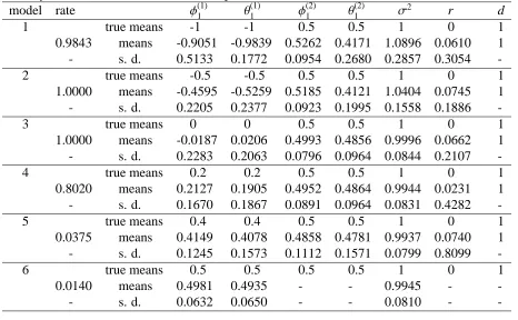
From Table 1, it is clear that the posterior means are closed to the true values under the good

performance of the RJMCMC scheme testing, although there are slightly bias for φ(1)₁ of model 3

and r of model 4 and 5.

To make some discussion about the power of the proposed Bayesian test and the effectiveness

of our MCMC sampling scheme, we continue to study the above models with the same prior setting

as the generated examples before based on 500 samples each with size 300. The rate of correct

selections of TARMA models (rate) and Bayesian estimates of the above six models are shown

in Table 2. From Table 2, our results in this simulation study are fine. Based on 500 samples

each with size 300, the estimates of the coefficients are approximately unbiased, and the power of

correct selections of TARMA models increases when the alternative departs from the linear ARMA

model.

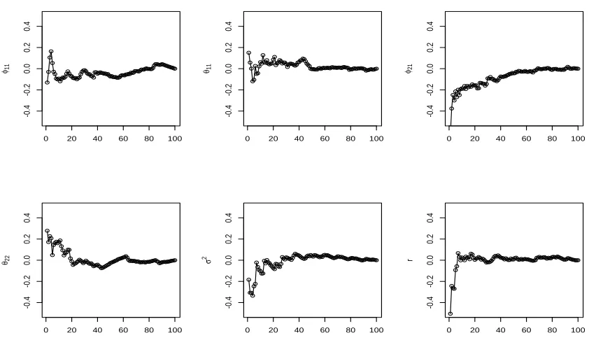
For the check of convergence of our algorithm, we will use the visual inspection of CUMSUM

statistics (Yu and Mykland, 1994) defined by

CSt = 1

t

t

X

j=1

θ( j)_−μ

θ/σθ

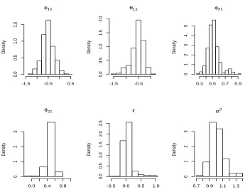
whereμθ andσθ are the empirical mean and standard deviation of the 500 draws. Figure 1 shows

that our algorithm is almost convergent for the model 2 in some sense. Meanwhile, the histogram

of all parameters are nearly symmetric form the Figure 2.

To illustrate the usefulness of our procedure for building a TARMA model a bit further, we

conduct an preliminary investigation about the following two TARMA models. Here, we also

generate 400 points of y with y0 = 0 and discard the first 100 observations as data set for each

realization, and then carry out MCMC iterations for them.

• Model 7: T ARMA(2; 1,1,1,1,1)

Yt =

    

ξt +0.6ξt−1+0.4Yt−1, Yt−1 >0.5

ξt −0.5ξt−1−0.3Yt−1, Yt−1 ≤0.5

ξt ∼ N(0,1).

(5.1)

• Model 8: T ARMA(2; 2,1,3,1,2)

Yt =

    

ξt −0.4ξt−1+0.8Yt−1−0.6Yt−2, Yt−2> −0.1

ξt +0.4ξt−1+0.2Yt−1+0.5Yt−3, Yt−2≤ −0.1

ξt ∼ N(0,1).

(5.2)

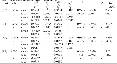
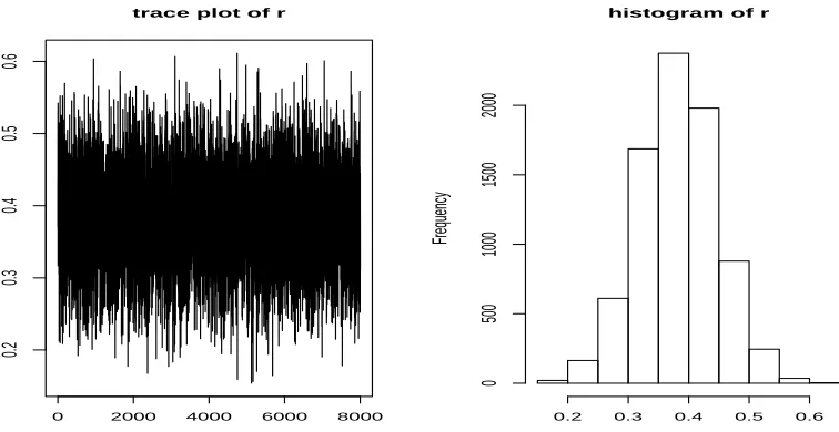
For the data simulated from model 7, we choose (p,q) = (2,2) for ARMA model by AIC or

BIC, and then we investigate the four cases of RJMCMC scheme testing by decreasing the order

(p,q) and obtain the corresponding results recorded in Table 3. Although the true order (p,q) of

model 7 is (1,1), the RJMCMC scheme testing is still efficient and the posterior means are almost

closed to the true values in other cases of appropriate AR and MA order. In particular, the posterior

means of some parameters are quite closed to 0, which is the true values of model 7. Furthermore,

AIC and BIC values indicate that (p,q) = (1,1) is the best choice, which just suggests that our

procedure for building a TARMA model may be useful. In addition, the posterior means of all

parameters, the trace plot and the histogram of r (Figure 1) show that the final modeling results

would pass in crow.

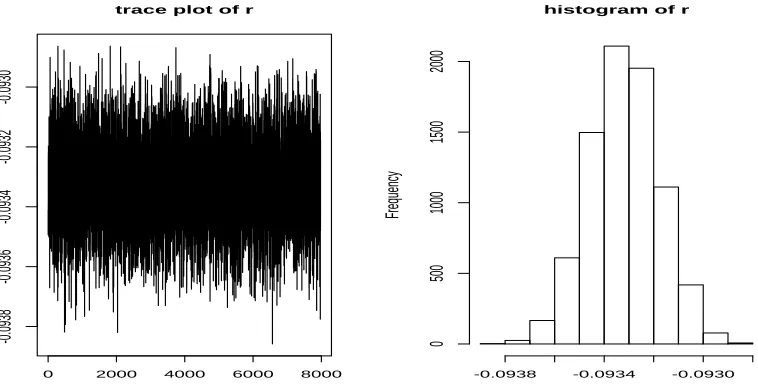
For model 8, this is an special example, we hope our MCMC algorithm to be useful to it by

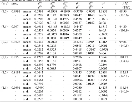
identifying as TARMA(2; 2,1,3,1,2) model with φ(2)₂ = 0. Firstly, we select the order (p,q) =

(3,2) for ARMA model by AIC or BIC. To examine the efficiency of the RJMCMC scheme, we

also attempt to change the order as low as possible. Table 4 lists the results for six cases, which

illustrate that the RJMCMC scheme can obtain good performance on the nonlinear case. If the

order (p,q) of the fitted model is lower than the true model, the values of AIC and BIC will be

larger. Under these circumstances, we should refine the order (p,q) to gain the final results by AIC

and BIC again. If the order (p,q) of the fitted model is larger than or equal to the true model, the

posterior means of parameters are quite closed to the true values as well. The final model may

be TARMA(2; 2,1,3,1,2), which can keep close consistent to model 8, althoughφ(2)₁ andφ(1)₃ has

slightly bias, the other estimates are close to the true parameters, especially theφ(2)₂ is close to 0.

Meanwhile, the trace plot and the histogram of r (Figure 2) also give fine results.

The visual inspection of CUMSUM statistics are also used to check the convergence of our

algorithm to r of model 7 and 8, depicted in Figure 5, which indicates that our MCMC algorithm

has been almost convergent in some sense.

The above simulation analysis shows that our MCMC sampling methods can perform well in

providing posterior samplers for statistical inference for TARMA models. Therefore, it should be

useful in practice.

Remark 4. The maximum of AR and MA order is prescribed to 3 in all above simulations. In

addition, the order p and q can be also chosen starting from the low order.

5.2

Some Real Data Examples

To make a supplement for our MCMC sampling method, we consider a data set in an application:

the exchange rate of Japanese Yen v.s. USA dollar. Similar to Chen and Lee (1995) and Xia et al.

(2010), the hyper-parameters used areΦ0i = (0,0)0 for i = 1,2, V = diag(0.1,0.1), α = 2.5, β =

1.6, and a= p5and b= p95, which are defined as in subsection 5.1. Set M =10000 to run MCMC

iterations. Burning the first 5000 times, the posterior means and variances can be got to form the

normal kernels which are applied to RJMCMC iterations for 10000 times.

The monthly data from Jan. 1971 to Dec. 2000 are used and there are 360 observations. This

data set were analyzed recently by Ling and Tong (2005) and Xia et al. (2010). Pt denotes the

exchange rate at tth month. Let xt = 100[log(Pt)−log(Pt−1)] and yt = xt −

360_P

i=2

xi/359 for t ≥ 2.

We take the order (p,q) = (1,1) for ARMA model by AIC and BIC, i.e., employ ARMA(1,1)

and TARMA(2; 1,1,1,1,d) models to fit the data {y2,y3, ...,y360}. The estimate of the posterior

probability identifying the TARMA model is 0.7813, which suggests that the threshold nonlinearity

is significant. According to our procedure for modeling TARMA model, we should refine the order

(p,q) by AIC or BIC and MCMC sampler. Table 5 lists the values of AIC and BIC, which illustrate

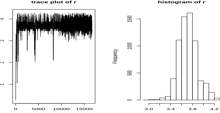
that (p,q)=(1,1) is best choice for TARMA model. For illustrative purposes, we obtain estimated

model (4.1) with the standard errors in the square brackets. From model (4.1), we can see that

the estimates of threshold and delay parameters are r = 3.7197 and d = 3 respectively. Figure 4

displays the trace plot for all MCMC iterations of r and the histogram of r for TARMA model.

We see that the trace plot of r is stationary gradually, and after 5000 MCMC iterations it is almost

stationary. The histogram of r also shows that its distribution is symmetric in some sense.

Yt =

          

−0.9663Yt−1+0.6666ξt−1+ξt,Yt−3 >3.7197

(0.1981) (0.1481) (0.0293)

0.0494Yt−1+0.3863ξt−1+ξt,Yt−3≤ 3.7197

(0.0144) (0.0120)

ξt =

√

6.7239et, et ∼ N(0,1).

(0.0293)

(4.1)

6

Conclusion

In this paper, we develop a Bayesian testing scheme for threshold nonlinearity of two-regime

TARMA models. Firstly, combining Gibbs sampler and Metropolis-Hastings algorithm, we

pro-pose a Bayesian method to analysis the TARMA models. And then, with these Bayesian estiamtes,

we use a RJMCMC algorithm to select model between a ARMA model and a TARMA model by

constructing the Normal kernels. The main idea is to compute the posterior probabilities of

com-petitive models, hence, our procedure can avoid some analytical difficulty and complicated

compu-tation, therefore, it is simple to implement and requires no subjective specification of threshold and

delay values. This is the main advantage of our Bayesian approach. Finally, based on RJMCMC

scheme and AIC or BIC, we give the procedure for modeling TARMA models. Simulation results

and a real data example show that our approach can perform good. However, this work is only

limited to two-regime case without considering the heteroscedastic model. In the further research,

the heteroscedasticity can be added as an extension of our work.

ACKNOWLEDGMENTS

The authors thank the editor, and the referees for their constructive suggestions and comments

that led to an improvement of the manuscript. The research of Qiang Xia was supported in part

by National Social Science Foundation of China (No:12CTJ019), Ministry of Education in China

Project of Humanities and Social Sciences (Project No.11YJCZH195), and the National Natural

Science Foundation of China (grant 61375006). The research of Jinshan Liu was supported by

National Natural Science Foundation of China (grant 11171117).

References

[1] Akaike, H. (1974). A new look at statistical model identification. IEEE Transactions on

Au-tomatic Control, 19, 716-722.

[2] Casella, G. and George, E. I. (1992). Explaining the Gibbs sampler. The American

Statisti-cian, 46,167-174.

[3] Chen, C. W. S. (1999). Subset selection of autoregressive time series models. Journal of

Forecasting, 18, 505-516.

[4] Chen, C. W. S. and Lee, J. C. (1995). Bayesian inference of threshold autoregressive models.

Journal of Time Series Analysis, 16, 483-492.

[5] Chen, C. W. S., Gerlach, R., and So, M. K. P. (2008). Bayesian model selection for

heter-roskedastic models. Advances in Econometrics, 25, 567-594.

[6] Chen, C. W. S., Liu, F. C., and Gerlach, R. (2011). Bayesian subset selection for threshold

autoregressive moving-average models. Computational Statistics, 26, 1-30.

[7] Chib, S. and Greenberg, E. (1995). Understanding the Metropolis-Hastings algorithm. The

American Statistician, 49, 327-335.

[8] Geman, S. and Geman, D. (1984). Stochastic relaxation, Gibbs distribution and the Bayesian

restoration of images. IEEE Transactions on Pattern Analysis and Machine Intelligence, 6,

721-741.

[9] George E. I. and McCulloch R. E. (1993). Variable selection via Gibbs sampling.Journal of

the American Statistical Association, 88, 881-889.

[10] Geweke, J. and Terui, N. (1993). Bayesian threshold autoregressive models for nonlinear time

series. Journal of Time Series Analysis, 14, 441-454.

[11] Green, P.J. (1995). Reversible jump MCMC computation and Bayesian model determination.

Biometrika, 82, 711-732.

[12] Hastings, W. K. (1970). Monte-Carlo sampling methods using Markov chains and their

ap-plications. Biometrika, 57, 97-109.

[13] Ling, S. and Tong, H. (2005). Testing a linear moving-average model against threshold

moving-average models. Ann. Statist., 33, 2529-2552.

[14] Ismail, M. A. and Charif, H. A. (2003). Bayesian Inference for threshold moving average

models. METRON, 1, 119-132.

[15] Mcculloch, R. E. and Tsay, R. S. (1993a). Bayesian analysis of threshold autoregressive

pro-cesses with a random number of regimes. Computing Science and Statistics. Proceedings

of the 25th Symposium on the Interface, Fairfax Station, VA: Interface Foundation of North

America, 253-262.

[16] Mcculloch, R. E. and Tsay, R. S. (1993b). Bayesian inference and prediction for mean and

variance shifts in autoregressive time series. Journal of the American Statistical Association,

88, 968-978.

[17] Metropolis, N., Rosenbluth, A. W, Rosenbluth, M. N., and Teller, E. (1953). Equations of

state calculations by fast computing machines. Journal of Chemical Physics, 21, 1087-1091.

[18] So, M. K. P. and Chen, C. W. S. (2003). Subset threshold autoregression. Journal of

Fore-casting, 22, 49-66.

[19] So, M. K. P., Chen, C. W. S., and Chen, M. T. (2005). A Bayesian threshold nonlinearity test

in financial time series, Journal of Forecasting, 24, 61-75.

[20] So, M. K. P., Chen, C. W. S., and Liu, F. C. (2006) Best subset selection of autoregressive

models with exogenous variables and generalized autoregressive conditional

heteroscedastic-ity errors. J Roy Stat Soc Ser C, 55, 201-224.

[21] S´afadi, T. and Morettin, P. A. (2000). Bayesian Analysis of threshold autoregressive moving

average models. Sanky˜a, 62, 353-371.

[22] Tong, H. (1978). On a Threshold Model, in C.H. Chen (eds). Pattern Recognition and Signal

Processing, Amsterdam: Sijthoffand Noordhoff, 101-141.

[23] Tong, H. and Lim, K. S. (1980). Threshold autoregressions, limit cycles, and data. Journal of

the Royal Statistical Society B, 42, 245-292.

[24] Tong, H. (1990). Non-Linear Time Series: A Dynamical System Approach. Oxford

Univer-sity Press, Oxford.

[25] Tsay, R. S. (2005). Analysis of Financial Time Series. 2nd Edition, John Wiley & Sons.

[26] Vrontos, I. D., Dellaportas, P., and Politis, D. N. (2000). Full Bayesian inference for GARCH

and EGARCH models. Journal of Business & Economic Statistics, 18, 187-198.

[27] Xia Q., Liu J.S., Pan J.Z., and Liang R.B. (2012). Bayesian Analysis of two-regime Threshold

Autoregressive-Moving Average Models with Exogenous Inputs. Communications in

Statis-tics - Theory and Methods, 41, 1089-1104.

[28] Xia Q., Pan J. Z., Zhang Z. Q., and Liu J. S. (2010). A Bayesian nonlinearity test for threshold

moving average models. Journal of Time Series Analysis, 31, 329-336.

[29] Yu, B. and P. Mykland (1994). Looking at Markov samplers through CUMSUM path plots:

a simple diagnostic idea. Technical Report 413. Department of Statistics, University of

Cali-fornia at Berkeley.

Table 1. Simulation results for six cases of TARMA(2;1,1,1,1,1)

true model prob. φ(1)₁ θ(1)₁ φ(2)₁ θ(2)₁ σ2 _{r d}

1 true means -1 -1 0.5 0.5 1 0 1

1.0000 means -1.0048 -0.9096 0.4147 0.4916 1.0213 0.0144 1

- s. d. 0.0413 0.0186 0.0031 0.0055 5e-05 5e-07

-2 true means -0.5 -0.5 0.5 0.5 1 0 1

1.0000 means -0.2906 -0.7830 0.4654 0.5269 0.8642 0.0064 1

- s. d. 0.0385 0.0141 0.0040 0.0065 3e-05 2e-08

-3 true means 0 0 0.5 0.5 1 0 1

1.0000 means 0.0512 -0.1548 0.4236 0.5974 1.1196 -0.1009 1

- s. d. 0.0482 0.0380 0.0061 0.0064 7e-05 0.0010

-4 true means 0.2 0.2 0.5 0.5 1 0 1

0.9690 means 0.2278 0.2784 0.4394 0.6021 0.8718 0.2396 1

- s. d. 0.0168 0.0145 0.0088 0.0105 3e-05 0.0113

-5 true means 0.4 0.4 0.5 0.5 1 0 1

0.0273 means 0.2622 0.5342 0.5094 0.4109 0.9783 0.5057 1

- s. d. 0.0162 0.0214 0.0077 0.0183 4e-05 0.5886

-6 true means 0.5 0.5 0.5 0.5 1 0 1

0.0017 means 0.4422 0.5517 - - 0.8993 -

-- s. d. 0.0042 0.0036 - - 0.0056 -

-Table 2. The rate of correct selections of TARMA models and Bayesian estimates based on 500 samples

model rate φ(1)₁ θ(1)₁ φ(2)₁ θ(2)₁ σ2 _{r d}

1 true means -1 -1 0.5 0.5 1 0 1

0.9843 means -0.9051 -0.9839 0.5262 0.4171 1.0896 0.0610 1

- s. d. 0.5133 0.1772 0.0954 0.2680 0.2857 0.3054

-2 true means -0.5 -0.5 0.5 0.5 1 0 1

1.0000 means -0.4595 -0.5259 0.5185 0.4121 1.0404 0.0745 1

- s. d. 0.2205 0.2377 0.0923 0.1995 0.1558 0.1886

-3 true means 0 0 0.5 0.5 1 0 1

1.0000 means -0.0187 0.0206 0.4993 0.4856 0.9996 0.0662 1

- s. d. 0.2283 0.2063 0.0796 0.0964 0.0844 0.2107

-4 true means 0.2 0.2 0.5 0.5 1 0 1

0.8020 means 0.2127 0.1905 0.4952 0.4864 0.9944 0.0231 1

- s. d. 0.1670 0.1867 0.0891 0.0964 0.0831 0.4282

-5 true means 0.4 0.4 0.5 0.5 1 0 1

0.0375 means 0.4149 0.4078 0.4858 0.4781 0.9937 0.0740 1

- s. d. 0.1245 0.1573 0.1112 0.1571 0.0799 0.8099

-6 true means 0.5 0.5 0.5 0.5 1 0 1

0.0140 means 0.4981 0.4935 - - 0.9945 -

-- s. d. 0.0632 0.0650 - - 0.0810 -

Table 3. Simulation results for four cases of model 7

(p,q) prob. φ(1)₁ φ(1)₂ θ(1)₁ θ(1)₂ σ2 _{r d AIC}

φ(2)₁ φ(2)₂ θ(2)₁ θ(2)₂ (BIC)

(2,2) 0.9997 means 0.5730 -0.0569 0.3274 0.0008 0.9715 0.2368 1 7.755

- s. d. 0.0061 0.0075 0.0141 0.0112 5e-05 0.0037 - (48.2)

- means -0.5403 -0.1272 -0.5688 0.2935 - -

-- s. d. 0.1084 0.0331 0.0569 0.0340 - -

-(2,1) 0.9998 means 0.5526 -0.0495 0.3829 - 0.9676 0.3952 1 8.027

- s. d. 0.0092 0.0042 0.0186 - 4e-05 0.0031 - (41.3)

- means -0.4159 0.0203 -0.4369 - - -

-- s. d. 0.0695 0.0152 0.0366 - - -

-(1,2) 0.9998 means 0.5443 - 0.3544 -0.0589 0.9683 0.3439 1 7.159

- s. d. 0.0055 - 0.0152 0.0053 4e-05 0.0033 - (40.4)

- means -0.5292 - -0.4058 0.1713 - -

-- s. d. 0.0961 - 0.0377 0.0233 - -

-(1,1) 1.000 means 0.5142 - 0.4241 - 0.9641 0.3820 1 3.05

- s. d. 0.0053 - 0.0121 - 4e-05 0.0042 - (28.9)

- means -0.4952 - -0.3829 - - -

-- s. d. 0.0713 - 0.0280 - - -

Table 4. Simulation results for six cases of model 8

(p,q) prob. φ(1)

1 φ

(1)

2 φ

(1)

3 θ

(1)

1 θ

(1)

2 σ

2 _{d AIC}

φ(2)

1 φ

(2)

2 φ

(2)

3 θ

(2)

1 θ

(2)

2 r (BIC)

(3,2) 0.9991 means 0.6391 -0.3908 -0.1999 -0.3779 -0.0001 1.1853 2 68.56

- s. d. 0.0298 0.0147 0.0073 0.0447 0.0163 9e-05 - (116.6)

- means 0.0205 -0.0128 0.4925 0.4578 0.0615 -0.0919

-- s. d. 0.0120 0.0143 0.0075 0.0137 0.0152 2e-08

-(3,1) 0.997 means 0.6911 -0.4165 -0.1893 -0.4447 - 1.1817 2 64.30

- s. d. 0.0359 0.0074 0.0069 0.0567 - 9e-05 - (104.9)

- means 0.0778 -0.0059 0.4816 0.4009 - -0.0933

-- s. d. 0.0135 0.0088 0.0049 0.0149 - 2e-08

-(2,2) 0.9523 means 0.7347 -0.7028 - -0.3233 0.2505 1.3165 2 99.84

- s. d. 0.0544 0.0203 - 0.0895 0.0211 0.0001 - (140.5)

- means 0.0212 0.4325 - 0.4418 -0.3367 -0.0738

-- s. d. 0.0268 0.0105 - 0.0288 0.0191 5e-06

-(2,1) 0.975 means 0.1212 -0.5330 - 0.2676 - 1.3549 3 101.13

- s. d. 0.0358 0.0161 - 0.0551 - 0.0002 - (134.4)

- means 0.1592 0.1739 - 0.2598 - 0.2196

-- s. d. 0.0642 0.0085 - 0.0907 - 0.0005

-(1,2) 0.9184 means 0.0642 - - 0.3635 -0.3743 1.3884 3 112.83

- s. d. 0.0511 - - 0.0741 0.0239 0.0002 - (146.1)

- means 0.4561 - - -0.0694 0.0209 0.1751

-- s. d. 0.0792 - - 0.0996 0.0138 0.0008

-(1,1) 0.9691 means -0.3990 - - 0.9050 - 1.4133 3 114.16

- s. d. 0.0205 - - 0.0162 - 0.0002 - (140.0)

- means 0.5685 - - -0.1851 - -0.0448

-- s. d. 0.0222 - - 0.0360 - 0.0021

-Table 5. Values of AIC (BIC) for different order (p,q) of TARMA model

pq 1 2 3

1 683.91(714.04) 692.98(730.86) 692.0(737.62)

2 685.10(723.0) 694.92(740.57) 693.08(746.46)

3 688.46(734.09) 685.86(739.23) 690.45(751.58)

0 20 40 60 80 100

-0.4

-0.2

0.0

0.2

0.4

φ11

0 20 40 60 80 100

-0.4

-0.2

0.0

0.2

0.4

θ11

0 20 40 60 80 100

-0.4

-0.2

0.0

0.2

0.4

φ21

0 20 40 60 80 100

-0.4

-0.2

0.0

0.2

0.4

θ22

0 20 40 60 80 100

-0.4

-0.2

0.0

0.2

0.4

σ

2

0 20 40 60 80 100

-0.4

-0.2

0.0

0.2

0.4

r

Figure 1. The CUMSUM plots of posterior mean estimates for the model 2

φ11

Density

-1.5 -0.5 0.5

0.0

0.5

1.0

1.5

θ11

Density

-1.5 -0.5

0.0

0.5

1.0

1.5

2.0

φ21

Density

0.3 0.5 0.7 0.9

0

1

2

3

4

5

θ21

Density

0.0 0.4 0.8

0

1

2

3

r

Density

-0.5 0.0 0.5 1.0

0.0

0.5

1.0

1.5

2.0

2.5

σ2

Density

0.7 0.9 1.1 1.3

0

1

2

3

Figure 2. The histogram of all parameters for model 2

0 2000 4000 6000 8000

0.2

0.3

0.4

0.5

0.6

trace plot of r histogram of r

Frequency

0.2 0.3 0.4 0.5 0.6

0

500

1000

1500

2000

Figure 3. The trace plot and the histogram of r for model 7

0 2000 4000 6000 8000

-0.0938

-0.0936

-0.0934

-0.0932

-0.0930

trace plot of r histogram of r

Frequency

-0.0938 -0.0934 -0.0930

0

500

1000

1500

2000

Figure 4. The trace plot and the histogram of r for model 8

0 20 40 60 80

-0.05

0.00

0.05

0.10

0.15

0.20

model 7

r

0 20 40 60 80

-0.15

-0.10

-0.05

0.00

0.05

model 8

r

Figure 5. The CUMSUM plots of posterior mean estimates of r for model 7 and 8

0 50 100 150 200 250 300 350

100

200

300

Monthly exchange rate of JPY v.s. USD, Jan. 1971 - Dec. 2000

Index

0 50 100 150 200 250 300 350

-10

-5

0

5

The log-return of monthly exchange rate of JPY v.s. USD, Jan. 1971 - Dec. 2000

Index

Figure 6. Time series plots for the exchange rate of Japanese Yen v.s. USA dollar

0 5000 10000 15000

1

2

3

4

trace plot of r histogram of r

Frequency

3.0 3.4 3.8 4.2

0

500

1000

1500

Figure 7. The trace plot and the histogram of r for the real data example