A condition-based maintenance policy for degrading systems with age- and state-dependent operating cost

Kent Academic Repository

Full text document (pdf)

Copyright & reuse

Content in the Kent Academic Repository is made available for research purposes. Unless otherwise stated all content is protected by copyright and in the absence of an open licence (eg Creative Commons), permissions for further reuse of content should be sought from the publisher, author or other copyright holder.

Versions of research

The version in the Kent Academic Repository may differ from the final published version.

Users are advised to check http://kar.kent.ac.uk for the status of the paper. Users should always cite the published version of record.

Enquiries

For any further enquiries regarding the licence status of this document, please contact:

[email protected]

If you believe this document infringes copyright then please contact the KAR admin team with the take-down information provided at http://kar.kent.ac.uk/contact.html

Citation for published version

Liu, Bin and Wu, Shaomin and Xie, Min and Kuo, Way (2017) A condition-based maintenance policy for degrading systems with age- and state-dependent operating cost. European Journal of Operational Research, 263 (3). pp. 879-887. ISSN 0377-2217.

DOI

https://doi.org/10.1016/j.ejor.2017.05.006

Link to record in KAR

http://kar.kent.ac.uk/61614/

Document Version

A condition-based maintenance policy for degrading systems with age- and

state-dependent operating cost

Bin Liua1, Shaomin Wub, Min Xiea, Way Kuoa

a_{Department of Systems Engineering and Engineering Management,}

City University of Hong Kong, Kowloon, Hong Kong

b_{Kent Business School, University of Kent, Canterbury, Kent, UK}

Abstract

Keywords: (T) Condition-based maintenance, age- and state-dependent operating cost, side effect of degradation, control limit policy, repair-replacement model

1.

Introduction

Conventionally, time-dependent maintenance policies are widely studied, for which failure data are needed to estimate the reliability. However, recently, with the increasing improvement of product reliability and shorter product life cycle, obtaining failure data within a specific experimental horizon is becoming more difficult, which impedes the application of traditional reliability analysis methods. On the other hand, degradation models have gained significant attention for highly reliable products. Actually, many physical failures in engineering can be traced to an underlying degradation process (Liu et al, 2016). Most systems experience a degradation process before failure and the degradation indicators can be measured over time.

With respect to CBM, a lot of research effort has been devoted to the prognostic models, in terms of characterising the physical deterioration (Flory et al, 2015). The degradation process can be classified according to the degradation states: discrete or continuous (Liu et al, 2014).

For a system with discrete degradation states, Markov chain models are usually adopted to describe the deterioration process. The Markov chain models work well when the degradation states cannot be accurately detected. However, it suffers the disadvantage of arbitrary classification of the degradation states (Peng et al, 2013).

performance would decrease as well, which results in increasing operating cost (Jeang, 1998; Hsu & Shu, 2010).

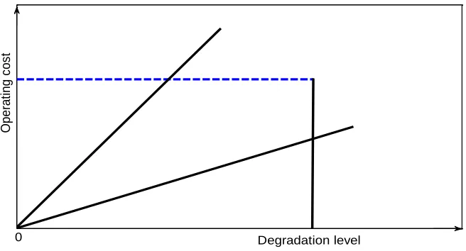
During system operation, the operating cost increases along with the degradation level, as shown in Fig 1. Generally, the age- and state-dependent operating cost can be modeled as a stochastic process, which depends on the degradation process. Decision-makers may have to take into account the two-dimensional degradation process when making maintenance policies. The operating cost may serve as a constraint on maintenance decision (for environmental issues) or an additional cost item (for economic concerns). However, little attention has been devoted to this important phenomenon in existing literature, which is further explained with the following two real-world examples.

Fig. 1 Plot of degradation level and operating cost evolvement

Modern vehicles are equipped with more and more sophisticated exhaust after-treatment facilities to satisfy increasingly stringent emissions limits. After a moderate mileage, vehicles may produce pollutant rates which largely exceed certification levels, despite of the on-board electronic control equipment. The increased pollutant rate is highly dependent on how the vehicle is used and maintained. With the traditional maintenance policy, an aged automobile is maintained only when

Degradation level

Opera

ting

c

os

t

it is failed (corrective maintenance) or is about to fail (preventive maintenance), while neither the side effect of increased energy consumption nor exhaust gas emission is considered.

Another example is the production system. In a production system, if a tool deteriorates over time, the quality of the produced products would decrease accordingly, which increases the rate of spoiled products (Xu & Cao, 2015). Traditional maintenance strategies focus on the tool itself, with little effort to the product quality as a result of tool aging and degradation. For a company,

retaining high quality and efficiency is essential in today’s heavy competition. A more appropriate

maintenance model is required to capture the operating cost due to aging and degradation. From the above two examples, one can see that there is a need to take the side effects along with aging and degradation into consideration when making maintenance decisions. This paper aims to satisfy this need. It regards the side effects due to aging and degradation as the operating cost and then develops a condition-based maintenance policy for degrading systems with consideration of the age- and state-dependent operating cost. The age- and state-dependent operating cost occurs when the system is operating in a deteriorated state, even if the system is still functioning. In studies with respect to integrated preventive maintenance and quality control models, some researchers have considered the age- and state-dependent operating cost (Tagaras, 1988; Yeung et al., 2008; Xiang, 2013). Yes there exist two substantial differences between our model and the previous models. The existing models considered the operating cost associated with the system itself, while our model can describe the side effect of degradation process on the other systems or environments. In addition, the previous models use discrete Markov chains to characterize the evolution of system state, while we employ a continuous stochastic process.

of the Wiener process, we model the CBM policy as a Markov decision process. The system is subject to periodic inspections. If the system has not failed at inspection, decision has to be selected among three maintenance actions: preventive replacement, repair and wait until the next inspection. The system is replaced when its degradation level exceeds a pre-specified threshold at inspection. The structural property of the optimal maintenance decision is investigated in depth and a monotone control limit policy is shown as the optimal strategy.

The novelty of this paper lies in the facts

 that the proposed maintenance model is able to capture the side effect due to system age

and degradation, and

 that decisions made based on this model not only consider the economic benefits, but also

the environmental and societal benefits.

We therefore claim that this is the first paper that incorporates side effect of degradation process into maintenance policies, which can be applied in various real systems to gain economic and societal benefits.

The remainder of this paper is organised as follows. Section 2 presents the degradation process and replacement model, where the maintenance cost function is derived and the structural properties of the optimal maintenance decision are further investigated. Section 3 formulates a more detailed maintenance decision with repair and replacement. Section 4 gives a numerical example to illustrate the maintenance decision and the associated managerial insights. Finally, Section 5 concludes the paper and suggests future research.

In this section, we develop an optimal replacement policy for a system subjected to the Wiener degradation process. The replacement model serves as the foundation for more sophisticated maintenance policies, e.g., the repair-replacement policy introduced in the next section.

2.1 Wiener degradation process

It is assumed that the system degrades according to the Wiener degradation process. The general form of the Wiener process is presented as

( ) ( ) ( ) ( )

dX t  t dt t dB t ₍₁₎

Taking integral of Eq (1), we have

X t( )M t( )  ( )t x0 ₍₂₎

where ( ) 0 ( ) t

M t 



and ( ) 0 ( ) ( ) t

t  s dB s

 



.

Usually, the initial degradation level at installation is 0, x0 0_{. Further, if the system is assumed} to go through a stationary Wiener process, which implies that  and  are constant, the degradation process is expressed as

0

( ) ( )

X t x  t B t

(3)

Note that the Wiener process is not monotonously increasing in time t, but its expectation E X t





is linearly increasing in t, i.e., E X t





identical independent increment properties (Guo et al, 2013; Ye & Xie, 2015). For any time sequence





normal distribution,













1 1 1

( )_i (_i ) _{i i} , _{i i}

X t X t_ N  t t_  t t_

The system is assumed to be failed when its degradation level hits a specific threshold l ,

( )

X t l_{. As the system state is fully revealed by the degradation level, we use the term “system}

state” and “degradation level” interchangeably in this paper.

2.2 Replacement model for system with operating cost

We consider the CBM policy in which periodic inspection is dedicated to monitor the degradation level of the system. We first consider the replacement model, where only preventive replacement is allowed to restore the system to a new state level. A sudden failure occurs when the degradation level exceeds the failure threshold l . Correspondingly, corrective replacement is carried out immediately to replace the failed system, with the corrective replacement cost cf _.

During the operation horizon, inspection is implemented periodically. At each inspection time, if the degradation level does not exceed the failure threshold, decision has to be made whether or not to preventively replace the system or let it be until the next inspection. The decision is made based on the current degradation level at inspection. If the system is replaced preventively, a preventive replacement cost cp _{is incurred. If one decides to wait until the next inspection, inspection cost} ci

is paid and the system runs the risk of sudden failure before the next inspection. It is assumed that both preventive maintenance and corrective maintenance restore the system to the as-good-as-new state. Apparently, cf cp _{, as} cf _{includes additional cost due to sudden failures, such as}

production loss and even life hazards.

likely to exhibit less efficiency and produce products with lower quality, taking a production line for example.

The system is inspected at equally spaced discrete time epochs,





each inspection, when the degradation level is detected, the sequence





the states of the sequential decision process. We follow the assumption of Elwany et al (2011): if the degradation level exceeds the failure threshold between inspections and then returns below the threshold at the next inspection, no failure is incurred.

The operating cost, G( ) , is dependent on both the system age and the system state. We assume that the operating cost is incurred only after the system age exceeds specific threshold, kc _{, where}

c

k

is a constant. Apparently the operating cost G t x( , ) exhibits the property that G t x( , ) is

non-decreasing in system age t and system state x . The degradation process of the system may influence the randomness of the operating cost in a complicated mechanism. Here, for simplicity, we assume the operating cost G t x( , ) as a linear function of the degradation level. G t x( , ) can be denoted as G t x t( , ( ))h t x t( ) ( ), where h t( )0, is a non-decreasing function of t. The assumption is reasonable in reality because the operating cost may increase rapidly for an aged or seriously degraded system.

Denote W k X





inspection to the (k+1)th inspection. Given the system age and state ( ,k Xk)_, W k X









, _k k ( , ( )) k ( ( )) ( , ( ))

k k

W k X E G t x t dt  f x t G t x t dxdt

 

  

 

 _{ }









where f x t( ( )) is the probability density function (pdf) of system state at time t.

Lemma 1. The expected operating cost within one period W k X





inspection epoch k and the observed system stateXk_.

The proofs of the lemmas and theorems in this paper are provided in Appendix.

The incurred cost has a discounting factor er during each inspection interval. Denote V k X( , k)

as the infinite-horizon minimal total discounted cost with the initial state( ,k Xk)_{. The optimality} decision satisfies the Bellman equation,













(0, 0)

( , ) min (0, 0) ,

, , ,

f k

k p

r r

k k k

c V X l

V k X c V

e U k X e W k X X l

  



_ 



 

 ₍₅₎

where U k X( , k)E V k





is the expected cost-to-go at the (k+1)th inspection.

Note that the inspection cost is treated as a separate cost item and not incorporated in Eq (5). The optimality equation follows the logic that (a) if the degradation level at the kth inspection exceeds the failure threshold l , which implies that the system is failed, then the system has to be replaced correctively; (b) if the system still functions, the decision maker can choose either to preventively replace the system or to let it be till the next inspection, depending on which is more cost-effective.

2.3 structural properties of the replacement policy

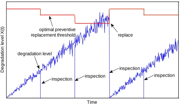
until the observed degradation level exceeds specific threshold (Benyamini & Yechiali, 1999). Fig. 2 shows the maintenance procedure and the evolvement of system state under control limit policy.

Fig. 2 Sketch of degradation process and maintenance actions Some essential properties are presented as follows.

Theorem 1. The value function, V k X( , k)_{, is non-decreasing in the inspection time k and system}

state Xk_.

Theorem 2. The optimal maintenance policy that minimises the value function, V k X( , k)_{, is a}

monotone control limit policy. At decision epoch k, preventive replacement is performed when the observed degradation level exceeds the optimal value k_{. The sequence}





The property of the monotone control limit policy can be incorporated into the optimisation algorithm to reduce the computational burden.

3. Replacement model with imperfect repair

Time

D

e

g

ra

d

a

ti

o

n

l

e

v

e

l

X

(t

)

inspection inspection

inspection

inspection replace

optimal preventive replacement threshold

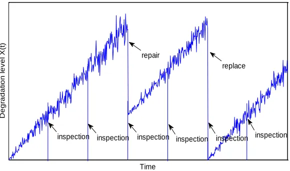
In this section, we consider the repair-replacement model, where repair is allowed to restore the system, in addition to replacement. Repair can be achieved by technical maintenance operations such as oiling and adding more lubricants (Zhang et al, 2015). It is assumed that the repair is imperfect, that repair restores the system to a state between as-good-as-new and as-bad-ad-old. At inspection, if the system still functions, three maintenance actions can be implemented: preventive replacement, repair, or wait until next inspection. Fig. 3 shows how the system state evolves under the repair-replacement strategy.

Fig. 3 Evolvement of system state under the repair-replacement model

3.1 Maintenance decision with controllable repair levels

At the decision epoch k with system state x, one can choose to repair the system to a lower level

( , )

y k x _{, where}y(0, ]x _{. y}x _{indicates that the system is left as it be.} 0 y x _{implies that the}

system is restored to a state between as-good-as-new and as-bad-as-old.

Denote the repair cost as C x y( , ). Of course it satisfies C x y( , )0, for yx. We assume that the repair cost C x y( , ) is increasing in x and decreasing in y, which implies that more resources have to be devoted to achieve more improvement of the system state (Özekici, 1995). If the system

Time

D

e

g

ra

d

a

ti

o

n

l

e

v

e

l

X

(t

)

repair

replace

inspection inspection

has failed at inspection, then corrective replacement is carried out. The corrective replacement cost

( , )

f

c C x y

, x y, 0. The difference between repair and replacement (either preventive or

corrective) is that repair can only restore the system state to a lower level, while replacement is able to restore both the system age and state to as-good-as-new condition. In addition, it is assumed that cp C x y( , )_, x y, 0_{. This assumption is reasonable because preventive replacement is}

more effective than repair and therefore incurs higher cost. Otherwise, repair makes no sense. Denote, again, V k X( , k) _{as the value function of the system starting with age k and state} Xk_. The Bellman equation is given as

























(0, 0)

min (0, 0) ,

( , )

inf ( , ) , , ,

, , ,

k

f k

p

r r

k

k y X

r r

k k k

c V X l

c V

V k X

C X y e U k y e W k y

e U k X e W k X X l

 

 

 



 

 

 

 

  _{ }

 

 

 ₍₆₎

Eq (6) implies that (a) if the system has failed at inspection, then corrective replacement is implemented; (b) if the system is operating, three maintenance actions can be selected: preventive replacement, repair to the optimal level, or wait until the next inspection, depending on which gives the minimal cost.

Lemma 2. The value function, V k X( , k)_{, is decreasing in the inspection epoch k and}

non-decreasing in Xk_.

Denote *

( )

k k

y X

as the optimal decision at the kth inspection with the observed state Xk_{, which} minimises the total expected discounted cost V k X( , k). More results can be obtained if restrictions

are imposed on the repair cost C x y( , ).

Theorem 3. Suppose C x y( , )C x z( , )C z y( , ), for all x z y. (1) If the optimal decision

at inspection is to repair the system, then

* * *

( ( )) ( )

y y x  y x _{for all x}_{0 . (2) If}

( , ) ( ) ( )

C x y c y c x _{, for} 0 y x_{, where} c( ) _{is a non-increasing cost, then} y x*( )

is non-decreasing in x.

Theorem 3 implies that if repair is the optimal decision, then it is more preferable to repair the system directly to state w, rather than repair the system to an intermediate state z ( x z w) then to state w. If the repair cost can be expressed as the difference of the current value and value after repair, the optimal repair level increases with the observed system state. This property can be used to reduce computational complexity of a search algorithm. The search interval of the optimal repair level

*

( )

k

y x

can be reduced by comparing the observed system state.

If the repair cost is only related to the repaired state y and independent of the current state x, we can conclude that the optimal maintenance policy between repair and doing nothing is a monotone control-limit policy.

Corollary 1. Suppose C x y( , )c y( ), for 0 y x, the optimal decision between repair and to do nothing is a control limit policy.

(1) At the kth inspection, there exists a critical value k_{, if the observed state}Xk k_{, then repair} should be carried out. Otherwise, the system should be left as it is.

(2) There exist a critical value * k

z

, the optimal repair level is

* *

( )

k k k

y X z

, for all lXk k_.

3.2 Maintenance decision with uncontrollable repair levels

In the previous analyses, the repair level is assumed to be controllable in the sense that the decision maker can determine to what level the system state can be restored to. However, in many cases, especially for complex systems, the repair level may be uncontrollable. Maintenance crew may try to repair the degraded system as much as possible; yet to which level the system state is restored depends on the degraded state before repair. The repair cost cre _{is assumed to be constant,}

independent of the system state. The system state after repair y x( ) satisfies the following properties: (1) 0 y x( )x; (2) y x'( )0, for all x(0, )l . The first property implies that the repair is imperfect. The second property indicates that the restored system state increases with the current state. In the literature, a great number of models have been established to describe the repair effect (Pham & Wang, 1996), among which, the virtual-age reduction model is widely used (Doyen & Gaudoin, 2004). Similar to the virtual-age reduction model, we establish a repair model where the system state after repair is proportional to the current state. Simply, we have

( ) (1 )

y x   x_{, where}  _{is a constant parameter, denoting the repair effect,} (0,1)_{. The}

optimal decision starting with the state ( ,k Xk) _{is given as}



 

 











(0, 0) min (0, 0) , ( , )

, , ,

, , ,

f k

p

k r r

re

r r

k k k

c V X l

c V V k X

c e U k y e W k y

e U k X e W k X X l

 

 

 

 

 

 

 

 

 



 _{ }

 ₍₇₎

Lemma 3. The optimal decision between repair and preventive replacement is a control-limit

Denote ( )

 

 

r r

k x e U k x e W k x

 

 _  _ 

, if k( )x _{is convex, it can be concluded that the}

optimal maintenance policy is of control-limit type.

Theorem 4. Suppose k( )x _{is a convex function, the optimal decision among preventive} replacement, repair or to do nothing is a control-limit policy. At the kth inspection, the optimal decision k _is

Preventive replacement, Repair,

Do nothing,

k k

k k k k

k k

if l X if X

if X

   



 

 

_  

 _



where k _and k _{are two critical values. In addition, the sequence}









are non-increasing in k.

Given the monotone property of the maintenance policy, the optimal policy can be obtained by many of the existing methods, e.g., value iteration algorithm and policy iteration algorithm (Puterman, 2014). Here, we adopt the monotone policy iteration to take advantage of the established structural properties. To make the solution feasible, we follow the existing practice to discretise the continuous state into finite intervals and use a time horizon long enough to approximate the infinite horizon. In particular, we define kmax _{as the maximum allowable system}

age for some integers kmax  _. kmax _{is set large enough so that the system will fail before} kmax

almost certainly. If the system survives beyond kmax _{, a preventive replacement is carried out to}

4. Numerical example

In this section, a diesel vehicle is presented to illustrate the maintenance policy. During service, the engine of the diesel vehicle is assumed to follow a Wiener degradation process with the drift coefficient 1 and diffusion coefficient  1. With the increase of usage and mileage, the engine may consume more diesels and produce more exhaust gas, which is modeled as the age- and state-dependent operating cost. Failures occur when the degradation level exceeds the failure threshold l6. The system is subject to periodic inspection, with the inspection interval  1 and the inspection cost ci 0.05 _{. At the kth inspection epoch, if the system functions but its} degradation level exceeds the control limit threshold, preventive replacement is carried out with cost cp 4_{. If the system has already failed, then corrective replacement is performed with cost}

10

f

c 

. The incurred cost is discounted with the discounting factor r 0.02. The total discounted

inspection cost is calculated separately as

0

exp( ) 2.52

1 exp( )

i

i i

k

c

U c rk

r









   

 



(8)

4.1 The age- and state-dependent operating cost

play a role (Pillot et al, 2014). Hence, we use a simple model to characterise the operating cost as a function of system age and degradation level. The operating cost of the system at age t and degradation level x is denoted as

( ) 0, ( , ) , c c t k c t k

G t x

e  x t k



  

 

  _

 ₍₉₎

where  and  are known parameters, scaling the effect of age and degradation level on the operating cost.

According to operating cost formulation, the cumulative operating cost between k _and k1 _is denoted as

1 1 ( )( )

( , ) k ( , ) k c ( )

k k

r t k k

Q k X  G t x dt  e  x t dt

  

  _{ }







, for k kc ₍₁₀₎

The expected operating cost within the interval ( , k k1)_{is given as}

















( , ) ( , ) k c ( )

k k c k t k k k t k

k k k

W k X E Q k X E e x t dt

E e X t B t dt

 _{ }   _{ }               _{  }      _     _  





, for k kc ₍₁₁₎

4.2 Optimal replacement policy and sensitivity analysis

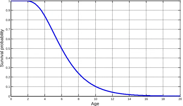
Fig. 4 Survival probability of degradation process

Fig. 5 plots the optimal maintenance policies with operating cost. It is clearly shown that the optimal maintenance policy is a monotone control limit policy, where the control limit shows a decreasing trend in system age. Whereas no operating cost is incorporated, as shown between age 0 and 4, the optimal maintenance policy is reduced to a constant control limit policy. This is due to the fact that the system degrades according to a homogeneous stochastic process and the system state increases independently after inspection. Compared with CBM policy where no age- and state-dependent operating cost is considered, the result shows a more conservative replacement threshold.

0 2 4 6 8 10 12 14 16 18 20

0 0.1 0.2 0.3 0.4 0.5 0.6 0.7 0.8 0.9 1

Age

S

u

rv

iv

a

l

p

ro

b

a

b

ili

Fig. 5 Optimal control limit policies with operating cost

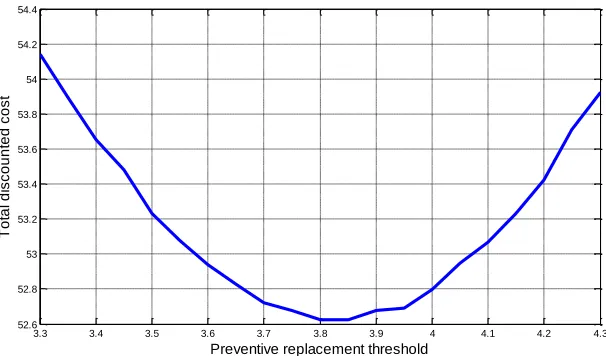
To investigate the effectiveness of the monotone control limit policy, we compare the monotone control limit policy with the traditional constant control limit policy. Fig. 6 shows how the total discounted cost varies under different preventive replacement thresholds. When the control limit is set as 3.85, the total discounted cost reaches its minimum 52.62. By comparison, the minimum total discount cost under monotone control limit policy is 48.45.

Fig. 6 Cost variation of constant control limit policy

0 1 2 3 4 5 6 7 8 9 10

2.5 3 3.5 4 4.5

Age

C

o

n

tr

o

l

lim

it

k

Constant control limit

Replace

Not replace

3.3 3.4 3.5 3.6 3.7 3.8 3.9 4 4.1 4.2 4.3

52.6 52.8 53 53.2 53.4 53.6 53.8 54 54.2 54.4

Preventive replacement threshold

T

o

ta

l

d

is

c

o

u

n

te

d

c

o

s

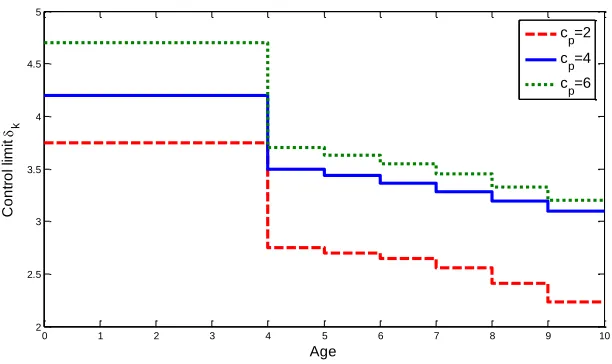
We are interested in finding how the optimal control limit policy changes against various cost parameters. Sensitivity analysis is therefore conducted to investigate this relationship, as presented in Fig. 7 and Fig. 8. When the preventive replacement cost cp _{becomes closer to the corrective}

replacement cost cf _{, the optimal control limit policy is more tolerant to system failure. In other}

words, the optimal maintenance policy is less conservative. As shown in Fig. 7, with the increase of preventive replacement cost, the optimal control limit k _{shows an increasing trend. The result} is quite straightforward. It is less attractive to preventively replace the system when the preventive replacement cost increases. On the other hand, an increased corrective replacement cost cf _results

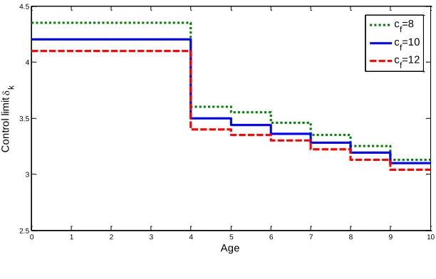
in a more conservative control limit policy, as shown in Fig. 8. As can be observed from Fig. 7 and Fig. 8, the influence of different cf _{is not so significant as that of} cp_{. This can be explained}

as that the optimal control limits are far from the failure threshold and sudden failure occurs infrequently. Therefore, the corrective replacement cost cf _{has less influence on the optimal}

control limits.

Fig. 7 Sensitivity analysis for cp

0 1 2 3 4 5 6 7 8 9 10

2 2.5 3 3.5 4 4.5 5

Age

C

o

n

tr

o

l

lim

it

k

c

p=2

c

p=4

c

Fig. 8 Sensitivity analysis for cf

5. Conclusion

This paper develops a condition-based maintenance policy for systems with age- and state-dependent operating cost. The system is subject to a continuous degradation process, characterised by a Wiener process with linear drift. The operating cost occurs during system operation, which increases with system age and the degradation level. Two models capable of arriving at maintenance decisions are developed. One is the replacement model and the other is the repair-replacement model. The structural properties of the optimal decision are investigated in depth. For the replacement model, this paper show that the optimal decision is actually a monotone control limit policy. For the repair-replacement model, it shows that, under mild assumptions of the repair cost, the optimal decision among preventive replacement, repair and doing nothing is also a monotone control limit policy. A numerical example is presented to illustrate the optimal maintenance decisions.

The proposed model can be applied in various systems. For example, in a power grid, the resistance of electric wire increases with the age and degradation level of power line, which

0 1 2 3 4 5 6 7 8 9 10

2.5 3 3.5 4 4.5

Age

C

o

n

tr

o

l

lim

it

k

c

f=8

c

f=10

consumes more energy when transmitting electricity. The energy loss due to age and degradation can be modeled as the age- and state- dependent operating cost, and the proposed maintenance model can be used to capture the energy loss during power transmission.

Future extensions of this study can be conducted with respect to a non-stationary degradation process. The Wiener process with linear drift is only available to a limited number of systems, which fails to describe a complicated degradation process. Extension to a more general class of degradation process will remedy this disadvantage. Additionally, in the current work, we assume that inspection can fully reveal the underlying degradation level, which may be relaxed by considering imperfect inspection. In the imperfect inspection framework, the maintenance decision can be formulated as a partially observable Markov decision process.

Acknowledgement

The work was completed while the first author was visiting Shaomin at University of Kent and we appreciate the support from City University of Hong Kong and University of Kent that made this possible.The work described in this paper was partially supported by a theme-based project grant (T32-101/15-R) of University Grants Council, and a Key Project (71532008) supported by National Natural Science Foundation of China.

Appendix

1. Proof of Lemma 1.





0

( 1) ( 1)

, ( ( )) ( , ( )) ( ( )) ( ) ( ) ( ) ( ) k k _k k k k k

k _{k k}

W k X f x t G t x t dxdt f x t h t x t dxdt

X h t dt th t dt

                  













Define ( ) 0 ( ) t

H t 



, so that H t'( )h t( )0 and H t''( )h t'( )0. As h t( )0, it can be

easily observed that W k X









k, we only need to prove that ( 1)

( )

k

k h t dt



 



( )

k

k th t dt



 



Let

( 1)

( ) k ( )

k

k h t dt

 

 

_

and

( 1)

( ) k ( )

k

k th t dt

 

 

_

. We have





 





( ) ( 1) ( )

( 2) 2 ( 1)

k k k

H k  H k H k 

     

    

AsH t'( )h t( )0 and H t''( )h t'( )0, H t( )is a convex function in t. The Jensen’s inequality (Boyd & Vandenberghe, 2004) states that





1 2 1 2

( ) (1 ) ( ) (1 )

f x f x f x x

      

for any convex function f( ) and (0,1). With the above inequality, we can readily obtain that





 





( )k H (k 2) H k 2H (k 1) 0

      

(A2)

Let q t( ) t h t( ). Clearly q t( ) is increasing in t and 0 ( ) t

q u du



we can have

( )k (k 1) ( )k 0

       _(A3)

Combining Eq. (A2) and Eq. (A3), we have W k X





2. Proof of Theorem 1.

Proof. We prove the theorem by mathematical induction. Denote ( , ) n

k

V k X

as the value

function at the nth iteration of value iteration policy. At n0, we set 0

( , _k) V k X

=0, which is a

constant. Assume that the theorem holds for the nth iteration, i.e., ( , ) n

k

V k X

is non-decreasing in

k and non-decreasing in Xk_{. Then according to Eq (5), we have}













1

(0, 0)

( , ) min (0, 0) ,

, , ,

n

f k

n n

k p

r n r

k k k

c V X l

V k X c V

e U k X e W k X X l

       _     

Lemma 1 shows that W k X





k

V k X

is non-decreasing

in k and non-decreasing in Xk_{, its expectation,}





k U k X

, holds this property as well. Because

the terms of the right-hand side are non-decreasing in k and non-decreasing in Xk_, 1

( , )

n

k

V  k X

is

also non-decreasing in k and Xk_{, which completes the proof.}

3. Proof of Theorem 2.

Proof. Preventive maintenance is optimal when (0,0)









r r

p k k

c V eU k X eW k X

. The

left-side is a constant. Based on Theorem 1,









r r

k k

eU k X eW k X

is non-decreasing in Xk_.

Thus for any Xk k_{, the inequality holds, which implies the monotone control limit policy. On}

the other hand, the term on the right-hand side is non-decreasing in k. Therefore, for the inspection epoch k, there exists an optimal replacement age k , such that for any kk, the optimal decision

4. Proof of Theorem 3.

Proof. (1) As repair is the optimal decision at the kth inspection, we have









* * *

( , ) ( , ) r , r ,

V k x C x y eU k y eW k y

. If *

( )

y x x

, then obviously.

If *

( )

y x  z x

, we need to prove that *

( )

y z z

. Suppose not, then *

( )

y z  w z

. Then we have

 

 

( , ) ( , ) r , r ,

V k x C x z eU k z eW k z

< ( , )









r r

C x w e U k w e W k w

(B1)

This inequality holds because *

( )

y x z

is the optimal repair level, which restores the system

to state w and incurs more cost. In addition, we have









 

 

 

 

( , ) ( , ) , , ( , )

( , ) , , , ,

r r

r r r r

V k w C z w e U k w e W k w V k z

C z z e U k z e W k z e U k z e W k z

                     (B2)

This inequality holds because repairing the system to state *

( )

y z w

is more cost-effective than

to do nothing until the next inspection, according to the assumption . Combining Eq (B1) and Eq (B2), we have

 

 









( , ) r , r , r , r , ( , ) ( , )

C z w e U k z e W k z e U k w e W k w C x w C x z

(B3)

so that we have C z w( , )C x z( , )C x w( , ) , which is contradictory to the assumption

. Hence, it can be concluded that , and .

(2) To prove this result, we need to show that

* *

( ) ( )

y x u  y x

, for any u0. Consider the case that repair is the optimal decision at inspection. We can have





































( , ) inf ( ) ( ) , ,

inf ( ) ( ) , , ,

min

inf ( ) ( ) , ,

r r

y x u

r r

y x

r r

x y x u

V k x u c y c x u e U k y e W k y c y c x u e U k y e W k y

c y c x u e U k y e W k y

                                 _{ }         If * ( )

y x u x

, then

* * *

( ( )) ( )

y y x y x

*

( )

y z  w z

( , ) ( , ) ( , )













( , ) inf ( ) r , r , ( )

y x

V k x u c y e U k y e W k y c x u



     

In addition, we have













( , ) inf ( ) r , r , ( )

y x

V k x c y e U k y e W k y c x



   

Combine the above two expressions, it can be readily obtained that

* *

( ) ( )

y x u  y x

, for *

( )

y x u x

.

If *

( )

x y x u  x u _{, then obviously,} y x u*(  )y x*( )_{, as} y x u*(  ) x y x*( )_{. Therefore,}

*

( ) y x

is non-decreasing in x, for all 0 y x.

5. Proof of Corollary 1.

Proof. (1) If preventive replacement is not a preferable option, we can have

 

 

















min inf ( ) , , ,

( , ) , , k r r y X k r r k k

c y e U k y e W k y V k X

e U k X e W k X

          _{ }     _

 _(C1)













inf ( ) , ,

k

r r

y X c y e U k y e W k y

 

 

   _{is non-increasing in} Xk _{because the interval} (0,Xk)

becomes wider, which relaxes the constraints of y. On the other hand,









r r

k k

e U k X e W k X

is increasing in Xk_{, as shown in Theorem 1. Thus, the minimum of}

the two functions has to satisfy

 

 















inf ( ) , , ,

( , ) , , , k r r k k y X k r r

k k k k

c y e U k y e W k y if X V k X

e U k X e W k X if X

            _{  }     

 _(C2)

where

























inf 0 : inf ( ) , , , ,

k

r r r r

k k k k

y X

X c y e U k y e W k y e U k X e W k X

    



     

(2) If Xk k_{, we can easily have} * k k

y X

, implying that no repair is carried out if Xk k_.

On the other hand, if Xk k_{, then} ( , ) infk













r r

k y X

V k X c y e U k y e W k y



  

according

to Eq (C2). Because infk













r r

y X c y e U k y e W k y

 

 

   _{is decreasing in} Xk[k, ) _while

( , _k) V k X

is increasing in Xk_{, the only way they are equal is that} V k X( , k)_{is a constant;} V k X( , k)

=V k( ,k) _{for all} Xk[k, ) _{. Therefore, we can conclude if}

* *

( _k) _k

y  z

, then

* *

( )

k k k

y X z

, for

all Xk[k, ) _.

(3) The proof is analogous to Theorem 2. The details are not shown here to avoid repetition.

6. Proof of Lemma 3

Proof. According to the assumption, the restored system state y increases with the current state k

X

. Meanwhile, both U k y

 

 

concluded that U k y X









(0, 0)

p

c V

is independent of Xk _{. Thus, there exists a critical value} k _{, such that}

 

 

( _k) r , r , _p (0, 0) C X e U k y e W k y c V

, forXk k_.

7. Proof of Theorem 4.

Proof. Lemma 3 shows that preventive replacement is preferred over repair for Xk k_{. Next,}

we need to prove that repair is preferred over doing nothing for k  Xk k _{. Let}





( ) ( ) ( )

k x cre k y x k x

   

. We have ' ( )k x ' ( ) '( )k y y x ' ( )k x _{. According to the}

y x _{, we can have} ' ( )k x 0 _{, which implies that} k( )x _{decreases in x . Because}

(0) 0

k cre

   _{, and}k( )x 0_{, for x} _{. Hence, we can conclude that there exists a critical}

value k_{, repair is preferred over doing nothing for} k Xk k_{. As all the right-hand items of}

Eq (8) increase with k, we can conclude that the sequence









Reference

Benyamini, Z., & Yechiali, U. (1999). Optimality of control limit maintenance policies under nonstationary deterioration. Probability in the Engineering and Informational Sciences, 13(01), 55-70.

Boyd, S., & Vandenberghe, L. (2004). Convex optimization. Cambridge university press.

Chen, N., Ye, Z. S., Xiang, Y., & Zhang, L. (2015). Condition-based maintenance using the inverse Gaussian degradation model. European Journal of Operational Research, 243(1), 190-199. Doyen, L., & Gaudoin, O. (2004). Classes of imperfect repair models based on reduction of failure

intensity or virtual age. Reliability Engineering & System Safety, 84(1), 45-56.

Elwany, A. H., Gebraeel, N. Z., & Maillart, L. M. (2011). Structured replacement policies for components with complex degradation processes and dedicated sensors. Operations Research, 59(3), 684-695.

Guo, C., Wang, W., Guo, B., & Si, X. (2013). A maintenance optimization model for mission-oriented systems based on Wiener degradation. Reliability Engineering & System Safety, 111, 183-194.

Hsu, B. M., & Shu, M. H. (2010). Reliability assessment and replacement for machine tools under wear deterioration. The International Journal of Advanced Manufacturing Technology, 48(1-4), 355-365.

Jardine, A. K., Lin, D., & Banjevic, D. (2006). A review on machinery diagnostics and prognostics implementing condition-based maintenance. Mechanical Systems and Signal Processing, 20(7), 1483-1510.

Jeang, A. (1998). Reliable tool replacement policy for quality and cost. European Journal of Operational Research, 108(2), 334-344.

Lam, J. Y. J., & Banjevic, D. (2015). A myopic policy for optimal inspection scheduling for condition based maintenance. Reliability Engineering & System Safety, 144, 1-11.

Liu, B., Xie, M., & Kuo, W. (2016). Reliability modeling and preventive maintenance of load-sharing systems with degrading components. IIE Transactions, 48(8), 699-709.

Liu, B., Xu, Z., Xie, M., & Kuo, W. (2014). A value-based preventive maintenance policy for multi-component system with continuously degrading components. Reliability Engineering & System Safety, 132, 83-89.

Özekici, S. (1995). Optimal maintenance policies in random environments. European Journal of Operational Research, 82(2), 283-294.

Pham, H., & Wang, H. (1996). Imperfect maintenance. European Journal of Operational Research, 94(3), 425-438.

Pillot, D., Legrand-Tiger, A., Thirapounho, E., Tassel, P., & Perret, P. (2014, April). Impacts of inadequate engine maintenance on diesel exhaust emissions. In Transport Research Arena (TRA) 5th Conference: Transport Solutions from Research to Deployment.

Puterman, M. L. (2014). Markov decision processes: discrete stochastic dynamic programming. John Wiley & Sons.

Si, X. S., Wang, W., Hu, C. H., Chen, M. Y., & Zhou, D. H. (2013). A Wiener-process-based degradation model with a recursive filter algorithm for remaining useful life estimation. Mechanical Systems and Signal Processing, 35(1), 219-237.

Tagaras, G. (1988). An integrated cost model for the joint optimization of process control and maintenance. Journal of the Operational Research Society, 39(8), 757-766.

Whitmore, G. A., & Schenkelberg, F. (1997). Modelling accelerated degradation data using Wiener diffusion with a time scale transformation. Lifetime Data Analysis, 3(1), 27-45. Wu, X., & Ryan, S. M. (2010). Value of condition monitoring for optimal replacement in the

proportional hazards model with continuous degradation. IIE Transactions, 42(8), 553-563. Xiang, Y. (2013). Joint optimization of control chart and preventive maintenance policies: A

discrete-time Markov chain approach. European Journal of Operational Research, 229(2), 382-390.

Xu, W., & Cao, L. (2015). Optimal tool replacement with product quality deterioration and random tool failure. International Journal of Production Research, 53(6), 1736-1745.

Ye, Z. S., Shen, Y., & Xie, M. (2012). Degradation-based burn-in with preventive maintenance. European Journal of Operational Research, 221(2), 360-367.

Ye, Z. S., & Xie, M. (2015). Stochastic modelling and analysis of degradation for highly reliable products. Applied Stochastic Models in Business and Industry, 31(1), 16-32.

Yeung, T. G., Cassady, C. R., & Schneider, K. (2007). Simultaneous optimization of [Xbar] control chart and age-based preventive maintenance policies under an economic objective. IIE transactions, 40(2), 147-159.