Automatic Exposure Control,
Radiometric Calibration and
Dynamic Range Compression
Ahmed Sohaib
A thesis submitted for the degree of
Doctor of Philosophy at
I would like thank Almighty Allah for guiding me, and giving me strength to achieve this milestone. I am grateful to my primary supervisor, Dr. Antonio Robles-Kelly, for his energies, efforts, and guidance. I have always found him encouraging and motivating to work. His positive energy has driven my work to this end. I would also like to thank my co-supervisor, Dr. Nariman Habili, for his time to review my drafts and his concerned advices whenever needed. I would like to thank Dr. Hongdong Li for taking up the role of adviser and being part of my supervisory panel. His research contributions are inspiration to many.
I would like to thank The Australian National University and National ICT Aus-tralia for funding my PhD and providing a great learning and research environ-ment. I am grateful to the staff and students of Canberra Research Lab at NICTA for their support and fellowship. I am also grateful to our Imaging Spectroscopy and Scene Analysis (ISSA) research team (Ran Wei, Cong Huynh, Lin Gu, Sejuti Rahman, Lawrence Mutimbu, Luis Romero-Ortega, and Arash Shahriari) for their wonderful support and discussions that paved my research path. I must thanks Khurrum Aftab, Adnan Shah, Saeed Anwar, Muhammad Hanif, Muhammad Usman, Zeeshan Hyder, Behrooz Nasihatkoon, and many others for their acquaintance and making my stay in Australia comfortable and enjoyable. I must thank the wonderful Canberra Com-munity for making my stay in Canberra memorable and cherishing. It was a great learning experience living in a multi cultural place like Canberra.
In the end, I would like to thank my father, who passed away during my PhD, for his sacrifices and devotion to see my achievements. I would also like to thank my mother for her prayers and sacrifices for my success in every step of my life. I am also thankful to my sisters for their encouragement and prayers. Finally, I owe a lot to my wife, my son, and my daughter for bearing with me the difficulties of studentship abroad, and always there to comfort me with their joyful company.
Imaging systems are essential to a wide range of modern day applications. With the continuous advancement in imaging systems, there is an on-going need to adapt and improve the imaging pipeline running inside the imaging systems.
In this thesis, methods are presented to improve the imaging pipeline of digi-tal cameras. Here we present three methods to improve important phases of the imaging process, which are (i) “Automatic exposure adjustment” (ii) “Radiometric calibration” (iii) ”High dynamic range compression”. These contributions touch the initial, intermediate and final stages of imaging pipeline of digital cameras.
For exposure control, we propose two methods. The first makes use of CCD-based equations to formulate the exposure control problem. To estimate the exposure time, an initial image was acquired for each wavelength channel to which contrast adjustment techniques were applied. This helps to recover a reference cumulative distribution function of image brightness at each channel. The second method pro-posed for automatic exposure control is an iterative method applicable for a broad range of imaging systems. It uses spectral sensitivity functions such as the pho-topic response functions for the generation of a spectral power image of the captured scene. A target image is then generated using the spectral power image by applying histogram equalization. The exposure time is hence calculated iteratively by mini-mizing the squared difference between target and the current spectral power image. Here we further analyze the method by performing its stability and controllability analysis using a state space representation used in control theory. The applicability of the proposed method for exposure time calculation was shown on real world scenes using cameras with varying architectures. Radiometric calibration is the estimate of the non-linear mapping of the input radiance map to the output brightness values. The radiometric mapping is represented by the camera response function with which the radiance map of the scene is estimated. Our radiometric calibration method em-ploys an L1 cost function by taking advantage of Weisfeld optimization scheme. The
proposed calibration works with multiple input images of the scene with varying ex-posure. It can also perform calibration using a single input with few constraints. The proposed method outperforms, quantitatively and qualitatively, various alternative methods found in the literature of radiometric calibration.
Acknowledgments vii
Abstract ix
1 Introduction 1
1.1 Overview . . . 4
1.2 Contributions . . . 5
1.2.1 Automatic Exposure Control for Spectral Cameras Using His-togram Equalization . . . 5
1.2.2 Automatic Exposure Control For Cameras Using Optimization . 6 1.2.3 Radiometric Calibration of Cameras . . . 6
1.2.4 Compressing Dynamic Range of Images for display . . . 7
2 Background and Related Work 9 2.1 Related terminologies . . . 9
2.2 Background . . . 10
2.3 Related work . . . 13
2.3.1 Exposure Control for Cameras . . . 13
2.3.2 Radiometric Calibration . . . 15
2.3.3 High Dynamic Range Compression . . . 18
3 Automatic Exposure Control for Spectral Cameras Using Histogram Equal-ization 21 3.1 CCD representation for spectral camera . . . 23
3.2 Exposure Time Recovery Using Histogram Equalization Technique . . . 25
3.3 Experiments . . . 27
3.4 Summary . . . 32
4 Controllable Automatic Exposure Adjustment for Cameras 35
4.1 Method . . . 36
4.2 Stability Analysis . . . 41
4.2.1 State Space Representation . . . 41
4.2.2 Stability Analysis of the method . . . 43
4.2.3 Controllability . . . 44
4.3 Results and Discussion . . . 46
4.4 Summary . . . 54
5 Radiometric calibration 57 5.1 Estimating the Camera Response and Radiance Map . . . 59
5.2 Initialization . . . 61
5.3 Single Image Radiometric Calibration . . . 62
5.4 Experiments . . . 65
5.4.1 Results for Multiple Image Radiometric Calibration . . . 65
5.4.2 Results for Single Image Radiometric Calibration . . . 77
5.4.3 Results on Panorama Images . . . 78
5.5 Time Complexity of the algorithm . . . 79
5.6 Summary . . . 79
6 High dynamic range compression 83 6.1 Method . . . 84
6.2 Exposure Selection . . . 87
6.3 Experiments . . . 88
6.4 Summary . . . 98
7 Conclusion 101 7.1 Summary . . . 101
7.2 Future Work . . . 103
1.1 Abstract level Image acquisition pipeline of digital cameras proposed by (Debevec and Malik [1997]) . . . 2
1.2 Our first contribution in proposing automatic exposure adjustment for cameras . . . 2
1.3 Our second contribution in proposing radiometric calibration of cam-eras . . . 3
1.4 Our third contribution in proposing dynamic range compression of radiance map images for out images to digital displays . . . 5
2.1 Abstract level Image acquisition pipeline of digital cameras proposed by Debevec and Malik [1997] . . . 10
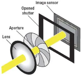
2.2 Graphical representation of light reaching imaging sensor through lens, aperture, with a desired shutter speed. . . 11
3.1 Effect of exposure time changes on the image brightness. From left-to-right: Pseudo-colour images (hyperspectral images from Foster dataset (Foster et al. [2006]), rendered into colour using the CIE colour match-ing function in CIE [1932]) acquired with increasmatch-ing exposure times. Note the image detail is lost at either extreme of the timings, whereby the imagery is underexposed or saturated. . . 22
3.2 Sample wavelength indexed-bands for a hyperspectral image depicting a landscape. From left-to-right: Bands corresponding to 480nm, 520nm and 680nm. . . 23
3.3 From left-to-right: Pseudo color image acquired using random expo-sure times set, equalisation results for both, the uniform and Gaussian distributions and imagery acquired using the exposure times yielded by our method for the two equalisation targets. . . 28
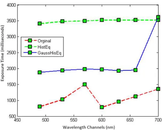
3.4 Exposure times as a function of wavelength index for the imagery in Figure 3.3. X-axis represents the wavelength channels in nm. Y axis represents the exposure time in milliseconds. . . 29
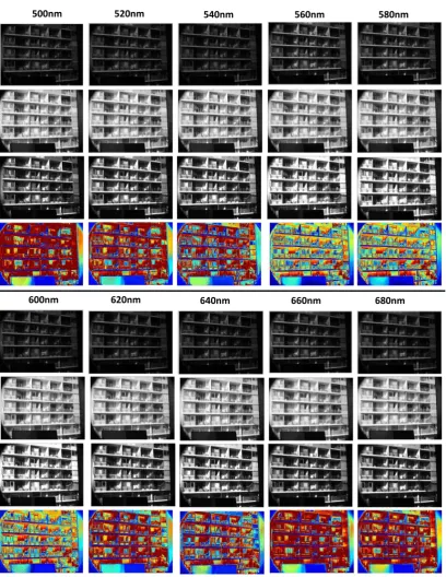
3.5 Results yielded by our method per wavelength indexed band. For both top and bottom panels, each column, from top-to-bottom shows: Band acquired using a randomly selected exposure time, histogram equalised image, wavelength-indexed band acquired using the expo-sure time yielded by our method and per-pixel normalised error map. For the error maps, red represents a value of 1 and blue amounts to zero. 30
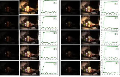
3.6 Results of our method for 10 trials corresponding to randomly selected exposure times as input to our method. For each of the two pan-els in the figure, each row corresponds to, from left-to-right, pseudo colour image for the images acquired using randomly selected expo-sure times, imagery captured using the times delivered by our method, time plots showing the initial and recovered exposure times as a func-tion of wavelength index. . . 31
3.7 Mean exposure times for the 10 trials in Figure 3.6. X axis represents the wavelengths and Y axis represents the exposure time. . . 32
4.1 Photopic response function depicting spectral sensitivity of human vi-sual system when exposed to brightness . . . 37
4.2 FluxData multi-spectral camera scenes. Left-hand column: Spectral power image; Right-hand column: Color chart gray-tile intensity plots (the x-axis corresponds to the index of the tile and the y-axis to the photopic response). In the figure, the top row shows the initial im-ages, whereas the second row corresponds to the images produced by the exposure times at the iteration corresponding to the middle point over the convergence of our method. The third row shows the image acquired using the exposure time yielded by our method after conver-gence has been reached. Finally, the bottom row shows the normalised error plots as a function of iteration number. . . 48 4.3 OKSI hyperspectral camera scenes. Left-hand column: Spectral power
image; Right-hand column: Color chart gray-tile intensities (thex-axis corresponds to the index of the tile and they-axis to the photopic re-sponse). In the figure, the top row shows the initial images, whereas the second row corresponds to the images produced by the exposure times at the iteration corresponding to the middle point over the con-vergence of our method. The third row shows the image acquired using the exposure time yielded by our method after convergence has been reached. Finally, the bottom row shows the normalised error plots as a function of iteration number. . . 50
4.5 Spectral power images for the color chart using the exposure times obtained manually (left) and those obtained using our method (right). . 52
4.6 Photopic response as a function of the indices of the gray-scale tiles in the Macbeth ColorChecker for our method (solid line) and the manu-ally exposed image (broken line). . . 53
4.7 RGB images for indoor and outdoor scenes acquired by first placing color chart to determine exposure time with help of grayscale tiles (Shown in left-most column). Baseline images were acquired using manually computed exposure times shown in middle column. In the right-most column results shown are yielded by our method . . . 55
5.1 Spectral sensitivity of the Nikkon D80 (left) used on the Foster dataset; Cannon 20D spectral sensitivity (right) used for the Scyllarus datasets. . 66
5.2 Camera response functions used to render our LDR imagery. Top row: Optura 981-114 CCD; Bottom row: Sony DX-9000- CCD. From left-to-right: Red, green, and blue channels. . . 67
5.3 Radiance and LDR images for a sample scene used in our experiments. From left-to-right: Ground truth normalised radiance image and LDR images generated using exposure time of 1/250, 1/125, 1/60 , 1/30 and 1/15 seconds, respectively. . . 67
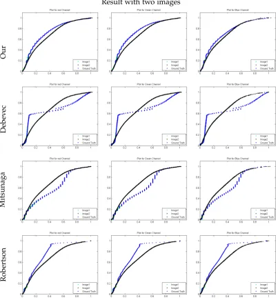
5.5 Camera response functions calculated using two images for a sample scene on the Foster dataset shown in Figure 5.3. From top-to-bottom: Resulsts delivered by our’s, Debevec’s , Mitsunaga’s and Robertson’s methods. The plots from left to right represent the red, green , and blue channels. The black curve in all the plots accounts for the ground truth camera response used to render the imagery. . . 70
5.6 Radiance images , tonemapped radiance image and the error image generated by methods using three images for the sample scene on the Foster dataset shown in Figure 5.3. From top-to-bottom: Results de-livered by our’s, Debevec’s , Mitsunaga’s and Robertson’s methods. The error images are generated using the ground truth and methods generated image. Error images are normalized where red represents 1 and blue represents 0 . . . 71
5.7 Camera response functions calculated using three images (1/250s, 1/60s and 1/15s) for a sample scene on the Foster dataset shown in Figure 5.3. From top-to-bottom: Resulsts delivered by our’s, Debevec’s , Mit-sunaga’s and Robertson’s methods. The plots from left to right rep-resent the red, green , and blue channels. The black curve in all the plots accounts for the ground truth camera response used to render the imagery. . . 72
5.9 Camera response functions calculated using five images for a sample scene on the Foster dataset shown in Figure 5.3. From top-to-bottom: Results delivered by our’s, Debevec’s , Mitsunaga’s and Robertson’s methods. The plots from left to right represent the red, green , and blue channels. The black curve in all the plots accounts for the ground truth camera response used to render the imagery. . . 74 5.10 Left-hand column: Camera response function for the Optura 981114
CCD recovered by our method and the alternatives when two LDR images are used; Right-hand column: Camera response function re-covered when three LDR images are used at input. The rows, from top-to-bottom show the functions for each of the colour channels, i.e. red, green and blue. . . 76 5.11 Left to right: Input LDR image for SIRC, Groundtruth camera response
curve, Groundtruth irradiance image taken from CRF and input LDR image . . . 77 5.12 Irradiance image and camera response function for the Optura 981114
CCD recovered by our method when using single LDR image. Top to bottom: First row shows the irradiance image and CRF of red, green and blue channel at first iteration. Second row shows the irradiance image and CRF at the middle of iteration. Bottom row shows the result at final iteration. . . 78 5.13 Panoramas generated by stitching HDR tone-mapped images
deliv-ered by ours, Debevec’s , Mitsunaga and Robertson’s method. . . 80
5.14 Panoramas generated by stitching tone-mapped HDR views using 2 LDR images. (From left to right) Results yielded by our’s (1st col-umn) Debevec’s (2nd colcol-umn); Mitsunaga’s (3rd colcol-umn) and Robert-son’s (4th column) methods.First row shows the generated results ; second and third row shows the cropped regions magnified for re-spective method . . . 81 5.15 Panoramas generated by stitching HDR tone-mapped images
6.1 LDR images at different exposure obtained using exposure selection approach for two scenes: top panel first scene; bottom panel second scene . . . 89
6.2 Contrast Images and probability images generated by our method us-ing LDR images obtained by exposure selection. For both left and right panel the first column contains the LDR images generated by the ex-posure selection, second column contains the contrast images obtained from the LDR images and the third column represents the probability images generated from the corresponding contrast images. Last row shows the resultant compressed dynamic range image, and its gamma corrected image. Gamma used for correction is 2.2 . . . 90
6.3 Contrast Images and probability images generated by our method us-ing LDR images obtained by exposure selection. For both left and right panel the first column contains the LDR images generated by the ex-posure selection, second column contains the contrast images obtained from the LDR images and the third column represents the probability images generated from the corresponding contrast images. Last row shows the resultant compressed dynamic range image, and its gamma corrected image. Gamma used for correction is 2.2 . . . 91
6.4 High dynamic range images widely used for method comparisons. We use these HDR images to test the dynamic range compression tech-nique proposed in this paper in comparison with results of methods used professionally and cited in literature. . . 92
6.6 Comparison of our method results with the results of methods widely available and cited in literature. For each method the first column contains the gamma corrected output and second column contains the output of the dynamic range independent image quality assessment (DRIMQA) for the respective method . . . 95 6.7 Comparison of our method results with the results of methods widely
available and cited in literature. For each method the first column contains the gamma corrected output and second column contains the output of the dynamic range independent image quality assessment (DRIMQA) for the respective method . . . 96 6.8 Comparison of our method results with the results of methods widely
available and cited in literature. For each method the first column contains the gamma corrected output and second column contains the output of the dynamic range independent image quality assessment (DRIMQA) for the respective method . . . 97
4.1 Equivalence between the variables in the state space equations and those used in Section 4.1. Here we haver =| I |+ |e[k]|;s =| Iˆ|+c
; and q= c, where | . |yields the number of elements in the array or vector under consideration. . . 43
5.1 RMS error and standard deviation across each of the datasets under study for ours, Debevec’s, Mitsunaga’s, and Robertson’s methods. . . . 75
6.1 Table showing Loss of contrast of method for different images . . . 94 6.2 Table showing amplification of contrast of method for different images 98 6.3 Table showing reverse of contrast of method for different images . . . . 99
Introduction
Imaging systems are central to modern day life. Ranging from space exploration (Martin et al. [2005]) to microscopic level studies (Lang et al. [2002]) imaging sys-tems have a vital role to play. Imaging syssys-tems are also widely used today in hand held devices (Rohs and Gfeller [2004]) as well as in entertainment (Zhang [2012]) and mass media (Kubota et al. [1996]). Medical imaging has recently evolved as an important domain for non invasive diagnosis and life sciences studies (Groezinger [2000]). Remote sensing is a domain where spectral imagers are used for mining (Riley and Hecker [2013]), agriculture (Thenkabail et al. [2016]), surveillance (Pajares [2015]) and environmental (Nagendra et al. [2013]) applications. Spectral imagers are an important tool for material studies in material sciences (McCrindle et al. [2014]). Imaging systems are used in system automation (Yang et al. [2014]) and in the do-main of robotics (Nagatani et al. [2013]) to perform extreme tasks. They also play an important role in quality assurance in food (Wu and Sun [2013]) and industry (Nevalainen and Pellinen [2016]). With the evolution of new technologies, there is a rise of a wide spectrum of applications which demand update and upgrade in imaging systems under use. Thus there is a continuous need to improve the imag-ing systems pipeline. In this thesis methods have been proposed to improve the imaging pipeline for a broad range of imaging systems including traditional RGB cameras as well as modern day multispectral and hyperspectral cameras. These in-clude exposure control, radiometric calibration and dynamic range compression for low dynamic range display devices. To better understand the thesis contribution to-wards improving the imaging pipeline, we show, in Figure 1.1, an abstraction of the image acquisition pipeline presented by (Debevec and Malik [1997]).
Figure 1.1: Abstract level Image acquisition pipeline of digital cameras proposed by (Debevec and Malik [1997])
At the abstract level, part of scene radiance passes through the lens, the aper-ture, and some desired filters to reach the sensor. At this stage, the imaging sensor (charged couple device CCD in this case) is exposed to the incoming light for a given exposure time (shutter speed) to generate photoelectrons. These photoelectrons are then converted to digital values using an analog to digital converter. After that, few on-board operations (e.g. noise reduction, sharpening, demosaicing, white balance, tone-mapping) are performed on the digital values. Finally, pixel values are obtained that are nonlinear with respect to the initial sensor irradiance.
We note that we can consider imaging devices as a system with input and output. We can control our input of light using the exposure adjustment method, and the resultant images are obtained as output. Our first contribution here is an automatic exposure control method for refining the input data to the imaging system. This is shown in Figure 1.2. Our method automatically adjust the exposure according to input scene such that maximum level of detail and contrast is obtained.
Exposure control plays an important role in determining the quality of the output of imaging systems. The importance of exposure control centers around the fact that
Figure 1.3: Our second contribution in proposing radiometric calibration of cameras
the dynamic range of cameras is extremely limited as compared to the dynamic range of natural scenes. Interestingly, an incorrect exposure setting can result in too dark or too bright output images, no matter how balanced the original scene was. Exposure control can be understood by assuming the dynamic range of the camera as a window, which can slide over the dynamic range of the natural scene. Thus exposure control methods slide this window to a position where the desired range of scene information can be maximized. It is quite natural to observe that as new imaging technologies and systems are evolving, so are the needs to explore methods to automate their exposure control.
Our next contribution is to propose a method for radiometric calibration to esti-mate the camera response function which maps the output image pixels to the input radiance map up to a scale. In Figure 1.3 we show the radiometric calibration ap-plied to the output final image values to estimate the camera response function in order to estimate the sensor irradiance, or often referred as radiance map, up to a scale. Radiometric calibration is used in many computer vision applications espe-cially problems related to scene analysis. It is also widely used in high dynamic range (HDR) imaging. An HDR image is obtained by estimating the radiance map of the scene, which is the resultant of radiometric calibration. These radiance maps are de-sirable in many applications spanning from gaming to digital media and panorama creation. In order to realistically represent the real world information, radiance map estimation is a desired step in imaging pipeline. Tone mapping or dynamic range compression is applied on high dynamic range radiance maps to generate images as camera output with finer level of details and contrast.
imaging is usually achieved by combining differently exposed low dynamic range images of the same subject matter. In this manner, the problem of recovering an HDR image becomes that of radiometric calibration i.e. obtaining the radiance map of the scene from a series of bracketed exposure images by estimating the camera response curve (Banterle et al. [2011]; Mitsunaga and Nayar [1999]).
HDR images contain higher order of image details, which often is practically difficult to display on widely used low dynamic range (LDR) display devices. A dynamic range compression or tone mapping technique is required to map the high dynamic range values to the range of display devices. Our final contribution in this thesis is to propose a method for dynamic range compression for LDR displays such that the finer details remain unaffected to human vision. In Figure 1.4, we show the the high dynamic range radiance map obtained after radiometric calibration is then compressed for display purpose.
As discussed earlier, our previous approach delivers a radiance map image which is a linear representation of scene irradiance. This radiance map has a higher dy-namic range and cannot be displayed directly to the display devices due to their lower dynamic range. Thus the radiance map images generated cannot be directly displayed to the display devices unless the dynamic range is compressed. This com-pression for mapping higher dynamic range to lower one is often referred as tone mapping. A good dynamic range compression algorithm is one that preserves the finer details of the image. Widely used dynamic range compression methods suffer from loss, amplification or reversal of contrast. Our proposed method for dynamic range compression for digital displays has an overall better performance than the widely cited and professionally used methods.
1.1
Overview
The remaining chapters of the dissertation are organized as follows.
Figure 1.4: Our third contribution in proposing dynamic range compression of radi-ance map images for out images to digital displays
calibration, and dynamic compression.
In Chapter 3, we present our method for automatic exposure control of cameras, using histogram equalization technique.
In Chapter 4, another method of automatic exposure control is presented, which uses a spectral power image as a target image for estimating exposure time using optimization setting. In this chapter a detailed control and stability analysis is pre-sented using state space representation.
In Chapter 5, our method to perform radiometric calibration technique is pre-sented, which uses Weiszfeld L1 cost function for an accurate estimate of camera response function and radiance image.
Chater 6 presents our method for dynamic range compression. This chapter high-lights our approach of exposure selection used for generating multiple LDR images, used in dynamic range compression.
Finally in chapter 7, the thesis is concluded with the avenues of future work.
1.2
Contributions
1.2.1 Automatic Exposure Control for Spectral Cameras Using Histogram
Equalization
bands, exposure control techniques used for tri-chromatic sensors do not often ex-tend to hyperspectral imagers. Here, we aim at estimating the exposure time for every wavelength channel by capturing an initial view of the scene. We then apply contrast adjustment techniques to this view of the scene so as to recover a refer-ence cumulative distribution function (CDF) of the image brightness at each band. This CDF can then be used to calculate the new exposure time for every wavelength channel. We illustrate the utility of our method for exposure control and explore its stability with respect to both, a uniform and a Gaussian cumulative distribution functions.
1.2.2 Automatic Exposure Control For Cameras Using Optimization
Chapter 4 presents a method for automatic exposure time adjustment for cameras of different architectures such as staring array, multi-CCD, or traditional RGB cameras. The method presented here is based upon a spectral power image. Here, we use the photopic response function due to its widespread usage in photography and psy-chophysics. Note that, however, the method presented here is quite general in nature and can employ a number of spectral sensitivity functions for the computation of the spectral power image. Making use of this spectral power image, the exposure time is then computed via iterative updates so as to minimize the squared error between a target image and the current spectral power yielded by the imager. This target image is recovered, in a straightforward manner using histogram equalization and the CIE Photopic response function. This, in turn yields an automatic method devoid of calibration targets or additional inputs. We perform a stability and controllability analysis of our method using a state space representation. We also show the applica-bility of the method for exposure time calculation on staring array, multi-CCD, and single CCD architecture cameras on real-world scenes.
1.2.3 Radiometric Calibration of Cameras
high dynamic range (HDR) imaging. Our proposed method in its general form takes multiple images to reliably recover HDR images with as few as two low-dynamic range (LDR) images acquired at different exposures. As a special case our method can also be used to find camera response curve using a single well exposed image. To do this, we employ a L1 cost function which lends itself to the use of a Weiszfeld optimization scheme. We illustrate the utility of the method for computing high-dynamic range images from low-high-dynamic range imagery. In our experiments, we compare our results with those delivered by alternatives elsewhere in the literature and show that our method can outperform the alternatives with as few as two LDR images. We also apply our method to panorama generation.
1.2.4 Compressing Dynamic Range of Images for display
Background and Related Work
In this thesis we work on three parts of the imaging pipeline: (i) exposure adjustment at the time of image acquisition; (ii) radiometric calibration for accurate translation of scene radiance to image intensities; and (iii) dynamic range compression to display the translated radiance image to low dynamic range displays. Before explaning the proposed approaches, we present the basic working of CCD, based on which we shall build the proposed methods of imaging pipleline. In this chapter we also present a review of the related work done for our proposed methods.
2.1
Related terminologies
In this section, we briefly explain the terminologies related to radiometery. In ra-diometery we deal with methods and techniques to measure the electromagnetic radiation, which includes the visible part of electrmagnetic spectrum. On the other hand, in photometery we deal with the interaction of light with the human eye, thus, the visible part of the spectrum is the prime matter of interest in photometery. Here we briefly explain basic terminologies used in radiometery, which stands an impor-tant subject of the thesis.
In radiometery, we consider the light as a form of energy of the electromagnetic waves. It is referred as “radiant energy” and under International Standard of units (SI), its unit is joule (J). The radiant energy when related to consumed time becomes radiant power. The radiant power or radiant flux is the total power of the electro-magnetic radiation. It can be emitted from a source or arriving at a surface. It’s SI unit is watt (W) which is joule per second (Js). The radiant power per wavelength of
Figure 2.1: Abstract level Image acquisition pipeline of digital cameras proposed by Debevec and Malik [1997]
electromagnetic spectrum is referred as spectral power. Its SI unit is Watt per meter (Wm).
In radiometry, the often used term is radiance, which is power emitted or reflected by a surface and received by an optical system looking at the surface from the same angle of view. It defined as radiant flux in a given direction of a small element of surface area divided by the orthogonal projection of this area on to a plane at right angles to the direction of radiant flux. Its unit is m−W2sr−1. Similarly, irradiance is the
radiant power reaching the imaging sensor. Irradiance is the radiant power falling on a surface and is also referred as radiant flux density. Its SI unit is mW2. The sensor
irradiance is comprised of radiant power of illuminant(s) reflecting from the object(s) in view with given reflectance(s). Reflectance of a surface is the ratio of the reflected energy of the incident light. Reflectance depends on the reflection geometry which includes the illuminant, viewing directions, surface normal, the power spectrum of the illuminant and the material properties such as roughness, albedo, shininess and subsurface structure (Robles-Kelly and Huynh [2012a]).
2.2
Background
In the previous chapter, an abstract level of image acquisition pipeline was shown. Here to further explain steps involved we reshow the image acquisition flow diagram in Figure 2.1. Each step in the flow diagram comprises many tasks. To begin, the light reaches the sensor after passing through the lens, aperture, shutter and any fil-ter used. This can be graphically represented in Figure 2.21where sensor irradiance contains radiant power passing through camera lens, aperture, and shutter.
Figure 2.2: Graphical representation of light reaching imaging sensor through lens, aperture, with a desired shutter speed.
ing the lens effects the incoming light linearly, given aso,αas aperture size and κas
the effect of any filters used, the spectral irradiance reaching the sensor is given as
E= Loκα. (2.1)
Here L represents the scene irradiance. Note that these values are considered per wavelength channel and are integrated across the electromagnetic spectrum for a combined effect. For trichromatic RGB cameras, often color filters are placed over sensors to form a color filter array. The Bayer pattern is widely used for the color filter array. Assuming the sensor size as constant andTbeing shutter speed (the time the sensor is exposed) the sensor exposure for a given wavelength is given as
X=ET. (2.2)
the pixel (Janesick [2001]). In case of higher exposure, pixel full well capacity often reaches its maximum, resulting in spill of photoelectrons to the neighboring pixels which causes image saturation and blooming effects (Klinger [2003]). After being stored in pixel wells, these photoelectrons are then counted and given a digital num-ber called count for the given pixel location. The ratio between the incoming photons to the photoelectrons released by the CCD is known as quantum efficiency, whereas the conversion ratio of the photoelectrons number to a digital count is referred as gain of the CCD. Theoretically, if the shutter is closed and we capture an image with a short exposure time, there should not be any photons arriving at the CCD. How-ever, in practice, the count is not null. This is due to the presence of dark current and CCD bias. Dark current is the small electric current flowing through the CCD when theoretically no photons are entering the camera. Dark current is dependent on the temperature of the CCD, where a high CCD temperature will result in higher dark current values. Bias often appears as a regular pattern on the image which arises from the pixel-to-pixel variations of the offset level on the CCD count. The dark cur-rent and bias should be subtracted from the image in order to properly estimate the photons and their conversion. Using the quantum efficiency, dark current and bias, we can express the count or data number as
ODN =
1
γ(EQT+ψT+β), (2.3)
whereODN is the observed data number or count, γis the gain, E is the irradiance
impinging on the CCD,Qis the quantum efficiency,T is the exposure time,ψis the
dark current andβis the bias.
To remove the effect of dark current and bias, the common practice is to take an image with a closed shutter, such that the photon flux becomes zero,i.e., EQT → 0. The new equation becomes
O0 = 1
γ(ψT+β). (2.4)
If we subtractO0 fromODN our observed data number will be
O= 1
The expression above implies that the effects of dark current and bias can be safely ignored and removed automatically at start-up or with a periodic dark current ac-quisition routine. Note that this subtraction also assumes that that the effect of dark current and bias remains at the linear part of the camera response function.
The pixel values obtained are usually non-linear with respect to the incoming irradiance. The limited dynamic range of cameras pushes them to adjust the ex-posure according to the dynamic range of the scene. The pixel well capacity at saturation state adds to the nonlinearity of the camera response. Similarly, camera manufactures apply photo-finishing before saving the image in the final pixel values, (Nguyen et al. [2014]), which adds to the non-linearity of the final image values. This non-linear mapping is referred to as the camera response function. With this camera response function, the final pixel values is given as:
I = f EQT
γ
. (2.6)
These equations form the foundation of problem solving for exposure control, radiometric calibration and dynamic range compression. Depending on the nature of the problem, lens effect, aperture size, quantum efficiency, gain and filter effects are taken constant, and at times ignored, when the desired estimate is assumed up to a scale or normalized.
2.3
Related work
In this section, we present related work done for each of our contribution i.e. auto-matic exposure control, radiometric calibration and dynamic range compression.
2.3.1 Exposure Control for Cameras
approaches, the light is metered by the imaging sensor itself and the exposure is adjusted by changing the integration time and gain (Kremens et al. [1999]).
Early techniques often relied upon external hardware for light metering (Nor-wood [1940]). These metering devices often employed cadmium sulphide or silicon photo diode detectors (Hirokazu and Tadazumi [1975]). Later on, TTL (Through The Lens) mehtods brought the metering set-up inside the digital camera (Nelson [1966]). TTL metering techniques were widely employed in camcorders, their main drawback stemmed upon their computational complexity. Subsequently, photometric sensors have steadily replaced TTL systems for exposure control (Kuno et al. [1998]). These employ brightness information to estimate the exposure control parameters.
It is worth noting that, in the domain of auto-exposure control, most of the work is aimed at trichromatic cameras and disclosed in patents (US patent classification Class number 354 and SubClass 410-455). Patents like those in Bell et al. [2002]; Takagi [1997]; Johnson [1984] present a number of different methods to improve exposure control for trichromatic cameras. Bell et al. [2002], determines the initial exposure through a selection scheme applied to a set of predetermined exposure settings. This initial exposure time is employed to acquire an image, which is then used to find over or under exposed regions. These regions are then used to recover a new exposure setting via a look up table. These steps are performed iteratively until a final exposure setting is realised. In a similar development, Kuno et al. [1998] used the brightness values of the CCD and lookup tables in an iterative fashion in order to estimate the exposure time efficiently. Shimizu et al. [1992] has developed an algorithm for Sony video cameras which employs histograms and fuzzy logic tech-niques to determine the so-called front-lit and back-lit parameters, based on which the aperture size of the lens and the gain of the CCD can be determined.
masks are applied so as to obtain the exposure adjustment using the settings for the lens, environment and the area of interest. Similarly Rogers and Cope [2010] uses human flesh regions in the scene to control the exposure of the camera. His work is particularly well suited to improve the appearance of the human subjects in portraits and snapshots acquired by hand-held devices.
Spectral cameras, unlike trichromatic cameras, provide information over a large number of wavelength channels across the electromagnetic spectrum. This, in effect, delivers an information-rich representation of the scene which can be used in areas such as detection (Dale et al. [2013]; Akbari et al. [2011]; Kulasekara et al. [2014]), classification (Caras and Karnieli [2015]; Garrido-Novell et al. [2012]) and recognition (Khan et al. [2011]; Long and Li [2011]; Zhao and Liu [2010]). Spectral imaging has also found application in areas such as colour constancy (Wandell [1987]) and the optimal multiplexing of bandpass filtered illumination (Schechner et al. [2003]; Chi et al. [2010]).
For hyperspectral cameras, calibration targets are often used to adjust the ex-posure time. An example for such calibration process is presented in the work of Brelstaff et al. [1995] and Pichette et al. [2017]. Unfortunately, photometric expo-sure calibration with a white reference target is infeasible or impractical in many real-world settings. It is worth noting that the image acquisition by hyperspectral cameras can be a complex task as each channel often has to be adjusted accordingly (Dwight et al. [2018]). Even the modern hyperspectral systems rely on look tables with predefined exposure values (Brucalassi et al. [2018],Dogan et al. [2017]) than using automatic exposure calculation.This particularly applies to staring arrays and multi-CCD cameras but also extends to systems that acquire multiple hyperspectral images on airborne or mobile platforms.
2.3.2 Radiometric Calibration
image intensities is usually referred as radiometric calibration. Radiometric calibra-tion is helpful in linearizing the image data which solves as well as improves many computer vision related application.
One major area where radiometric calibration is widely used is high dynamic range (HDR) imaging. HDR imaging is obtained by estimating the radiance map of the scene, which is the resultant of radiometric calibration. These radiance maps are desirable in many applications spanning from gaming to digital media and panorama creation. HDR images or radiance maps are also closely related to tone mapping (Eilertsen et al. [2017]). For instance, Banterle et al. [2007] have used a low-dynamic range (LDR) image to compute the inverse tone mapping curve so as to increase the dynamic range of the LDR image under study.
Since digital cameras often acquire images with a reduced dynamic range, HDR imaging is usually achieved by combining differently exposed images of the same subject matter. In this manner, the problem of recovering an HDR image becomes that of radiometric calibration i.e. obtaining the radiance map of the scene from a series of bracketed exposure images by estimating the camera response curve (Banterle et al. [2011]; Mitsunaga and Nayar [1999]). While many methods work on the assumption of aligned images, methods like (Kalantari and Ramamoorthi [2017]) includes images alignment as a preprocessing step for recovering HDR image.
are used to enhance an under exposed image so as to fuse two input images. This technique is somewhat related to other methods such as those in Sun et al. [2010] and Jinno and Okuda [2012], which use MRFs to estimate HDR images using oc-clusions, saturated regions and local displacement compensation. These approaches often build upon the methods developed by Debevec and Malik [1997] or Mitsunaga and Nayar [1999] to estimate the camera response function so as to generate radiance maps for the HDR estimation. Robertson et al. [2003], have used the camera response function for the computation of and HDR image.
Lin et al. [2004] proposed a different model for radiometric calibration. Their method uses a single image for radiometric calibration. It focuses on the edge in-formation of the image where assumption is that the radiance values remains un-changed whereas with the change of color intensities that curve is approximated. Lin and Zhang [2005] advance the single image method and use grayscale information by employing a histogram of edges. These methods working on edge information are often found prone to high level of image noise. Matsushita and Lin [2007] use noise distribution for radiometric calibration. The assumption is that for radiance maps obtained after radiometric calibration are symmetric. Whereas the noise dis-tribution of input LDR image is asymmetric. Thus, the asymmetric profiles of the data are used for radiometric calibration. Similar assumption is used in the method of (Aguerrebere et al. [2014]). These approaches of working with noise distributions are often complex and suffers largely in low lighting conditions.
2.3.3 High Dynamic Range Compression
High Dynamic range (HDR) imaging (Reinhard et al. [2010]) is widely used in the domain of photography (Hasinoff et al. [2010]) , computer graphics (Johnson and Fairchild [2003]) and scientific imaging (Malbet et al. [1995]; DeBoer et al. [2009]). HDR images contains fine details of the scene which can be displayed on range of display devices with proper mapping and compressing. Sensor manufacturers have attempted to increase the dynamic range by either decreasing the noise floor or increasing the full well capacity of the sensors (Yadid-Pecht [1999]; Spivak et al. [2009]). Widely used approach for dynamic range increase for acquisition devices is to generate radiance maps by capturing images at several exposures (Debevec and Malik [2008]; Sohaib and Robles-Kelly [2015]; Mitsunaga and Nayar [1999]; Jinno and Okuda [2012]; Robertson et al. [2003]). These radiance maps are used for HDR images generation. For displaying digitally the HDR images, the digital displays available have limited dynamic range and often requires expensive solutions for increasing their dynamic range (Seetzen et al. [2004]; Lieb and Russell [2014]). Thus the HDR images generated cannot be directly displayed on LDR displays unless the dynamic range is compressed. This compression for mapping higher dynamic range to a lower one is often referred as tonemapping. A good dynamic range compression algorithm is the one that preserves the finer details of the image.
more complex than global ones. These techniques might introduce unrealistic effects like halo or ringing. Since these techniques of preserving local contrast finds its basis in human visual system where local contrast sensitivity is higher, it provides better performance.
In global techniques a range of methods developed initially were based on im-age histogram (Tumblin and Rushmeier [1993]; Ward [1994]; Ferwerda et al. [1996]; Larson et al. [1997]). Drago et al. [2003] used logarithmic compression based on psy-chophysics approaches in which logarithm bases were adjusted depending on image contrast. Similarly Reinhard and Devlin [2005] used photo-receptor physiological response to globally compress the dynamic range of the images. Kautz [2008] pro-posed a global and consistent tone reproduction method which applies tonemapping on a range of HDR images.
Chiu et al. [1993] proposed one of the initial works on locally adaptation tech-niques. Tumblin and Turk [1999] used image diffusion for gradient mapping using partial differential equation solver. Fattal et al. [2002] uses luminance gradients at different scales to identify large gradients to attenuate their magnitudes. It penal-izes the larger gradients more heavily than the smaller ones, to compress drastic luminance changes while preserving finer details. Durand and Dorsey [2002] used gain maps to prevent halos with bilateral filtered described by Tomasi and Manduchi [1998].
Automatic Exposure Control for
Spectral Cameras Using Histogram
Equalization
Exposure control for cameras is important as it defines the quality of information obtained from the images. The real world perceived by the human visual system has a broad dynamic range. Dynamic range is often referred as the ratio between the intensity of the bright and the dark point. The broader the range between the brightest and the darkest intensity, the higher the dynamic range is. Digital cameras posses limited dynamic range. Exposure control systems are designed in the cameras to adjust the dynamic range of the camera according to the varying lighting situa-tion. Automatic exposure control is a desirable feature in environment where the illumination is prone to change, delivering images with a consistent, reproducible distribution of brightness values. It is also desired since the dynamic range (the ratio between the maximum and minimum intensity values) of many real-world scenes far exceeds that of many cameras. As a result, an incorrect exposure setting yields dark or overexposed imagery with a reduced contrast. This can be observed in figure 3.1 where a single scene is captured with varying exposure times. The image gets saturated or darkened due to extreme exposures.
In this chapter, we present a method for automatic exposure control of spectral cameras. We observe that the spectral cameras, unlike trichromatic cameras, provide information over a large number of wavelength channels across the electromagnetic
Figure 3.1: Effect of exposure time changes on the image brightness. From left-to-right: Pseudo-colour images (hyperspectral images from Foster dataset (Foster et al. [2006]), rendered into colour using the CIE colour matching function in CIE [1932]) acquired with increasing exposure times. Note the image detail is lost at either
extreme of the timings, whereby the imagery is underexposed or saturated.
spectrum. Over the last decade, the production cost of spectral cameras have declined (Robles-Kelly and Huynh [2012b], page number xiii). Initially used in satellites and airborne, now their use in ground based applications for detection (Dale et al. [2013]; Akbari et al. [2011]; Kulasekara et al. [2014]), classification (Caras and Karnieli [2015]; Garrido-Novell et al. [2012]) and recognition (Khan et al. [2011]; Long and Li [2011]; Zhao and Liu [2010]) is expanding. Spectral imaging has also found application in areas such as colour constancy (Wandell [1987]) and the optimal multiplexing of bandpass filtered illumination (Schechner et al. [2003]; Chi et al. [2010]).
Spectral cameras often have a complex architecture, such as staring array1, line-scan2, multi-ccd3, snap shot4. For this reason, automatic exposure control methods pertaining to the widely used trichromatic cameras (i.e. RGB cameras) cannot be di-rectly used for spectral cameras, whereas, the converse may be feasible. This converse is generally applicable for for the automatic exposure control methods of starring ar-ray, multi-CCD, and snapshot spectral cameras as their architecture design makes RGB cameras a special case. This relation is represented in Equation 4.4 in Chapter 4 wherecrepresents the channels and for RGB cameras,cshall be three. Thus our pro-posed method for exposure control of spectral cameras, has natural extension to the traditional RGB cameras. In spectral cameras, each wavelength indexed band can be viewed as an intensity image. It is observed that the illuminant, reflectance and the
1http://www.optoknowledge.com/hyper-lctf-features.html
2
https://www.ximea.com/en/products/hyperspectral-cameras-based-on-usb3-xispec/mq022hg-im-ls150-visnir
3http://www.fluxdata.com/products/fd-1665-ms7
4
sensor sensitivity vary across the electromagnetic spectrum, thus each band in the image exhibits different photometric behavior. This can be observed in Figure 3.2, where we show three sample bands for a landscape image. Note that the combined effect of the illuminant and scene reflectance results in significant difference in the brightness across the three wavelength-indexed bands in the figure.
Figure 3.2: Sample wavelength indexed-bands for a hyperspectral image depicting a landscape. From left-to-right: Bands corresponding to 480nm, 520nmand 680nm.
In this chapter, we begin with basic equations of CCDs for spectral cameras (3.1). In Section 3.2, we explain the method of using histogram equalization for exposure time recovery in spectral cameras. In Section 3.3, we show the results of our method when staring array camera system based upon liquid crystal tunable filters. We show the results of our method test in varying lighting condition, with different histogram distributions, and varying initial exposure times. Finally in Section 3.4, we present the summary of the chapter.
3.1
CCD representation for spectral camera
Consider the spectral image I whose pixels are indexed to the row and column co-ordinates, and the wavelength index λ. In some cameras, every wavelength channel
has an associated exposure time. This is often the case with staring array systems such as the OKSI hyperspectral5cameras. Other systems use a single exposure time for multiple wavelength indexed bands. This is the case for multiple CCD systems
such as the Fluxdata multispectral cameras 6. In the case of the Fluxdata camera, seven wavelength channels are acquired from three CCDs. Each CCD has its own exposure setting. For the sake of generality, we assume thatmwavelength channels are divided intoc sets, where each wavelength set Λj has its own exposure time Tj
for j = 1, 2, ...,c. For cameras where every wavelength has its own exposure time (e.g., the OKSI systems), cis equal tom. Let us assume that the pixel values we get from a camera are actualdata numbers. We can then rewrite Eq. (3.1)
I = f EQT
γ
, (3.1)
as
I(v,λ) =E(v,λ)Q(λ)Tj , (3.2)
where j = 1, ...,c, which relates to the wavelength sets. I(v,λ) is the pixel value at
location v and channelλ. E(v,λ) is the Irradiance impinging on pixelv of channel λ,Q(λ)is the quantum efficiency for the channel corresponding to the wavelengthλ
andTj is the exposure time for the wavelength setΛj. Please note that the gain γis
a constant that has been absorbed into the equation above.
Further, we can write
E(v,λ)Q(λ) =V(v,λ), (3.3)
whereλ∈Λj. V(v,λ)is the combined effect of irradiance and quantum efficiency of
the sensor at pixel locationv of channel λ, which can be calculated using Equation
3.2. Note that due to higher quantization in spectral images, it is safe to assume a linear camera response function.
3.2
Exposure Time Recovery Using Histogram Equalization
Technique
Here we explain our method of exposure recovery using histogram equalization. For this we convert our equations in matrix representation. We write equation 3.2 as
O=EQT, (3.4)
whereOis a matrix of sizeN×crepresenting image intensityIarranged accordingly (in a row-column form),Eis a N×cmatrix containing the Irradiance values,Qis a c×cdiagonal matrix whose diagonal entries are given by the quantum efficiencies for the CCD or CCDs in the camera andTis ac×1 vector representing the exposure times.
SinceEandQremain unchanged for a static scene, we can write
V=EQ, (3.5)
such that
O=VT. (3.6)
Note that we can calculate the matrixVdirectly using the Penrose pseudo inverse of Tgiven by
used to compute a contrast-adjusted image by applying histogram equalization so as to recover an enhancedOnew. SinceV remains unchanged, the new exposure times
Tnewcan be easily computed.
In literature (Kaur et al. [2011]) there are a number of alternatives that can be used for purpose of contrast equalization and enhancement. These “stretch” and transform the pixel values in the image so as to fit a target distribution. These target distributions can be a uniform one, stretched Gaussian, etc. Moreover, these methods are usually performed by obtaining the histogram of the image intensities so as to compute a Cumulative Distribution Function (CDF). Then, an inverse CDF of the de-sired target is applied to the original cumulative distribution as computed from the image histograms. For histogram equalization, the target distribution is set to be Uni-form, which is the preferred target distribution for most of the cases, whereas other distributions may be required based on the scene information and user preference of information display.
Let f be the CDF of the initial image andgbe that of the target. Similarly, let g−1
be the inverse of desired target CDF. The contrast enhancement step in our method can then be written as
Onew= g−1f(Oold). (3.8)
Here Oold denotes the first image. The function f transforms this image into its cumulative distribution whereas g−1 is the inverse CDF for our desired target. Making use of Equation 3.6, we can rewrite Equation 3.8 as follows
TnewV= g−1f(ToldV). (3.9)
where Told is the exposure time set for the first image, whereasTnew is the exposure
time set yielded by our method.
For a uniform distribution target and a probability p such that 0 ≤ p ≤ 1 the inverse of CDF is given is as
g−1(p) =σ
√
Thus Equation 3.9 becomes
TnewV=σ
√
3(2f(ToldV)−1) +µ (3.11)
where σ is the standard deviation and µis the mean of the cumulative distribution
for the first image.
Similarly, for a Gaussian distribution, Equation 3.9 is given as follows
TnewV=σ
√
2e(2f(ToldV)−1) +µ (3.12)
where e(·)is the inverse of Gauss error function which can be defined in terms of a
Maclaurin series as
e(z) =
∞
∑
k=0
ck
2k+1(
√
π
2 z)
2k+1. (3.13)
In the equation above, we have setc0 =1 and
ck = k−1
∑
m=0
cmck−1−m
(m+1)(2m+1) (3.14)
With the term TnewV available, Tnew can be computed using the Penrose
pseu-doinverse ofVin equation 3.9. This yields
Tnew= (VtV)−1Vtg−1f(ToldV). (3.15)
3.3
Experiments
Figure 3.3: From left-to-right: Pseudo color image acquired using random exposure times set, equalisation results for both, the uniform and Gaussian distributions and imagery acquired using the exposure times yielded by our method for the two
equal-isation targets.
matching functions in CIE [1932].
In figure 3.3, the left-hand panel shows the pseudo color image for the hyper-spectral image acquired using randomly selected exposure times. In the second and third columns, we show the images obtained after the histogram equalisation with the uniform and Gaussian targets has been applied to the imagery on the left-hand column. In the fourth and fifth columns, we show the pseudocolour images for the imagery acquired using the exposure times yielded by our method. Figure 3.4 shows the initial and final exposure times as a function of wavelength index. In the plot, the initial exposure time is shown in red, whereas those corresponding to the Gaussian and uniform distribution targets are plotted in blue and green traces. From the plots, note that changing the target distribution does effect the recovered exposure times. This is a consequence of the difference in the contrast-adjusted images delivered by the two targets.
Figure 3.4: Exposure times as a function of wavelength index for the imagery in Figure 3.3. X-axis represents the wavelength channels in nm. Y axis represents the
exposure time in milliseconds.
In Figure 3.6, we explored the effect of varying the initial exposure times used to acquire our images. In the figure, we show the results for 10 trials on the same scene. From left-to-right, each row in both panels shows the pseudo colour image acquired using a randomly selected exposure time followed by the image captured using the times yielded by our method and the time plots as a function of wavelength index. In the figure, we have used a uniform distribution target and, similarly to the plot in Figure 3.4 , the random exposure time trace is shown in red whereas the time yielded by our method is shown in green. From the plots, note that our method generates quite stable exposure times across different trials. The figure also hints to the fact that, for our method to yield sensible results, the initial images should not be overly under or over exposed. For these cases the computed exposure times are far removed from the expected ones. This can be seen in the 9th image, where the exposure time of fourth channel is significantly different from those in other images. This is due to its randomly selected exposure time, which is quite low as compared to the others.
ac-Figure 3.5: Results yielded by our method per wavelength indexed band. For both top and bottom panels, each column, from top-to-bottom shows: Band acquired using a randomly selected exposure time, histogram equalised image, wavelength-indexed band acquired using the exposure time yielded by our method and per-pixel normalised error map. For the error maps, red represents a value of 1 and blue
[image:52.595.73.482.110.639.2]Figure 3.6: Results of our method for 10 trials corresponding to randomly selected exposure times as input to our method. For each of the two panels in the figure, each row corresponds to, from left-to-right, pseudo colour image for the images acquired using randomly selected exposure times, imagery captured using the times delivered by our method, time plots showing the initial and recovered exposure times as a
Figure 3.7: Mean exposure times for the 10 trials in Figure 3.6. X axis represents the wavelengths and Y axis represents the exposure time.
counts for the exposure time in miliseconds. In the plot, the error bars correspond to the standard deviation across trials. Note that the variance remains almost constant across the wavelength channels.
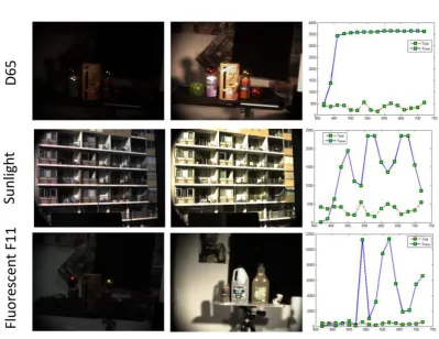
Finally, in Figure 3.8, we illustrate how our method adjusts itself with respect to varying light conditions and scenes. In the figure, in each row we show the pseudo colour images for the initial spectral image, followed by the one acquired using the exposure times yielded by our method and the corresponding time plots. Each row presents different lighting conditions. Note that the imagery acquired using the exposure times computed with our approach exhibit good contrast throughout. The plots also hint to the ability of the method to adjust itself with respect to changing lighting conditions. As before, the red plot corresponds to the random exposure times whereas the blue trace represents the exposure times yielded by our method.
3.4
Summary
Figure 3.8: Results yielded by our method for different lighting conditions (D65, sunlight and fluorescent - F11 ). Left-hand column: Pseudo colour image for the initial imagery taken at random exposure times; Middle column: Pseudo colour image for the hyperspectral image acquired with the exposure times yielded by our method; Right-hand column: Time plots showing the initial and the exposure times
delivered by our approach.
Controllable Automatic Exposure
Adjustment for Cameras
In the previous chapter, we discussed our automatic exposure control technique for spectral cameras using histogram equalization. This technique without loss of any generality can be extended to the trichromatic cameras. In this chapter, we advance our previous approach. Here, instead of applying histogram equalization to each channel, we compute a spectral power image and apply contrast adjustment using histogram equalization, so as to calculate the exposure time for each channel using a minimization approach.
Here, we compute the exposure time based upon a formal stability analysis which assures controllability conditions are satisfied. This, in turn, yields a method which can be applied to a broad range of cameras, with varying architectures and acquisi-tion schemes. Moreover, in order to improve the stability of the method presented here, an error image is used for the exposure time estimation. This error image is the difference between the target image and the spectral power image of the current scene, as yielded by the CIE 1931 photopic function. The method presented here has a number of advantages with respect to that previously discussed. Firstly, its con-trollability is assured. Secondly, the error image used here is an additional constraint as compared to the target image employed previously. Finally, the use of control theory and the error image allows for the introduction of a regularisation term in our cost function. This, in effect, implies that the optimisation problem solved here is different from that explained previously.
The chapter is organised as follows. In Section 4.1 we develop our method for automatically estimating the exposure time. In Section 4.2, we present our stability analysis for the state space representation of the method and elaborate on its control-lability conditions. In Section 4.3 we show the applicability of our method for setting the exposure of a single CCD RGB camera, multiple-CCD multispectral camera and a staring arrays hyperspectral camera. In our experiments, we used a Macbeth Col-orChecker to validate the quality of the results. Finally, in Section 4.4 we conclude and summarize the research presented in the chapter.
4.1
Method
Here we continue from Equation 3.2 and 3.3 given as
I(v,λ) =E(v,λ)Q(λ)Tj , (4.1)
E(v,λ)Q(λ) =V(v,λ). (4.2)
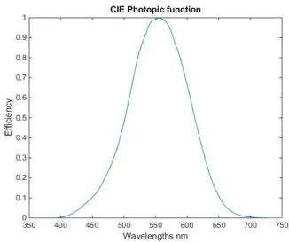
We can estimate the exposure time by comparing the image yielded by the current exposure time setting, with respect to an “ideal” target image. Also, recall that, the luminous flux of light sources are based upon the CIE Photopic function Stiles and Burch [1955]. CIE photopic function depicts the spectral sentsitivity response of human visual system to brightness. The CIE photopic response is presented in figure 4.1. This function is a smooth one across the spectral domain and, hence, here we also adopt the notion that the exposure times should not change steeply across adjacent wavelength-indexed bands. At the same time, we also require the method to be stable, assuring convergence. In the following subsection, we present our method to estimate the exposure time. We also present a controllability analysis.
Considering Equations (4.1) and (4.2), the initial image acquired from the spectral camera can be written as:
Figure 4.1: Photopic response function depicting spectral sensitivity of human visual system when exposed to brightness .
Note that spectral images can be viewed as “cubes”, where the x and y axis represent spatial coordinates, and the z axis represents bands in the spectral domain. Having the initial image cube available, we can generate a target image from which subsequent updates can be computed via an optimization approach. To this end, we employ a spectral power image, which is computed making use of the CIE photopic function (Stiles and Burch [1955]) so as to weight the contribution of each spectral band to the power at each pixel. This yields:
ˆ I(v) =
c
∑
j=1λ
∑
∈ΛjV(v,λ)W(λ)Tj , (4.4)
where W(λ) represents the photopic function at channel λ. Please note that our
in well lit environments (Burton et al. [1992]). Similarly, in low-light conditions, a scotopic function can be used. Other choices of functions can be made based on the application domain.
It can be observed that the spectral power image ˆI(v)is obtained by adding the weighted response for each channel. For simplicity, we can write
Y(v,λ) =V(v,λ)W(λ), (4.5)
such that ˆI(v)becomes
ˆ I(v) =
c
∑
j=1λ
∑
∈ΛjY(v,λ)Tj . (4.6)
Assuming N pixels in a single channel, Equation (4.6) can be rewritten in matrix form as follows
ˆ
I =XT, (4.7)
where ˆI = [Iˆ(1), ˆI(2), . . . , ˆI(N)]T and T = [T
1,T2, . . . ,Tc]T are vectors and X is a
matrix defined as
X= hy1, y2, . . . ymi h1Λ
1, 1Λ2, . . . 1Λc
i
(4.8)
where yi = [Y(1,λi),Y(2,λi), . . . ,Y(N,λi)]T for i = 1, 2, ...,m. 1Λj is an indicator
function which results in a binary column vector of lengthmsuch thatΛj is a subset
of [λ1,λ2, . . . ,λm]T and1Λj(˘i) =1 ifλi ∈ Λj and 0 otherwise. Thus, Xcaptures the
combined effect of the irradiance making use of the photopic response per exposure time for each wavelength setΛj.
used as dictated by the application or lighting conditions.
Our histogram equalized image becomes
I =histeq(Iˆ), (4.9)
wherehisteq(·)is the image equalization operator of choice.
To estimate the update in the exposure time, we employ the difference between the input and the target image given by
e[k] =I −Iˆ[k] , (4.10)
where e[k] and ˆI[k] are the error and spectral power images at iteration k,
respec-tively. Note that, in the equation above, and throughout the paper, we opt to use the notation commonly found in time series analysis for the iteration indexing of the variables. We have done this for the sake of consistency with respect to the common treatment of state space analysis in the control literature.
Since the input images are all of the same scene, we can consider the target equal-ized images to be invariant. In practice, these may also be indexed to iteration num-ber in a straightforward manner. For the sake of simplicity, we consider the ideal case and treat I as being devoid ofk. It is worth noting that in many modern cameras, metering methods like centered, spot or matrix metering are used. These methods apply various weighting techniques to different parts of the scene, which can be incorporated effortlessly by the introduction of a per-pixel prior on the difference equation above.
From Equation (4.7), it can be observed that the image values are related to their exposure time as set in the matrixX. As a result, we can use Equation (4.10) to relate the change in the exposure time to the error at iterationkas follows
e[k] =X∆[k] , (4.11)