Rochester Institute of Technology
RIT Scholar Works
Theses
Thesis/Dissertation Collections
5-16-1990
Optimal selection of textural and spectral features
for scene segmentation
Wendy Rosenblum
Follow this and additional works at:
http://scholarworks.rit.edu/theses
This Thesis is brought to you for free and open access by the Thesis/Dissertation Collections at RIT Scholar Works. It has been accepted for inclusion in Theses by an authorized administrator of RIT Scholar Works. For more information, please [email protected].
Recommended Citation
Optimal Selection
of Textural
and Spectral
Features for Scene Segmentation
by
Wendy Rosenblum
A thesis submitted in partial fulfillment of the requirements for the degree of Master of Science
in the Center for Imaging Science in the College of Graphic Arts and Photography of the
Rochester Institute of Technology
May 16, 1990
Signature of the Author _
Genter. for Imaging Science
Accepted by
Coordinator, M. S. Degree Program
College of Graphic Arts and Photography Rochester Institute of Technology
Rochester, New York
CERTIFICATE OF APPROVAL
M. S. DEGREE THESIS
The M. S. Thesis of WendyI.Rosenblum has been examined and approved by the thesis committee as satisfactory
for the thesis requirement for the Master of Science degree
Dr. John R. Schott, Thesis Advisor
Mr. Carl SalvaggIo
Thesis Release Form
Rochester Institute of Technology College of Graphic Arts and Photography
Title of Thesis: Optimal Features
Selection of Textural and for Scene Segmentation
Spectral
I, Wendy 1. Rosenblum, hereby grant permission to the Wallace Memorial Library of R.I.T. to reproduce this thesis in whole or part. Any
reproduction will not be for commercial use or profit.
Signature
Optimal SelectionofTexturalandSpectral Features
for Scene Segmentation
By
WendyI.Rosenblum
Submittedto theCenter forImagingScience inpartialfulfillmentofthe
requirementsforthedegreeof MasterofScienceatthe
Rochester InstituteofTechnology
Abstract
A study is described in which optimal textural and spectral features are
selected for scene segmentation. A set of 46 textural features and 3 spectral
features were available for image classification. A method was developed
which used a thresholded separability measure to select the best features for scene segmentation. The measure was based based on the Mahalanobis distance between class means.
The optimal feature selection process was applied to a variety of images and classification results using 4 features ranged from 91% to 97% with
independent data sets. The use of the thresholded Mahalanobis-like distance for optimal feature selection was compared to the more common
thresholded divergence separability measure and was found to choose features which were equally good for classification. The Mahalanobis-like
Acknowledgements
The author wishes to thank the many people who have made this project
possible. The author is thankful to Denis Robert who began this project. Special thanks are due to Sharon Cady and Ranjit Bhashkar for their assistance in making
Denis'
computer code more friendly, Eugene Kraus who made the computer code run more quickly and correctly, and Rolando Raqueno for his tremendous debugging skills. Thanks also to Dr. Schott for
good ideas when they were needed most and to Carl Salvaggio for his
endless patience and good humor. Thanks to Jonathan Bannister for providing a firm deadline, and finally, to my parents, William and Vasha
Rosenblum for their encouragement and patience which made it easier for
Dedication
This work is dedicated to the graduate classes of 1989 - ?. Their wide
Table of Contents
List of Figures
List of Tables
1.0 Introduction 1
2.0 Historical Background 2
2.1 Classification of Images 2
2.2 Information in an Image 2
2.3 Tone and Texture 3
2.4 Characterizing Texture 4
2.5 Calculation of Features 6
2.5.1 Angles 6
2.5.2 Window Sample Size 7
2.5.3 Spectral Band Selection 9
2.5.4 Quantization 9
2.6 Textural Features 11
2.6.1 First Order Statistics Features 11
2.6.2 Co-occurrence Features 11
2.6.3 Run Length Features 14
2.7 Classification Theory 16
2.8 Classification Using Features 19
2.9 Summary of Textures 21
3.0 Optimal Feature Selection 22
3.1 Commonly Used Separability Measure 23
3.2 Separability Measure Using the Mahalanobis-like 25 Distance Measure
3.3 Feature Selection 26
3.4 Distance Measure Based on the Mahalanobis Distance 27
3.5 Selection Criterion for Features 29
3.6 Thresholding Distance 30
3.7 Pre-Screening the Features 36
3.7.1 Pre-Selection Approach #1: Correlation Analysis 37
3.7.2 Pre-Selection Approach #2: Eigenvector Criteria 39
4.0 Experimental Process 41
4.1 Description of Images Used 41
4.2 Training Samples for the Classification 46
4.3 Calculation of the Textural Features 48
4.5 Selection of Optimal Features 50
4.6 Dependent and Independent Data Sets 50
4.7 Calculation of Textural Images for Use in a Full 51 Scene Classification
5.0 Results 53
5.1 Comparison of the Two Pre-Selection and Two 53 Optimization Methods
5.1.1 Pre-Selection of Features 53
5.1.2 Optimal Feature Selection 55
5.1.3 Selecting the Number of Features for Classification 64
5.1.4 Optimal Features 65
5.1.5 Classification Results 67
5.2 Classification of the Secondary Images 71
5.2.1 Pre-Selection of Features 71
5.2.2 Optimal Features Selection 73
5.2.3 Classification Results 74
5.2.4 Comparison of Features for the Primary 76 and Secondary Images
5.3 Full Scene Classification of the Primary Images 77
5.3.1 Textural Images 78
5.3.2 Full Scene Maximum Likelihood Classification 78
5.3.3 Random Classification of the Primary Images 81 5.3.4Classification Including More Features 84 5.4 Classification Using Different Sized Windows 85 5.5 Classification Accuracy vs. the Separability Measure 91
5.6 Robustness of the Separability Measure 93
5.7 Random Selection of Features 94
5.8 Classification Using Only Textural Information 96 5.9 Classification Using Only Spectral Information 98 5.10 Divergence as a Feature Selection Criterion 99
6.0 Conclusions 104
6.1 Improving the Optimal Feature Selection Process 104
6.2 Comparison to the Divergence Measure 105
6.3 Robustness of the Separability Measure 105
6.4 Robustness of the Textural Measures 106
7.0 Recommendations for Further Research 107
Appendix A List of Features 111
Appendix B Feature Formulas 113
Appendix C Optimal Feature Lists 121
Appendix D Confusion Matrices for Dependent Data 125
Appendix E Divergence Measure Dependent Data 128
Appendix F Histograms of Separability Measures 130
List of Figures and Graphs
Figure 1 Angular dependence 6
Figure 2 Window size 8
Figure 3 Band selection 9
Figure 4 Quantization 10
Figure 5 Gray-tone co-occurrence calculation 13
Figure 6 Run length matrix calculation 15
Figure 7 Class histograms for feature x 17
Figure 8 The maximum likelihood decision boundary 18
Figure 9 Statistical distances 28
Figure 10 Distance between classes 29
Figure 11 The divergence matrix 33
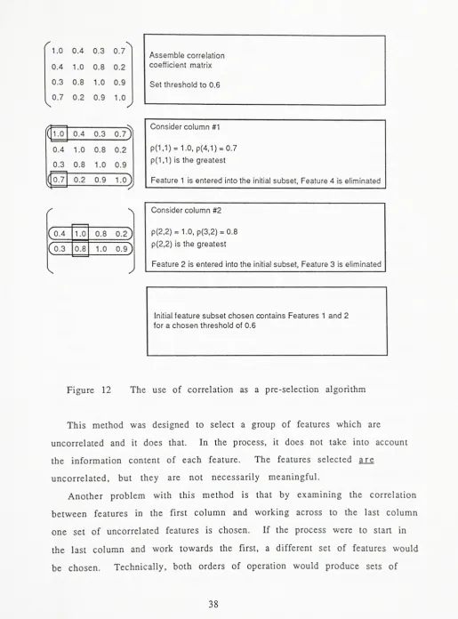
Figure 12 The use of correlation as a pre-selection algorithm 38
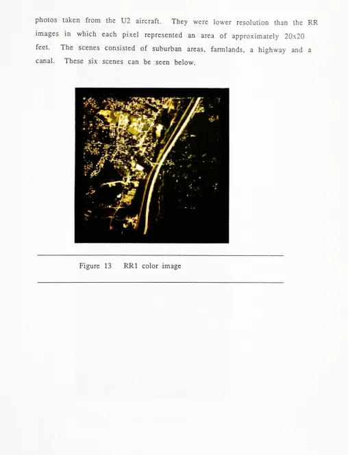
Figure 13 RR1 color image 42
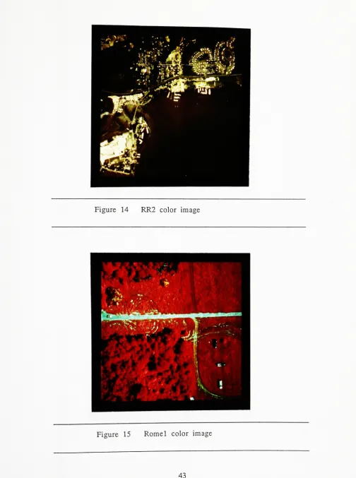
Figure 14 RR2 color image 43
Figure 15 Romel color image 43
Figure 16 Rome2 color image 44
Figure 17 U24 color image 44
Figure 18 U21 color image 45
Figure 19 Training samples for textural features 47
Figure 20 Shrunken training sample 51
Figure 21 RR1 classified image 79
Figure 22 Romel classified image 79
Figure 23 U24 classified image 80
Figure 24 Romel 13x13 classified image 90
Graph 1 New optimization with eigenvectors for RR1 56 Graph 2 New optimization with correlation for RR1 56 Graph 3 Old optimization with eigenvectors for RR1 57 Graph 4 Old optimization with correlation for RR1 57 Graph 5 New optimization with eigenvectors for Romel 58
Graph 6 New optimization with correlation for Romel 58 Graph 7 Old optimization with eigenvectors for Romel 59 Graph 8 Old optimization with correlation for Romel 59 Graph 9 New optimization with eigenvectors for U24 60
[image:11.537.25.518.56.717.2]List of Tables
Table 1 The 15 pre-selected features 54
Table 2 Average classification for 2-6 features 62
Table 3 Four optimal features from eigenvectors 66 Table 4 Classification accuracy for 4 features 67
Table 5 Confusion matrix for RR1 69
Table 6 Confusion matrix for Romel 69
Table 7 Confusion matrix for U24 69
Table 8 15 pre-selected features 72
Table 9 Four optimal features from eigenvectors 73
Table 10 Classification accuracies for 4 features 74
Table 11 Confusion matrix for RR2 74
Table 12 Confusion matrix for Rome2 75
Table 13 Confusion matrix for U24 75
Table 14 Classification of secondary images with primary features 77
Table 15 Color key for classified images 80
Table 16 Random classification of RR1 81
Table 17 Random classification of Romel 82
Table 18 Random classification of U24 82
Table 19 Random classification of RR1 6-band 85
Table 20 4 features for different sized windows 87
Table 21 Features selected from each size window set 87 Table 22 15 features from different window sizes 88 Table 23 Color key for the classified images 90
Table 24 Random classification of Romel 91
Table 25 Robustness of the separability measure 93
Table 26 Random selection of features 95
Table 27 Classification using spectral data 98
Table 28 Classification with 2 separability measures 101
1.0 Introduction
A fundamental part of remote sensing is the segmentation of images into areas containing different land cover types. This task is usually
performed by computer and research over the years has led to many
algorithms which extract textural information from the images to improve the classification of the image.
Two fundamental types of information have been used in
classification: spectral information and textural information (derived from
the pixel to pixel variation within a single spectral band). Studies
performing classification of images with either feature set were able to
provide good results and the accuracy of classification usually improved
when a combination of features was used.
Continued study of classification and the information contained within an image has resulted in hundreds of textural feature algorithms.
Of course not all of them are needed for good classification, so methods of
selecting those best suited for classification has become necessary. These
methods were most often applied to hyperspectral images to select the best
spectral bands for classification.
One of the optimization methods was modified in this study in an attempt to improve its performance. The changes made in the optimization process allowed it to choose a better set of features. The result was a
significantly higher classification accuracy than that which could be
obtained with the features chosen by the original optimization method.
A study of the robustness of the feature selection process was also
included in this study by analyzing three sets of images which differed in
film type and resolution. The optimal features selected for each set and the
classification accuracies which could be achieved for each image provided information about the robustness of the feature selection method.
The results of this study show that very few features are needed to
achieve high classification accuracies after which the addition of more
features did not necessarily increase the classification accuracy. The features which were chosen most often were spectral bands and simple
2.0 Historical Background
2.1 Classification of Images
Classification of an image relies on the information contained within
the image. The information contained in an image can be represented by features where each features is a description of some aspect of the
information in the image. This might be a description of the spectral
characteristics of an area or some aspect of the texture of the area.
All of the features can be combined to form the feature vector of a class
and since the information contained in each class is different, the feature
vectors will be different. These differences make it possible to distinguish between classes such as trees, grass or urban areas since the different features values can be used by a classification algorithm to segment the
2.2 Information in an Image
The human visual system uses three types of information to recognize
objects: spectral, textural and contextural information. Spectral
information describes the information in different spectral bands such as
the redness, greenness and blueness of an image. Textural information describes the brightness variations from spot to spot within one spectral
band and might allow us to distinguish between two objects which are the
same color but differ in texture. Contextural information helps us to
identify an object based on its surroundings. It might help us distinguish a
high school from another building because of the school's proximity to a football field and track (Haralick and Shanmugam, 1974).
The features contained in a feature vector attempt to describe the same
and context (Landgrebe, 1976). This study will be concerned only with
calculated descriptors of spectral and textural information.
2.3 Tone and Texture
The spectral values, or tones, of an area are linked to the texture of that
area; they are not independent (Haralick, 1979). Texture is an extension of the tonal information since it is a description of the spatial distribution and
spatial dependence among the gray tones. A texture image J can be thought of as a transform from one band of a spectral image I in which
J(i,j) is a function of I(i,j) and neighboring pixels (Haralick, 1979).
The texture of an area can be described as fine, coarse, smooth,
granulated, rippled, mottled, irregular, random, lineated or hummocky.
Each adjective translates into some property of tonal variation (Haralick,
1979). When using texture features in classification, each texture must be
assigned an algorithm. This algorithm will produce a number which a
computer can recognize as representing the texture type (Wiersma and Landgrebe, 1976).
The textures in an image can be analyzed either by the primitives that
make up the texture, or the arrangement of those primitives. The simplest
texture primitive is a single pixel with its gray tone property. The next
most complicated primitive is a connected set of pixels homogeneous in
tone. More complicated textures are made by the repetitive placement of
these and other primitives to form a pattern (Haralick, 1979).
Some texture feature algorithms try to recognize the primitives making
up the pattern while others try to identify the pattern composed of some
primitives. An example of searching for the primitives might be to
measure the average tone, or minimum and maximum tone of the region.
Measuring the number of edges in the area would be a way of identifying
2.4 Characterizing Texture
There are many ways of characterizing the texture of an area. All of
these methods describe different ways to extract information about the
image from the order in which the pixels are placed. A few of these
methods as described by Haralick (1979) are listed below.
1. First order statistics: This method described the texture using simple statistical measures such as the mean value of a group of pixels, the
standard deviation, or the frequencies of occurrence for a given gray tone within the group (Haralick and Shanmugam, 1974).
2. Autocorrelation: This is a measure of the correlation between
neighboring pixels in an image. It describes the size of the tonal
primitives which is related to the coarseness of the texture.
3. Optical transforms: These measure the two-dimensional frequency
characteristics of an image. An example of using optical processing to
characterize texture is to measure the Fraunhofer diffraction pattern over small regions of the image. It measures the characteristics of an image in
the frequency domain rather than in the spatial domain.
4. Digital transforms: These take advantage of the fact that frequency is
related to texture. The image is transformed to some new coordinate system
related to frequency by a Fourier or a Hadamard transforms.
5. Textural edgeness: These use an edge detector to measure the number of
edges contained in a group of pixels. The values will increase with rougher textures. The quick Roberts gradient is often used as a measure of these
6. Structural elements or morphology: These use a matching procedure to
detect regularly shaped primitives in an image. They generates a new binary image by erosion and/or dilation of shapes in the original image by
defined structural elements.
7. Co-occurrence: These examine the frequency with which pixels of a
given gray level occur next to each other at a given angular orientation. There are many different features which can be calculated from that
information. They characterize the spatial inter-relationships of the gray
tones, but they do not capture the shape aspects of the texture primitives.
8. Run lengths: These measure the number of times a certain length of
collinearly occurring pixels of the same gray level occur within a window. As with co-occurrence, there are many different features which can be
calculated from the information. It is often a good indication of texture, but can be time consuming to calculate
9. Auto regressive functions: These use linear estimates of a pixel's gray
tone given the gray tones in the neighborhood surrounding the pixel to
characterize texture. They exploit the linear dependence which one pixel has on its neighboring pixels to model texture.
Another sets of features was defined by Weszka and Rosenfeld (1976)
based on other features. The features are made up by functions such as the
average or standard deviations of a feature calculated over all sampling
angles or features computed over a series of distances between pixels.
The list of textural features above describes 9 different measures of
texture. Only 5 of these will be implemented in this study to keep the
number of features calculated to a reasonable size. The features which will be used will be first order, co-occurrence and run length statistics, an
edgeness measure and a contrast measure. All of the features which were
chosen for analysis in this study are listed in Appendix A. The formulas for
2.5 Calculation of Features
There are many problems that arise due to the nature of the textural
feature calculation. A textural feature tries to characterize the spatial
distribution of certain gray level pixels. When the lighting conditions
change or the image is digitized, the distribution of gray levels may
change, changing the value of the calculated feature.
Some textural features are dependent on the angle of the object. If the
same texture occurs at a different angle in two images, the value calculated
may be different even though they show the same texture.
The window over which the feature is calculated is also important. If
the window doesn't even cover one primitive, how can it measure the texture which is made up of the primitives? All of these problems make classification by texture difficult, and the problems and their consequences
are described below.
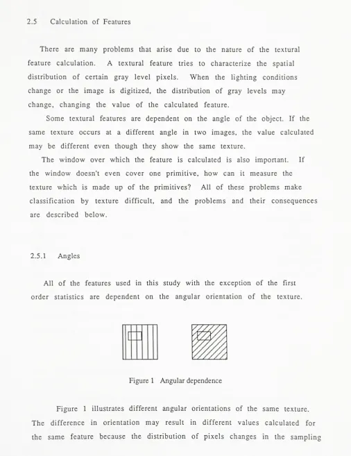
2.5.1 Angles
All of the features used in this study with the exception of the first
[image:19.537.17.524.46.704.2]order statistics are dependent on the angular orientation of the texture.
Figure 1 Angulardependence
windows.
Angular textures are very useful for distinguishing areas with a strong
angular orientation from other areas with different or no angular
orientation. Unfortunately, it also means that if an image were rotated, the feature calculated on the same texture might result in a different value.
In order to retain robustness at any angular orientation of the image,
the average of the feature values calculated over four different angles (0, 45, 90, 135) may be taken as the value of the feature (Haralick et al.,
1973). The range may also be calculated to determine whether there was a
large difference between the feature values calculated at the different
angles which would indicate a strong angular dependence in the scene.
Some information is lost in the combination of angular calculations, but it is hoped that enough information is retained in the average and range
measurements to make classification possible.
Using the average and range of angular measurements also simplifies the classification of complex scenes. Without averaging over angles, roads
that occur at different angles would appear to be from different classes.
The initial training areas would have to be outlined for roads occurring at 0, 45, 90, and 135 since each would produce different feature values and
appear to be from different classes. By using the average and range of the
angular features instead of the individual angle values, a class of roads can be trained for without regard for the angle at which they occur. The
results of the classification should then find all roads, not just those occurring at a specific angle.
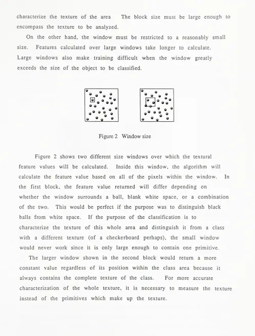
2.5.2 Window Sample Size
The window size over which the textures are calculated determines how
many combinations of pixels will be examined in each feature calculation. A very small window will cover only a few pixels and the texture algorithm
characterize the texture of the area The block size must be large enough to
encompass the texture to be analyzed.
On the other hand, the window must be restricted to a reasonably small
size. Features calculated over large windows take longer to calculate.
Large windows also make training difficult when the window greatly
exceeds the size of the object to be classified.
9
a e
9 9 9 9 9
9
a 9
9 9
9 9
9 Jo
9 9 9
^9
0 99
9
[image:21.537.25.524.37.695.2]9 8 9
Figure 2 Windowsize
Figure 2 shows two different size windows over which the textural
feature values will be calculated. Inside this window, the algorithm will
calculate the feature value based on all of the pixels within the window. In the first block, the feature value returned will differ depending on
whether the window surrounds a ball, blank white space, or a combination of the two. This would be perfect if the purpose was to distinguish black balls from white space. If the purpose of the classification is to
characterize the texture of this whole area and distinguish it from a class
with a different texture (of a checkerboard perhaps), the small window would never work since it is only large enough to contain one primitive. The larger window shown in the second block would return a more
constant value regardless of its position within the class area because it always contains the complete texture of the class. For more accurate
characterization of the whole texture, it is necessary to measure the texture
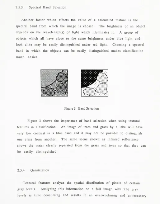
2.5.3 Spectral Band Selection
Another factor which affects the value of a calculated feature is the
spectral band from which the image is chosen. The brightness of an object depends on the wavelength(s) of light which illuminates it. A group of
objects which all have close to the same brightness under blue light and look alike may be easily distinguished under red light. Choosing a spectral band in which the objects can be easily distinguished makes classification
[image:22.537.8.523.49.705.2]much easier.
Figure 3 Band Selection
Figure 3 shows the importance of band selection when using textural
features in classification. An image of trees and grass by a lake will have
very low contrast in a blue band and it may not be possible to distinguish
one class from another. The same scene shown as infrared reflectance
shows the water clearly separated from the grass and trees so that they can be easily distinguished.
2.5.4 Quantization
Textural features analyze the spatial distribution of pixels of certain
gray levels. Analyzing this information on a full image with 256 gray
amount of information. To simplify the process and reduce the amount of
data to a manageable set the images are usually quantized to a lower
number of gray levels before textural features are calculated (Haralick and Shanmugam, 1974).
All textural features are calculated as a function of the gray levels
within the window of pixels. By reducing the number of gray levels, the
time it takes for a feature to be calculated would be reduced from 256
calculations to only 32 (or the number of gray levels after quantization).
This saves a great deal of time when a feature must be computed over an
entire image.
iip
::-:-::
Figure4 Quantization
Figure 4 illustrates the quantization of an image. Some information will
be lost due to quantization because of the loss of detailed gray level
information. The gains in speed of calculation and normalization of the
images should offset some of that loss.
The method used for quantization included two steps. First the image
was histogram equalized so that there was an even distribution of gray tones in the image. The gray levels in the image were then divided equally into the number of gray levels specified for quantization. For example, an
original image with 256 gray levels would first be histogram equalized,
then for a 32 level quantization, 8 gray levels would be placed in each bin
(8x32=256).
[image:23.537.21.523.43.725.2]the imagery. Slight differences in the appearance of images caused by
different lighting, lenses, film processing or digitizing will be much less
noticeable after quantization. The small differences in the original images
will be less likely to cause different values for the same textural features if
the images are quantized before the features are calculated (Haralick and
Shanmugam, 1974).
2.6 Textural Features
There are several different types of textural features used in this study:
a discussion of the calculation of three types follows. In each calculation,
the parameters discussed in sections 2.5.1
-4 play an important role.
For all of the features calculated, the images were quantized to 32 gray
levels. For those textural features which compare two pixels a distance d
apart, the distance was always one so that neighboring pixels were
compared.
2.6.1 First order Statistics Features
First order textural features measure the basic statistical information
about a group of pixels. They are calculated over a specified size group of
pixels, usually a square block although any shape or size group may be
specified. The features, such as the mean brightness or variance, are
computed over the block of pixels (Weszka and Rosenfeld, 1976)
2.6.2 Co-occurrence Features
One way to measure the spatial distribution of gray tones is by using a
p-- with
which two pixels with separation d occur in the image, one with
gray tone i and the other with gray tone j. The relative frequencies are
calculated over four angles: 0, 45, 90 and 135.
This matrix will be symmetric because each occurrence of the two gray
levels is actually counted once for the angle specified and again for that
angle plus 180. For example, when calculating the occurrence at 0, it
would count the specified pair whether it occurs with i on the right and j
? E2 ? cn ED D ess DB ? H
?
B
B .H 1
B
e 1? a ? 0
? ?D n 3 D D EJ ? ?
B
D 0 0 D s 0 E3 0 ? H? 0 ?
u 0
?
D S
0 1 2
1 2 2
2 2 0
? 0
0 2
2
2
D 0 D n
? 0 2 0 D
?
0 1 0
0 2 0 2 1 2 1
[image:26.537.13.523.45.705.2]0 2 0 0 1 2
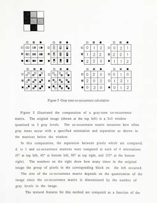
Figure 5 Graytoneco-occurrence calculation
Figure 5 illustrated the computation of a gray-tone co-occurrence
matrix. The original image (shown at the top left) is a 3x3 window
quantized to 3 gray levels. The co-occurrence matrix measures how often
gray tones occur with a specified orientation and separation as shown in
the matrices below the window.
In this computation, the separation between pixels which are compared, d, is 1 and co-occurrence matrices were computed at each of 4 orientations
(0
at top left, 45 at bottom left, 90 at top right, and 135 at the bottom
right). The numbers on the right show how many times in the original
image the group of pixels in the corresponding block on the left occurred.
The size of the co-occurrence matrix depends on the quantization of the
image since the co-occurrence matrix is dimensioned by the number of
gray levels in the image.
values in the co-occurrence matrices. As changes occur in the texture
contained in the window over which the co-occurrence matrix is
calculated, the values within the co-occurrence matrix will change.
Features calculated as a function of the co-occurrence matrix should reflect
these differences making it possible to discriminate between classes with
different textures.
Haralick (1979) found a wide range of images, including satellite
images, tissue samples and micrographs of sandstone, where the gray tone
co-occurrence carried much of the texture information. 28 features based
on gray level co-occurrence have been proposed by Haralick, some of
which are described in Appendix B.
2.6.3 Run Length Features
Another way to describe the spatial distribution of gray levels is by
using run lengths. It is similar to the calculation of co-occurrence
features but in this case, the frequency of connected pixels of a certain
gray level is computed (Galloway, 1975).
As with the co-occurrence features, a matrix is formed containing the
probability frequency
p-, of a run of pixels having gray level i and length
1. Each position in the matrix contains the number of times 1 pixels of gray
level i occurred in a straight line. This matrix is computed for four
different angles, 0, 45, 90 and
135
to capture any angular dependencies
in the data. Note that in this case the matrix is neither symmetric nor
square. An illustration of the run length matrix calculation is shown
? ? m Mil
0 EQ 0?.W
"
? ? B 3
0
1
i
1
i
? ? ?D
? D ? ? 0 D D a 0 a n
0 0 0
0 0 0 0 0 0 0 0 0 E3 D
? 3 0 0
EJ 3 1 0
3 0 0
? 3 0 0
0 3 0 0
E 3 0 0
? 3 0 0
ej 3 1 0
a 3 1 0
a 3 0 0
0 3 1 0
3 1 0
Figure 6 Run length matrix calculation
Figure 6 illustrates the computation of a run length matrix. The
original image is the same as that for the co-occurrence calculation. The
matrices were computed at each of 4 orientations (0 at top left, 45 at
bottom left, 90
at top right, and 135 at the bottom right). The numbers on
the right show how many times in the original image the group of pixels in
the corresponding block on the left occurred.
The textural features are then computed as a function of the entries in
the run length matrix. Different formulas (described in Appendix B) can
either emphasize the long runs, the short runs, or different distributions
of run lengths so that classes with different textures may be distinguished
2.7 Classification Theory
Classification is the process of segmenting an image into separate
classes. Supervised classification begins with a sample from each class of
grass, trees, suburbs, and analyses the statistical distribution of the
elements in each class. From that information, the classification algorithm
reaches a decision about how to assign areas outside the class samples to the
appropriate classes. Classification is a decision making process which uses
statistical decision theory to make intelligent estimate of which class a
pixel belongs to (Schowengerdt, 1983).
Supervised training is used to identify an area representative of each
class for the classification algorithm. Homogeneous areas are outlined for
each class, and these are referred to as the training areas for the class.
Each training area should contain pixels in only one class, but the range of
variability for the class must be covered. For example, training areas may
need to be outlined for both dark and light water if the class being trained
is water.
Schowengert (1983) recommends that at least 10 to 100 pixels be
included per training class with more pixels for those classes with higher
variability. To achieve a good estimate of the class distributions, at least 100
pixels were included in each training sample. The number of features
which were being used increased the number of degrees of freedom in the
statistical analysis, requiring more samples for a good estimate of statistical
parameters.
Histograms showing the distribution of pixels within a class can be
class 1
p(xli) class 2
j feature x
Figure 7 Class histograms for feature x
Figure 7 illustrates the distribution of values of feature x in two classes.
Each curve is normalized to have an area of 1.0. Feature x may be a
measure of a spectral value, or any of the features mentioned above. It is
some measurement made on the pixels in the image. The histograms show
the distribution of values calculated for that feature in each of the class
training areas. These relative frequency histograms are assumed to
approximate the probability density functions of the classes.
The probability of finding a feature value of j given that we are
sampling from class i (where i, in this case, may equal 1 or 2) is given on
the Y axis as p(xli). This assumes that the feature values are normally
distributed in each class. The discriminant function is defined as the
probability of a pixel belonging to class i given that it has a feature value x
or p(ilx).
P(ilx)
P(xli) P(i)
p(x)
(D
where p(i) is the a priori probability that class i exists in the image
p(x) is the probability of finding a pixel from any class at location x, a normalizing constant
Assuming that each class has an equal probability of occurring in the
each class since it is a normalizing factor, so the discriminant function is
simple a calculation of p(xli) for each class.
Maximum likelihood classification compares the values of the
discriminant function for a feature value x calculated for each class and
assigns the pixel to the class which produced the highest value. For
example, the pixel with a feature x value of j as shown in Figure 7 would be
assigned to class 1 using a maximum likelihood classification. The value of
the discriminant function is greater for class 1 than class 2 (i.e. p(xll) >
p(xl2)), so the pixel is assigned to class 1: it is more likely to belong to that
class.
The decision boundary for classification corresponds to the point at
which the two distributions cross as shown in Figure 8.
class 1
p(xli) / "i class 2
^h
^^
)dx feature x
Figure 8 The maximum likelihood decision boundary
A pixel would be classified as class 1 for feature values less than
dx
sincethe value of the p(xll) is greater than p(xl2) for all those values of x. For
values of x greater than dx, it would be classified in class 2 since the value
of the p(xl2) is greater than p(xll).
The total error in this classification is represented by the overlap of the
distributions as illustrated by the black region in Figure 8. Note that
moving the decision boundary in either direction would increase the error,
so error is minimized by placing the decision boundary where p(xll) =
p(xl2).
This example has illustrated classification using only one feature to
multivariate case so that all of the features defined above may be used. The procedure remain the same, but the math is more complex since it involves
matrices instead of single values. Instead of a feature value x, there is a
vector X. which is referred to as the feature vector. Each pixel has a set of
feature values associated with it which will be used to estimate which class
it belongs to.
Assuming a normal distribution of feature values in each class and
equal prior probabilities, the decision function can be written as
(Schowengert, 1983).
P(Xli) = -'
k.
i-2 2
(2ti) IZ.'
exp [-
\
(X-M.)T z;1
(X
-M.)] (2)
i
P(Xli) is the probability of finding the value X when sampling from class i
X. is the pixel's feature vector
M is the mean vector for class i
E; is the kxk covariance matrix for class i
k is the number of features used
The pixel to be classified is assigned to the class for which the probability is
highest. The probability function is now p(XJi) and the decision boundary
(for k features) is a k-dimensional surface instead of a single point.
2.8 Classification Using Features
The calculated textural feature value will change according to the
texture of the area over which the feature is calculated. These differences in feature values between different classes make it possible to segment the
image. These differences may be obvious when we think of spectral
(equal amounts of red, green and blue). Trying to distinguish between two
classes with respect to textural features may not be so obvious when they
are measures such as the difference contrast or angular second moment
average.
Wiersma and Landgrebe (1976) calculated four basic co-occurrence
features on two classes to illustrate how textural values will change from
class to class. The values obtained for the features demonstrate that it is
possible to distinguish different classes using textural measures.
The classes used were water (a flat smooth surface) and an agricultural
area (a course patchwork pattern of fields). The four features calculated
were angular second moment, contrast, correlation and entropy as defined
in Appendix B. The means of those texture features calculated with a 15x15
window over four angles were
agric. water
ASM 0.0494 0.7641
Contrast 2.6692 0.9481
Correlation 0.5140 0.5458
Entropy 1.4584 0.3270
The angular second moment is a measure of the homogeneity of the
image. Water has a higher value for this feature than the course pattern of
fields because the water is more homogeneous. Contrast is a measure of the
degree of local variations in the image. The calculated value for this
feature is higher for the agricultural area than for the water. This shows
that the fields have more local brightness variation. Correlation measures
the gray tone linear dependencies in the image. This feature is
approximately the same for both water and the fields. This may be
because over a 15x15 pixel area there is high correlation between
neighboring pixels even though the overall pattern is course. Finally,
entropy is a measure of the variability of the image. As with Contrast, the
higher variability in that class compared to the class of water (Wiersma
and Landgrebe, 1976).
From the information above, it can be seen that the feature values
calculated for each class represent the texture within that class. By using
textural feature values in the feature vector for each class, correct
classification can often be successfully accomplished.
2.9 Summary of Textures
The development of textural features and their use in classification has
been described in the previous sections. Haralick, et al. (1973) developed
features based on gray level co-occurrence. Haralick and Shanmugam
(1974) used both those features and spectral information to classify an ERTS
image of the California coastline. The categories for classification included
coastal forest, wood lands, annual grass lands, water bodies, urban areas,
and small and large irrigated fields. They reported that up to 70% of the
image was classified correctly based only on textural features compared
with 74 to 77% accuracy using only spectral features. With textural and
spectral features combined, up to 83% of the image was classified correctly.
Galloway (1985) developed a series of features based on run lengths.
Using these to classify an image, she reported 83% accuracy. Lendaris and
Stanly (1969) reported 90% accuracy when using features obtained by
optical processing methods in classification. Many textural features have
been defined and have been used successfully in classification to achieve
classification accuracies between 75 and 90%.
The classification accuracies obtained with each method can not be
compared directly since the experimental method used to achieve each of
them is not known. They do show that classification is possible with
textural features, and that a combination of textural and spectral features
can result in higher classification accuracies than could be achieved with
3.0 Optimal Feature Selection
Over the past few decades, work has progressed to increase the number
of ways to extract information from an image by defining textural feature
algorithms. As a result, a new problem must be addressed: how to select a
manageable and meaningful set of information from the mass that is
available?
There are 27 textural features defined in Appendix A for use in this
study of which 21 are dependent on angle. After average and range
calculations on the angularly dependent features, 46 textural feature
values are calculated. Adding three spectral bands, there are 49 feature
values available for use in image classification
-too many! In order to
handle this excess of information, several methods of data reduction have
been developed.
One of the easiest methods of data reduction which has been used with
spectral information is principal components analysis. This is a technique
used for removing or reducing spectral correlation (Schowengerdt, 1983).
It forms a new k-dimensional set of data from a linear combination of the
original k bands of data.
The new bands are uncorrelated and ordered by decreasing gray level
variance. Usually only a few of the transformed bands are necessary for
classification, so this method reduces the data needed for classification as
well as removing correlation between bands.
This method is inappropriate for use with textural features because it
would require the calculation of entire textural images (very time
consuming) before the transformation could be made. A method of feature
selection would be better than a transformation.
The main goal of feature selection is to select a subset of m features out
of the total set of N features (m<N) without significantly degrading the
classification system. The number of features used in the classification
should still give a minimal probability of mis-classification (Fu, 1976).
and since many of the features are highly correlated the removal of
redundant information will not affect the classification power. Also,
features which do not add to classification accuracy represent a cost since
with a maximum likelihood classifier, the time needed to make a calculation
increases quadraticly with the addition of features (Richards, 1986).
There are many feature selection algorithms available, but all are
characterized by a search procedure, a selection criterion, and a stopping
criterion (Queiros and Gelsema, 1984). In the search procedure, some
measure of the classification ability or separability of classes is made for
each combination of m features out of N. The subset with the most potential
for correct classification is selected. The stopping criterion analyzes the
effect of including additional features. The improved accuracy (if any) is
weighted against the extra computation necessary for another feature and
is used to decide whether or not the addition is worthwhile. If it is not, the
process is stopped. These three simple steps should lead to the selection of
the best features for the classification of the image. The separability
measures used in this study are described below.
3.1 Commonly Used Separability Measure
Richard (1986) described a way to quantify the separation between a
pair of probability distributions as an indication of the degree of overlap of
the class distributions (the less overlap, the easier the classification). He
states that the distance between class means is not enough since overlap
will also be influenced by the standard deviations of each class.
Divergence is defined in terms of class probability distributions as
described in Section 2.6.
d.. p(Xli)
-p(Xlj) 1In P^) dXjy p(Xlj)
~
(3)
djj
is the divergence between classes i and j p(XJi). p(XJj) are the probabilities of finding thefeature vector X_ when sampling from class i or j
This measure is always positive and d- = d-- (i.e. it is
symmetric).
When the classes can be assumed to come from multidimensional normal
distributions, equation 3 can be rewritten as
1 r i i^i
d = i-Trl (S.-X.)(L. -L.)i+i_Tr
-ij 2 L J J J '
V2
(2"i1-s:1)(M..-Mi)(M..-Mi)T
(4)
E is the covariance matrix for class i or j
M is the mean vector for class i or j
Using this formula, the divergence between two classes using a set of
features can be calculated. The sum of divergences over all class pairs for
the set of features can be used as a measure of the overall divergence; the
feature set which results in the highest sum of divergences should also
result in the greatest separability between classes and the best
classification.
The number of calculations needed to measure divergence depends on
the number of bands to be selected. The total number of calculations is
determined by the number of permutations of the bands to choose out of
15 for an image with 7 classes, the number of calculations would be:
15! 1
4!
(15-4)'
7!
2! (7-2)!. 28665
(5)
For each of these 28665 divergence measures, two matrix inverses must be
computed which can make this method slow to calculate.
Mausel et al. (1990) used the divergence method in the optimal band
selection process to choose the best 4 spectral bands from a set of 8. They
used those 4 bands with a traditional gaussian maximum likelihood
classifier (using the Mahalanobis distance measure) and reported 90%
accuracy in a gaussian maximum likelihood classification.
A transformed divergence measure in the form of equation 6 was
introduced to scale the divergence measure.
td.. = 2000 ij
'.<o
1-exp
V (6)
This transformed divergence measure was developed to emphasize small
changes in divergence resulting from significant changes in class
separability. It also limits the higher values of divergence (to values of
2000 in this case) since large divergence values do not necessarily
correspond to complete class separation with the plain divergence
measure. Using the transformed measure, classification accuracies were
found to reach 92.2% in experiments performed by Mausel (1990).
3.2 Separability Measure Using the Mahalanobis-Like Distance Measure
Another optimization method was developed by Schott et al. (1988) for
the optimal selection of spectral bands from imaging spectrometer data. In
separation of the two classes. It occurs in the exponential part of the
probability equation (2). This distance is defined as
T d.. =
(M.-M.)
E'1(M.-M.)
(7)IJ J v v j V v '
M_i>
M_-are the mean vectors of classes i and j
E is the pooled covariance matrix
This equation assumes equal covariance matrices between all classes. Since
this assumption is not usually true, individual covariance matrices were
used with this measure in the studies by Robert (1989), Schott et al. (1988).
The distance between each pair of classes is measured for a set of
features. The set of features which produces the highest sum of distances is
selected as the best set for classification. In this case, however, the matrix
of separability measures is not symmetric due to the use of individual
covariance matrices in the distance calculations.
This method is faster to calculate since it involves only one matrix
inversion. The results of classifications with the selected features are,
however, slightly worse. Robert (1989) used this feature selection method
on several images and reported classification accuracies between 83% and
91%. The results are believed to be slightly worse because the feature
selection method was not picking an optimal set of features.
3.3 Feature Selection
Two separability measures were outlined in Sections 3.1 and 3.2 for use
in feature selection. Of these two, this study is primarily concerned with
improving the optimal feature selection method developed by Schott et. al
(1988), Robert (1989), and Salvaggio et al. (1990).
achieved by Mausel et al. (1990) because the feature selection method
using the separability measure discussed above in Section 3.2 would not
select the optimal set of features. There are several changes which could
be made in that method which should lead to significant improvements in
the feature selection. These improvements may lead to a feature selection
method which is comparable to the one defined by Richards; having the
advantage of being faster to calculate.
Two steps in the optimal feature selection will be discussed. The first is
the algorithm to select the optimal features. The second is a pre-selection
algorithm to reduce the number of features which the optimization
algorithm has to compare.
3.4 Distance Measure Based on the Mahalanobis Distance
The equation for the Mahalanobis distance is based on the assumption of
equal covariance matrices for all classes. The class covariance matrices
used in preliminary tests failed the likelihood ratio test which determines
whether or not the matrices are approximately equal and can be pooled.
The covariance matrices are usually different for all classes because the
information in each class is different, and since the class covariance
matrices are not likely to be equal, the Mahalanobis distance measure is not
appropriate for measuring the distance between classes.
Richards (1986) defined a distance measure which is similar to the
Mahalanobis distance, but corrected for individual covariances.
d.. =
lnl.l+[(Mj-Mi)x;1(Mj-Mi)j
(g)
E; is the individual covariance matrix corresponding to class i
not used in the feature selection method.
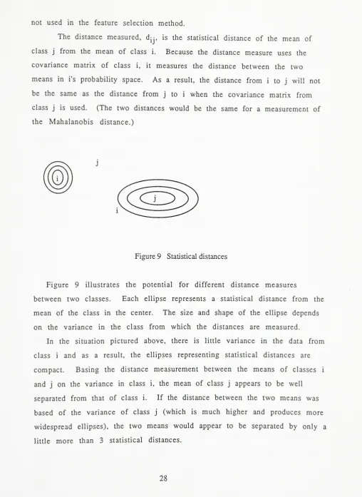
The distance measured, d-, is the statistical distance of the mean of
class j from the mean of class i. Because the distance measure uses the
covariance matrix of class i, it measures the distance between the two
means in i's probability space. As a result, the distance from i to j will not
be the same as the distance from j to i when the covariance matrix from
class j is used. (The two distances would be the same for a measurement of
the Mahalanobis distance.)
Figure9 Statistical distances
Figure 9 illustrates the potential for different distance measures
between two classes. Each ellipse represents a statistical distance from the
mean of the class in the center. The size and shape of the ellipse depends
on the variance in the class from which the distances are measured.
In the situation pictured above, there is little variance in the data from
class i and as a result, the ellipses representing statistical distances are
compact. Basing the distance measurement between the means of classes i
and j on the variance in class i, the mean of class j appears to be well
separated from that of class i. If the distance between the two means was
based of the variance of class j (which is much higher and produces more
widespread ellipses), the two means would appear to be separated by only a
[image:41.537.17.526.34.732.2]3.5 Selection Criterion for Features
The selection of the optimal set of features is based upon the
separability measure described earlier. The distance between all pairs of
class means is measured for a set of features. (Note that because of the
asymmetry in the distance measurements, two distance measures must be
made for each pair of classes.) These distance measures are summed and
the set which produces the highest value should also produce the best
separability between the classes. This should be the best set for
classification of the image.
Assuming a simple case in which the distance from a to b equals that
from b to a, Figure 10 below demonstrates a problem which arises when
choosing optimal features as described above.
Figure 10 Distance betweenclasses
Unfortunately, the highest sum of distances does not always provide the
best separation as illustrated in Figure 10. The group of classes on the left
represent a well separated group. The group on the right is not well
separated, but the sum of distances between class means is greater.
According to the criterion of the selection algorithm, the second group
would be chosen as best for classification although it would be less
effective for separating the classes.
This problem was recognized by Schott et al. (1988), Robert (1989) and
Salvaggio et al. (1990). These studies proposed that an improvement could
be made by assigning weighting factors to the individual Mahalanobis
solution would primarily be used to separate targets from the background
rather than insuring good overall classification. It was designed for target
recognition in a scene, not for overall classification. A new distance
thresholding method which provided better overall separation between
classes as well as requiring no prior knowledge of class separation was
developed in this study.
3.6 Thresholding Distances
To correct for the possibility of selecting a poor set of features as
described above, a distance threshold was developed. The purpose of this
threshold is to prevent one well separated class from inflating the sum of
distances. Without that inflation, a set of features which separates all of
the classes will be chosen instead of a set which separates one class very
well.
The threshold serves the same purpose as the transformed divergence
measure described in Section 3.1. While that formula produces an
exponential scaling, this takes into account how far apart class means need
to be for them to be well separated and uses that distance as a threshold.
The value for the threshold depends on the separability of the classes.
The value calculated determines how many statistical distances apart the
two class means need to be so that the probability of misclassification
between the two is low. This value must be computed for each class because
The probability of finding the mean of class j in a sample from class i is
described as (Schowengert, 1983)
r
1i
t
i 1,1 -T^fM:) 2, (M.-M,)]
P(M.li) =
|
2
I
e"
(9)
"J '
l IE.I 2tc2
|
P(M-i'i) is the probability that the mean of class j belongs to
class i
k is the number of bands which we are trying to
optimize for
E_- is the covariance matrix for class i
M_j is the mean vector of class i
M_i is the mean vector of class j
The equation can then be rewritten as
1_
IE.I 271
k
= e 2 D (10)
where D = [(M.j-Mj)Si*1 (Mj-Mj)] P = PfMjIi)
By taking the natural log of both sides, the equation becomes
ln[P]+-knN+4ln[2*] = -i-D
2
(H)
Multiplying by -2 and adding lnlE^I to both sides gives the equation
D + ln = -2 ln[P] - k
This equation can be modified to the final form belo\
D + ln = -2 In
L27t
(13)
The quantity D+lnlE_jl is the distance between two class means when
individual covariances are used in the calculation. The right hand side of
the equality is the distance which must separate two class means for the
probability of misclassification to be P.
The probability calculated in equation (9) is based on the assumption of
normally distributed variables. Many of the feature values are not
normally distributed for each class, so the value of P is not meaningful in this case. A value of 1.0 x
10" -^
was arbitrarily specified so that the
calculated threshold distance would be greater than the calculated distance between class means in most cases. The threshold distance had to be
greater to prevent the summed distances between class means, the
separability measure, from reaching its maximum value. (If it did, there would be no way to distinguish between different feature set's potential to
segment the scene since many would produce the same maximum value.)
The small value of P chosen was necessary to produce large enough
threshold distances, but the value of the probability was not meaningful
since the assumption of normally distributed variables was violated.
The distance corresponding to the chosen probability can be solved for
since both P and k have been specified by the user. This distance is the threshold for the actual distance between the two classes since the distance
solved for above is the minimum distance needed for good classification.
There are now two distance measures which need to be calculated between two class means: the actual distance as calculated by equation (8)
d.. = In E.
r -i i
+1 (M.-M.) E.1
(M.-M.)l
and the threshold distance from equation (13).
thresh
-21n k_
2k2.
(15)
If the actual distance between the class means is greater than the threshold
distance, the two class means are separated by a greater distance than is
necessary for good classification.
The extra separation is good, but the distance measure for the well
separated means will inflate the value for the sum of all distances between
classes. To prevent that inflation, the actual distance between the class
means is limited to the threshold distance. The ratio of the actual distance
to the threshold distance is computed as in equation 16.
d.. ij
ratio
"thresh
(16)
If the value of this ratio is greater than 1.0, it is set equal to 1.0.
When the thresholded distances have been computed between all class
means for one subset of features, a matrix of values will result as can be
seen in Figure 11.
dll/dt dl2/dt ... dlx/dt
d21/dt d22/dt
dyl/dt dyx/dt
In Figure 11, doi is the distance between the means of classes 1 and 2
using class l's covariance matrix, and
dj2
is the distance between classes 1and 2 using class 2's covariance matrix.
dt
is the threshold distance. If thevalue of any of the ratios is greater than 1.0, its value is set equal to 1.0.
The sum of the values in this matrix is used as the measure of how well a
subset of features separate the class means in the image. All of the class
means will have to be well separated for the sum of the thresholded
distances to reach a high value. The sum of distances is computed for all
permutations of feature subsets from the whole set, so the subset with the
highest summed distance will be chosen as the best features to separate the
classes. The following flowchart demonstrates the steps which have been
Choose a subset of features from the whole set
Calculate the distance between the two class means i and j
in i's probability space
Calculate the standardized distance between any two class means needed for a probability of misclassification, P
Divide the actual distance meaasured between the class means
by the standardized distance. Is the ratio greater than 1.0?
I
NoI Yes
the separation between the two means
is good enough, set the value of the ratio equalto 1.0
Have all combinations of classes been tested for for this set offeatures?
no
Choose a new
i andj
yes
Sum all distances measures computed with this subset of features
Have all subsets been tested
no
ted
ij
yes
Choose a new subset
For this optimal feature selection process, two changes have been made
to the original separability measure by Schott et al. (1988). The first was to
change the distance measure used from the Mahalanobis distance with
individual class covariances to a Mahalanobis-like distance which has been
adapted for the use of individual covariance matrices by the addition of the
InlEjl term. The second change was the implementation of a thresholding
distance which would limit the sum of distances between class pairs for a
set of features. These two changes should improve the selection of features
to provide a more optimal set.
3.7 Pre-Screening the Features
The method described above will select the optimal subset of features for
the classification of an image. If all combinations of 5 features out of the
49 defined in this study were tested, there would be 1,906,884 combinations
of features to test. By reducing the number of features from 49 to a set of
15, the combinations of 5 features would be reduced to only 3,003. The
number of features to calculate would be reduced by a factor of 635, and so
would the time needed to compute and compare the separability of the
feature subsets.
Pre-selection algorithms are not optimal processes, but they try to
reduce the number of features on which the optimization program works.
This will greatly reduce the time spent on feature selection as well. The
pre-selection process serves to eliminate features which are highly
correlated with other features, or those features which do not contain
much unique information leaving only the meaningful,<