High Performance Dimension Reduction and
Visualization for Large High-dimensional Data
Analysis
Jong Youl Choi
∗†, Seung-Hee Bae
∗†, Xiaohong Qiu
∗and Geoffrey Fox
∗†∗Pervasive Technology Institute
†School of Informatics and Computing
Indiana University, Bloomington IN, USA
{jychoi, sebae, xqiu, [email protected]}
Abstract—Large high dimension datasets are of growing im-portance in many fields and it is important to be able to visualize them for understanding the results of data mining approaches or just for browsing them in a way that distance between points in visualization (2D or 3D) space tracks that in original high dimensional space. Dimension reduction is a well understood approach but can be very time and memory intensive for large problems. Here we report on parallel algorithms for Scaling by MAjorizing a COmplicated Function (SMACOF) to solve Multidimensional Scaling problem and Generative Topographic Mapping (GTM). The former is particularly time consuming with complexity that grows as square of data set size but has advantage that it does not require explicit vectors for dataset points but just measurement of inter-point dissimilarities. We compare SMACOF and GTM on a subset of the NIH PubChem database which has binary vectors of length 166 bits. We find good parallel performance for both GTM and SMACOF and strong correlation between the dimension-reduced PubChem data from these two methods.
I. INTRODUCTION
Thanks to the most recent advancement in science and technologies, the amount of data to be processed or analyzed is rapidly growing and it is already beyond the capacity of the most commodity hardware we are using nowadays. To keep up with such fast development, study for data-intensive scientific data analyses [1] has been already emerging in recent years. Including dimension reduction algorithms which produce lower dimensional representation of high-dimensional data, which we are focusing in this paper, various machine learning algorithms and data mining techniques are also the main tasks challenged by such large and high dimensional data problem in this data deluge era. Unless developed and implemented carefully to overcome such limits, techniques will face soon the limit of usability.
Visualization of high-dimensional data in low-dimension is the core of exploratory data analysis in which users want to discover meaningful information obscured by the intrinsic complexity of data, usually caused by its high dimensionality. This task is also getting more difficult and challenged in recent days by the fast increasing amount of data to be analyzed. In most data analysis with such large and high-dimensional dataset, we have observed that such task is no more CPU
bounded but rather memory bounded in that any single process or machine cannot hold the whole data in memory any more. In this paper, we tackle this problem for developing high performance visualization for large and high-dimensional data analysis by using distributed resources with parallel com-putation. For this purpose, we will show how we devel-oped two well-known dimension-reduction-based visualization algorithm Multidimensional Scaling (MDS) and Generative Topographic Mapping (GTM) in the distributed fashion so that one can utilize distributed memories and enable to process large and high dimensional dataset.
In this paper, we start with brief introduction of Multidimen-sional Scaling (MDS) and Generative Topographic Mapping (GTM), which are the dimension reduction algorithms to generate a configuration of the given high-dimensional data into target-dimensional space, and the correlation method we applied to compare outputs from different data visualization algorithms in Section II. Details of our parallelized version of MDS and GTM will be discussed in Section III. In the next, we show our performance results of our parallel version of MDS and GTM in various compute cluster settings and present the result processing up to 100,000 data points in Section IV followed by our closing discussion and future works in Section V.
II. BACKGROUND
There are several kinds of dimension reduction algorithms, such as Principle Component Analysis (PCA), Generative Topographic Mapping (GTM) [2], [3], Self-Organizing Map (SOM) [4], Multidimensional Scaling (MDS) [5], [6], to name a few. Among those algorithms, we focus on MDS and GTM in our paper due to their popularity and theoretical strong backgrounds.
A. Multidimensional Scaling (MDS)
Multidimensional scaling (MDS) [5], [6] is a general term for techniques of constructing a mapping for generally high-dimensional data into a target dimension (typically low dimen-sion) with respect to the given pairwise proximity information. Mostly, MDS is used for achieving dimension reduction to vi-sualize high-dimensional data into Euclidean low-dimensional space, i.e. two-dimension or three-dimension.
Generally, the proximity information, which is represented
as anN×N dissimilarity matrix (∆= [δij]), whereN is the
number of points (objects) andδij is the dissimilarity between
pointiandj, is given for the MDS problem, and the
dissimi-larity matrix (∆) should agree with the following constraints:
(1) symmetricity (δij =δji), (2) nonnegativity (δij ≥0), and
(3) zero diagonal elements (δii = 0). The objective of MDS
techniques is to construct a configuration of the given high-dimensional data into low-high-dimensional Euclidean space, while each distance between a pair of points in the configuration is approximated to the corresponding dissimilarity value as much as possible. The output of MDS algorithms could be
represented as an N ×L configuration matrix X, whose
rows represent each data points xi (i = 1, . . . , N) in L
-dimensional space. It is quite straightforward to compute
Euclidean distance between xi and xj in the configuration
matrixX, i.e.dij(X) =kxi−xjk, and we are able to evaluate
how well the given points are configured in theL-dimensional
space by using suggested objective functions of MDS, called STRESS [7] or SSTRESS [8]. Definitions of STRESS (1) and SSTRESS (2) are following:
σ(X) = X
i<j≤N
wij(dij(X)−δij)2 (1)
σ2(X) = X
i<j≤N
wij[(dij(X))2−(δij)2]2 (2)
where1≤i < j ≤N andwij is a weight value, so wij ≥0.
As shown in the STRESS and SSTRESS functions, the MDS problems could be considered as a non-linear optimiza-tion problem, which minimizes STRESS or SSTRESS funcoptimiza-tion
in the process of configuring L-dimensional mapping of the
high-dimensional data.
B. SMACOF & its Complexity
There are a lot of different algorithms to solve MDS problem, and Scaling by MAjorizing a COmplicated Func-tion (SMACOF) [9], [10] is one of them. SMACOF is an iterative majorization algorithm to solve MDS problem with STRESS criterion. The iterative majorization procedure of the SMACOF could be thought of as Expectation-Maximization (EM) [11] approach. Although SMACOF has a tendency to find local minima due to its hill-climbing attribute, it is still a powerful method since it is guaranteed to decrease
STRESS (σ) criterion monotonically. Instead of mathematical
detail explanation of SMACOF algorithm, we illustrate the SMACOF procedure in this paper. For the mathematical details of SMACOF algorithm, please refer to [6].
Algorithm 1 SMACOF algorithm
1: Z⇐X[0]; 2: k⇐0;
3: ε⇐small positive number;
4: M AX⇐ maximum iteration;
5: Computeσ[0]=σ(X[0]);
6: while k= 0or (∆σ > εandk≤M AX) do
7: k⇐k+ 1;
8: X[k]=V†B(X[k−1])X[k−1]
9: Computeσ[k] =σ(X[k])
10: Z⇐X[k];
11: end while
12: return Z;
Alg. 1 illustrates the SMACOF algorithm for MDS solution. The main procedure of SMACOF is iterative matrix multi-plications, called Guttman transform, as shown at Line 8 in
Alg. 1, whereV† is the Moore-Penrose inverse [12], [13] (or
pseudo-inverse) of matrix V. The N ×N matrices V and
B(Z)are defined as follows:
V = [vij] (3)
vij =
(
−wij ifi6=j
P
i6=jwij ifi=j
(4)
B(Z) = [bij] (5)
bij =
−wijδij/dij(Z) ifi6=j
0 ifdij(Z) = 0, i6=j
−P
i6=jbij ifi=j
(6)
If the weights are equal to one (wij = 1) for all pairwise
dissimilarity, then
V = N
I−ee t
N
(7)
V† = 1
N
I−ee t
N
(8)
where e = (1, . . . ,1)t is one vector whose length is N. In
this paper, equal weights is assumed and we use (8) for V†.
As in Alg. 1, the computational complexity of
SMA-COF algorithm isO(N2), since Guttman transform performs
multiplication of N ×N matrix and N ×L matrix twice,
typically N ≫ L, and computing STRESS value, B(X[k]),
and D(X[k]) also take O(N2). In addition, the SMACOF
algorithm requires O(N2) memory because it needs several
N×N matrices as in Table I. Due to the trends of digitization,
data size increases enormously so it is critical to be able to investigate large data set. However, it is impossible to run SMACOF for large data set under a typical single node
computer due to the memory requirement increases inO(N2).
algorithm via message passing interface (MPI) for utilizing distributed-memory cluster systems in Section III-A .
C. Generative Topographic Mapping (GTM)
Generative Topographic Mapping (GTM) is an unsupervised learning algorithm for modeling the probability density of data and finding a non-linear mapping of high-dimensional data in a low-dimension space. Contrast to the Self-Organizing Map (SOM) [4] which does not have any density model [2], GTM defines an explicit probability density model based on Gaussian distribution. For this reason, GTM is also known as a principled alternative to SOM [2]. The problem challenged by the GTM is to find the best set of parameters associated with Gaussian mixtures by using an optimization method, notably the Expectation-Maximization (EM) algorithm [3].
More specifically, The GTM algorithm is to find a
non-linear manifold embedding of user-defined K latent discrete
variables zk, usually form a rectangular grid, in low L
-dimension space, called latent space, such that zk∈RL(k=
1, ..., K), which can optimally represent the given N data
points xn ∈ RD(n = 1, ..., N) in the higher D-dimension
space, called data space (usually L ≪D). This is achieved
by the three steps: First, mapping the latent variables zk in
the latent space to the data space with respect to a
non-linear mapping f : RL → RD, such that map the point
yk7→f(zk,W)with non-linear functionf and its parameter
set W to the data space. Secondly, estimating probability
density between the mapped points yk and the data points
xn by using the radially-symmetric Gaussian model in which
the distribution is defined as an isotropic Gaussian probability
centered onyk with variance β−1, such that
N(xn|yk, β) =
β
2π
D/2
exp
−β
2kxn−ykk
2
. (9)
Thirdly, finding an optimal parameter set {W, β} which
makes the following log-likelihood maximized:
L(W, β) = argmax
W,β
N
X
n=1
ln
(
1
K K
X
k=1
N(xn|yk, β)
)
. (10)
Since the last step is intractable, the GTM uses the EM method [11] to find an optimized solution as follows: In the E-step, compute the posterior probabilities, known as
responsibilities, of each mapped pointyk for every data point
xn in the following form:
rkn = PKN(xn|yk, β)
k′=1N(xn|yk′, β)
. (11)
In the M-step, maximize the expectation of log-likelihood (10)
with respect to the parameterW. As a result, the optimalW
can be obtained by using the following matrix equation:
ΦtGΦW = ΦtRX, (12)
whereΦis theK×M design matrix which holdsY =ΦW
for theK×D matrixY containing mapped points,X is the
N ×D matrix containing the data points, R is the K×N
responsibility whose (k, n)-th element is rkn as in (11), and
Gis anK×Kdiagonal matrix whosek-th diagonal element
gk =PN
n=1rkn. Main matrices used in GTM are summarized
in Table II.
Since the details of GTM algorithm is out of this paper’s scope, we recommend readers to refer to the original GTM papers [2], [3] for more details. In Section III, we will discuss how we develop parallel GTM implementation based on the above algorithm.
D. Correlation measurement for comparison
In the fields of data analysis and machine learning area, we have various types of visualization algorithms available to use and each of them has its own purposes and characteristics which will differentiate its output from others even with using the same dataset as an input. To compare such different outputs, we need to quantify similarities (or dissimilarities) of outputs generated from different algorithms.
In our paper, we have measured correlations between two outputs by using so-called Canonical Correlations Analysis (CCA). CCA is a classical statistical method to measure cor-relations between two sets of variables in their linear relation-ships [14]. Different from ordinary correlation measurement methods, CCA has the ability to measure correlations of multidimensional datasets by finding an optimal projection to maximize the correlation in the subspace spanned by features and it has been successfully used in various areas [15]–[17].
Given two column vectors X = (x1, ..., xm)t and Y =
(y1, ..., yn)tof random variables with finite second moments,
one may define the cross-covariance ΣXY = cov(x, y) to
be the n×m matrix whose (i, j)-th entry is the covariance
cov(xi, yj). CCA seeks two coefficient vectorsaandb, known
as canonical variables, such that the random variables atX
andbtY maximize the correlation such that
ρ= argmax
a,b
cov(atX, btY)
||atX|| ||btY|| (13)
We call the random variablesu = atX and v = btY are
the first pair of canonical variables. Then, one seeks vectors uncorrelated with the first pair of canonical variables; this gives the second pair of canonical variables. This procedure
continuesmin(m, n). In a nutshell, canonical variablesU and
V are can be obtained by
a= eig(Σ−111Σ12Σ−221Σ21) (14)
b= eig(Σ−1
22Σ21Σ−111Σ12) (15)
where Σ12 = cov(X, Y), Σ11 = cov(X, X), Σ22 =
cov(Y, Y), and eig(A) computes eigenvectors of matrix A.
More detailed steps for derivation can be found from [15], [18], [19]
III. HIGHPERFORMANCEVISUALIZATION
We have observed that processing very large dataset is no more cpu-bounded computation but rather it is
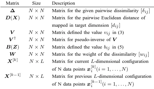
TABLE I
MAIN MATRICES USED INSMACOF
Matrix Size Description
∆ N×N Matrix for the given pairwise dissimilarity[δij]
D(X) N×N Matrix for the pairwise Euclidean distance of mapped in target dimension[dij]
V N×N Matrix defined the valuevijin (3)
V† N×N Matrix for pseudo-inverse ofV B(Z) N×N Matrix defined the valuebij in (5)
W N×N Matrix for the weight of the dissimilarity[wij]
X[k] N×L Matrix for currentL-dimensional configuration
of N data pointsx[ik](i= 1, . . . , N)
X[k−1] N×L Matrix for previousL-dimensional configuration of N data pointsx[ik−1](i= 1, . . . , N)
of a single process or even a single machine. Thus, running machine learning algorithms to process large dataset, including MDS and GTM discussed in this paper, in a distributed fashion is crucial so that we can utilize multiple processes and distributed resources to handle very large data which usually not fit in the memory of a single process or a compute node. The problem becomes more obvious if the running OS is 32-bit which can handle at most 4GB virtual memory per process. To process large data with efficiency, we have developed parallel version of MDS and GTM by using Message Passing Interface (MPI) fashion. In the following we will discuss more details how we decompose the MDS and GTM algorithm to fit in a memory limit in a single process or machine and implemented them by using MPI primitives.
A. Parallel SMACOF
Table I describes frequently used matrices in SMACOF algorithm, and memory requirement of SMACOF algorithm
increases quadratically as N increases. For the small dataset,
memory would not be any problem. However, it turns out to be critical problem when we deal with large data set, such
as thousands or even millions. For instance, if N = 10,000,
then one N ×N matrix of 8-byte double-precision numbers
consumes 800 MB of main memory, and if N = 100,000,
then one N ×N matrix uses 80 GB of main memory. To
make matters worse, SMACOF algorithm generally needs six
N×N matrices, so at least 480 GB of memory is required to
run SMACOF with 100,000 data points without considering
two N×Lconfiguration matrices in Table I.
If the weight is uniform (wij = 1,∀i, j), we can use only
four constants for representing N ×N V and V† matrices
in order to saving memory space. We, however, still need at
least threeN×N matrices, i.e.D(X),∆, andB(X), which
requires 240 GB memory for the above case, which is still infeasible amount of memory for a typical computer. That is why we have to implement parallel version of SMACOF with MPI.
To parallelize SMACOF, it is essential to ensure load bal-anced data decomposition as much as possible. Load balance is important not only for memory distribution but also for
M
00
M
01
M
02
[image:4.612.50.296.81.224.2]M
10
M
11
M
12
Fig. 1. N×Nmatrix decomposition of parallel SMACOF with 6 processes and 2×3 block decomposition. Dashed line represents where diagonal elements are.
computation distribution, since parallelization makes implicit benefit to computation as well as memory distribution, due to less computing per process. One simple approach of data
de-composition is that we assumep=n2, wherepis the number
of processes and n is an integer. Though it is relatively less
complicated decomposition than others, one major problem of this approach is that it is a quite strict constraint to utilize available computing processors (or cores). In order to release
that constraint, we decompose an N×N matrix to m×n
block decomposition, where m is the number of block rows
andnis the number of block columns, and the only constraint
of the decomposition is m×n = p, where 1 ≤ m, n ≤ p.
Thus, each process requires only approximately 1/p of full
memory requirements of SMACOF algorithm. Fig. 1 illustrates
how we decompose each N ×N matrices with 6 processes
and m = 2, n = 3. Without loss of generality, we assume
N%m=N%n= 0 in Fig. 1.
A process Pk,0 ≤k < p (sometimes, we will use Pij for
matchingMij) is assigned to one rectangular blockMij with
respect to simple block assignment equation in (16):
k=i×n+j (16)
where 0 ≤ i < m,0 ≤ j < n. For N ×N matrices, such
as ∆,V†,B(X[k]), and so on, each block Mij is assigned
to the corresponding process Pij, and for X[k]
andX[k
−1]
matrices,N×Lmatrices, each process has fullN×Lmatrices
because these matrices are relatively much small size and it results in reducing a number of additional message passing. By scattering decomposed blocks to distributed memory, now we are able to run SMACOF with huge data set as much as distributed memory allows in the cost of message passing overheads and complicated implementation.
At the iteration k in Alg. 1, the application should be
possible to acquire following information to do Line 8 and
Line 9 in Alg. 1: ∆, V†, B(X[k−1]), X[k−1], and σ[k].
One good feature of SMACOF algorithm is that some of
matrices are invariable, i.e.∆ andV†, through the iteration.
On the other hand, B(X[k−1]) and STRESS (σ[k]) value
x
=
M
M
00M
01M
02M
10M
11M
12X0
X1
X2
C0
C1
[image:5.612.312.564.39.547.2] [image:5.612.88.260.55.173.2]C
X
Fig. 2. Parallel matrix multiplication ofN×Nmatrix andN×Lmatrix based on the decomposition of Fig. 1
iteration. In addition, in order to update B(X[k−1]) and
STRESS (σ[k]) value in each iteration, we have to takeN×N
matrices information into account, so related processes should communicate via MPI primitives to obtain necessary infor-mation. Therefore, it is necessary to design message passing
schemes to do parallelization for calculating B(X[k−1])and
STRESS (σ[k]) value as well as parallel matrix multiplication
in Line 8 in Alg. 1.
Computing STRESS in (1) can be implemented simply
throughMPI_Allreduce. On the other hand, calculation of
B(X[k−1]) and parallel matrix multiplication is not simple,
specially for the case of m6=n. Fig. 2 depicts how parallel
matrix multiplication applies between an N ×N matrix M
and an N ×L matrix X. Parallel matrix multiplication for
SMACOF algorithm is implemented in three-step of message communication via MPI primitives. Block matrix
multiplica-tion of Fig. 2 for acquiring Ci (i = 0,1) can be written as
follows:
Ci= X
0≤j<3
Mij·Xj (17)
Since Mij of N ×N matrix is accessed only by the
corre-sponding processPij, computingMij·Xjpart is done byPij,
and the each computed sub-matrix, which is N2 ×Lmatrix for
Fig. 2, is sent to the process assignedMi0 by MPI primitives,
such as MPI_Send and MPI_Receive. Then the process
assignedMi0, sayPi0, sums the received sub-matrices to
gen-erateCi, and sendCiblock toP00. Finally,P00combines
sub-matrix blockCi 0≤i < mto constructN×LmatrixC, and
broadcast it to all other processes byMPI_Broadcast. Each
arrows in Fig. 2 represents message passing direction. Thin
dashed arrow lines describes message passing of N2 ×L
sub-matrices by MPI_Send and MPI_Receive, and message
passing of matrixC byMPI_Broadcastis represented by
thick dashed arrow lines. The pseudo code for parallel matrix multiplication in SMACOF algorithm is in Alg. 2
For the purpose of parallel computing B(X[k−1]), whose
elements bij is defined in (6), message passing mechanism
in Fig. 3 should be applied under 2 ×3 block
decompo-sition as in Fig. 1. Since bss = −P
s6=jbsj, a process
Pij, which is assigned toBij, should communicate a vector
sij, whose element is the sum of corresponding rows, with
Algorithm 2 Pseudo-code for distributed parallel matrix
mul-tiplication in SMACOF algorithm
Input: Mij,X
1: /*m=Row Blocks,n=Column Blocks*/
2: /*i=Rank-In-Row,j=Rank-In-Column*/
3: Tij =Mij·Xj
4: if j6= 0 then
5: SendTij toPi0 6: else
7: forj= 1 ton−1 do
8: ReceiveTij fromPij
9: end for
10: Generate Ci
11: end if
12: if i== 0andj== 0then
13: fori= 1tom−1 do
14: ReceiveCi from Pi0
15: end for
16: CombineC withCi wherei= 0, . . . , m−1
17: BroadcastC to all processes
18: else ifj== 0 then
19: SendCi toP00
20: Receive BroadcastedC
21: else
22: Receive BroadcastedC
23: end if
B
00
B
01
B
02
B
11
B
12
B
10
Fig. 3. Calculation ofB(X[k−1])matrix with regard to the decomposition
of Fig. 1.
processes assigned sub-matrix of the same block-row Pik,
wherek= 0, . . . , n−1, unless the number of column blocks
is 1 (n== 1). In Fig. 3, the diagonal dashed line indicates the
diagonal elements, and the green colored blocks are diagonal blocks for each block-row. Note that the definition of diagonal
blocks is a block which contains at least one diagonal element
of the matrix B(X[k]). Also, dashed arrow lines illustrate
message passing direction. Alg. 3 shows the pseudo-code of
Algorithm 3 Pseudo-code for calculating assigned sub-matrix
Bij defined in (6) for distributed-memory decomposition in
SMACOF algorithm
Input: Mij,X
1: /*m=Row Blocks,n=Column Blocks*/
2: /*i=Rank-In-Row,j =Rank-In-Column*/
3: /* We assume that subblock Bij is assigned to process
Pij */
4: Find diagonal blocks in the same row (rowi)
5: if Bij ∈/ diagonal blocks then
6: compute elementsbst ofBij
7: Send a vectorsij, whose element is the sum of
corre-sponding rows, toPik, whereBik ∈diagonal blocks
8: else
9: compute elementsbst ofBij, wheres6=t
10: Receive a vector sik, whose element is the sum of
corresponding rows, where k = 1, . . . , n from other
processes in the same block-row
11: Send sij to other processes in the same block-row∈
diagonal blocks
12: Computebss elements based on the row sums.
13: end if
TABLE II
MAIN MATRICES USED INGTMFORNDATA POINTS IND-DIMENSION
WITHKLATENT POINTS INL-DIMENSION.
Matrix Size Description
Z K×L Matrix for K latent pointszk(k= 1, ..., K)
Φ K×M Design matrix with M-dimension
W M×D Matrix for parameters
Y K×D Matrix for K mapped pointsyk(k= 1, ..., K)
X N×D Matrix for N data pointsxn(n= 1, ..., N)
R K×N Matrix for K responsibilities for each N data points
B. Parallel GTM
Among many matrices allocated in memory for processing in GTM as summarized in Table II, the responsibility matrix
R is the most biggest one. For example, the matrix R for
8,000 latent points, corresponding to 20x20x20 3D grid, with 100,000 data points needs at least 6.4GB memory space saving 8-byte double precision numbers and even without considering additional memory requirements for other matrices, this easily prevents us from processing large data set in GTM by using a single process or machine. Thus, we have focused on
the decomposition of responsibility matrix R in developing
parallel GTM.
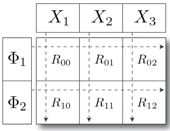
As shown in Fig. 4, in our parallel GTM we decompose
the design matrix Φ ∈RK×M into m row-based sub-blocks
denoted by {Φi}m−i=01 so that each sub-blockΦi has
approxi-matelyK/mrows ofΦ. In the same way, we also decompose
the data matrix X into n row-based sub-blocks {Xj}n−j=01,
each of which having approximatelyN/n rows ofX. Then,
we can compute the sub-matrix Rij (i = 0, ..., m−1, j =
0, ..., n−1)for the latent pointsYi=ΦiW (Yiis alsoi-th
R
00R
10R
01R
02R
12R
11Φ
1
Φ
2
[image:6.612.345.519.51.185.2]X
1
X
2
X
3
Fig. 4. Data decomposition of parallel GTM for computing responsibility matrixRby using 2-by-3 mesh of computing nodes.
row-based sub-block ofY) and data pointsXjon them-by-n
mesh of logical compute grid where(i, j)-th node computes
Rij which consumes only 1/mn of memory space for the
full matrix R. Without loss of generality, we assume that
K%m=N%n= 0 and denoteK¯ =K/mandN¯ =N/n.
Since our parallel GTM algorithm is not a pleasingly parallel application in which no dependency is needed between compute nodes but rather a typical parallel problem which can be solved by using a general map-reduce approach. To have systematic communication model, we can use MPI’s
cartesian grid topology in our m-by-n compute grid so that
each node belongs to both row communications and column
communications, denoted by ROW-COMM and COL-COMM
respectively hereafter.
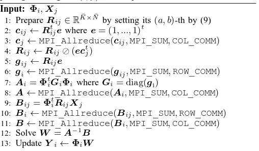
More details of our parallel GTM algorithm is as follows.
1) Initialization Prepare subblock data {Φi}m−i=01 and
{Xj}n−j=01 and distribute them to i-th row members
and j-th column members respectively in the m-by-n
compute grid.
2) Responsibility Initialize the responsibility matrix Rij
by setting(a, b)-th elementrab=N(xb|ya), as defined
in (9), fora= 0, ...,K−¯ 1andb= 0, ...,N¯−1. Compute
the column sumcij ∈RN¯ ofRij and exchange it with
row members to get ci =Pn−1
j=0cij and compute
Rij =Rij⊘(ectj) (18)
whereeis a vector of(1, ...,1)t∈RK¯ and⊘represents
element-wise division.
3) Optimization Compute a row-sum vector gij = Rije
and exchange it with row members to get gi =
Pn−1
j=0 gij. Compute a matrix Ai = ΦtiGiΦi where
Gi is a diagonal matrix whose diagonal elements are
gi and exchange with column members to compute
A = Pm−1
i=0 Ai. Prepare another matrix Bij =
ΦtiRijXj and exchange it with row-members to get
Bi=Pn−1
j=0 Bij, followed by exchanging with column
members to compute B = Pm−1
i=0 Bi. Finally, solve
AW =Bwith respect to the parameter matrixW and
Algorithm 4 Pseudo-code for distributed parallel GTM
com-puting running on (i, j)-th compute node.
Input: Φi,Xj
1: PrepareRij∈R
¯
K×N¯
by setting its(a, b)-th by (9)
2: cij←Rtijewheree= (1, ...,1) t
3: cj←MPI_Allreduce(cij,MPI_SUM,COL_COMM)
4: Rij←Rij⊘(ectj)
5: gij←Rije
6: gi←MPI_Allreduce(gij,MPI_SUM,ROW_COMM)
7: Ai=ΦtiGiΦi whereGi= diag(gi)
8: A←MPI_Allreduce(Ai,MPI_SUM,COL_COMM)
9: Bij=ΦtiRijXj
10: Bi←MPI_Allreduce(Bij,MPI_SUM,ROW_COMM)
11: B←MPI_Allreduce(Bi,MPI_SUM,COL_COMM)
12: SolveW =A−1B
13: UpdateYi←ΦiW
continue to run until we find the parameter matrixW
converged.
Exchanging data with row (or column) members of the grid and collecting them, we can use a MPI primitive function
MPI_Allreduce with MPI_SUM collective opeartion. A
pseudo code with MPI functions is shown in Alg. 4.
IV. PERFORMANCE ANDCORRELATIONMEASUREMENT
For the performance analysis of both parallel SMACOF and parallel GTM discussed in this paper, we have applied our par-allel algorithms for high-dimensional data visualization in
low-dimension to the dataset obtained from PubChem database1,
which is a NIH-funded repository for over 60 million chemical molecules and provides their chemical structure fingerprints and biological activities, for the purpose of chemical infor-mation mining and exploration. Among 60 Million PubChem dataset, in this paper we have used randomly selected up to 100,000 chemical subsets and all of them have a 166-long binary value as a fingerprint, which corresponds to maximum input of 100,000 data points having 166 dimensions. With those data as inputs, we have performed our experiments on our two decent compute clusters as summarized in Table III.
In the following, we will show the performance results of our parallel SMACOF and GTM implementation with respect to 10,000, 20,000, 50,000 and 100,000 data points having 166 dimensions, represented as 10K, 20K, 50K, and 100K dataset respectively and discuss the correlation measurement between SMACOF and GTM results by using CCA.
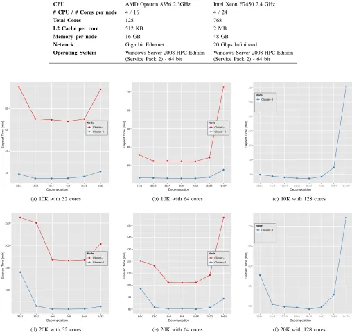
[image:7.612.49.303.77.225.2]A. Performance of Parallel SMACOF
Fig. 5 shows the performance comparisons for 10K and 20K PubChem data with respect to how to decompose the given
N ×N matrices with 32, 64, and 128 cores in Cluster-I and
Cluster-II. A significant characteristic of those plots in Fig. 5
is that skewed data decompositions, such as p×1 or1×p,
which decompose by row-base or column-base, are always worse in performance than balanced data decompositions, such
as m×nblock decomposition whichmandnare similar as
1PubChem,http://pubchem.ncbi.nlm.nih.gov/
much as possible. The reason of the above results is cache line effect that affects cache reusability, and generally balanced block decomposition shows better cache reusability so that it occurs less cache misses than the skewed decompositions [20], [21]. As in Fig. 5, Difference of data decomposition almost
doubled the elapsed time of1×128decomposition compared
to 8 × 16 decomposition with 10K PubChem data. From
the above investigation, the balanced data decomposition is generally good choice. Furthermore, Cluster-II performs better than Cluster-I in Fig. 5, although the clock speed of cores is similar to each other. There are two different factors between Cluster-I and Cluster-II in Table III which we believe that those factors result in Cluster-II outperforms than Cluster-I, i.e. L2 cache size and Networks, and the L2 cache size per core is 4 times bigger in Cluster-II than Cluster-I. Since SMACOF with large data is memory-bound application, it is natural that the bigger cache size results in the faster running time.
In addition to data decomposition experiments, we mea-sured the parallel performance of parallel SMACOF in terms
of the number of processes p. The authors investigate the
scalability of parallel SMACOF by running with different
number of processes, e.g. p = 64, 128, 256, and 384. On
the basis of the above data decomposition experimental result, the balanced decomposition has been applied to this process
scaling experiments. Asp increases, the elapsed time should
be decreased, but linear performance improvement could not be achieved due to the parallel overhead. In Fig. 6, both 50k
and 100k data sets show the performance gain aspincreases.
However, performance enhancement ratio is reduced, because the ratio of message passing overhead over the assigned computation per each node increases due to more messaging
and less computing per node as p increases. Note that we
used 16 computing nodes in Cluster-II (total number of cores in 16 computing nodes is 384 cores) to perform the scaling experiment with large data set, i.e. 50k and 100k PubChem data, since SMACOF algorithm requires 480 GB memory for dealing with 100,000 data points, as we disscussed in Section III-A, and Cluster-II is only feasible to perform that with more than 10 nodes.
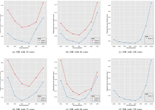
B. Performance of Parallel GTM
We have measured performance of parallel GTM with
re-spect to each possiblem-by-ndecomposition of responsibility
matrix R to use p = 32, 64, and 128 cores in
Cluster-I and Cluster-Cluster-ICluster-I for 10k and 20k PubChem dataset. Cluster-In the following experiments, we have fixed other parameters such
as K= 8,000,D= 166, and M = 9.
As shown in Fig. 7, the performance of parallel GTM shows the similar pattern of the parallel SMACOF performance in which the balanced decomposition performs better than the skewed decomposition due to the cache line effect.
C. Correlation measurement by CCA
TABLE III
CLUSTER SYSTEMS USED FOR THE PERFORMANCE ANALYSIS
Features Cluster-I Cluster-II # Nodes 8 32
CPU AMD Opteron 8356 2.3GHz Intel Xeon E7450 2.4 GHz
# CPU / # Cores per node 4 / 16 4 / 24
Total Cores 128 768
L2 Cache per core 512 KB 2 MB
Memory per node 16 GB 48 GB
Network Giga bit Ethernet 20 Gbps Infiniband
Operating System Windows Server 2008 HPC Edition (Service Pack 2) - 64 bit
Windows Server 2008 HPC Edition (Service Pack 2) - 64 bit
Decomposition
Elapsed Time (min)
40 45 50 55
32x1 16x2 8x4 4x8 2x16 1x32
Node
Cluster−I Cluster−II
(a) 10K with 32 cores
Decomposition
Elapsed Time (min)
30 40 50 60 70
64x1 32x2 16x4 8x8 4x16 2x32 1x64
Node
Cluster−I Cluster−II
(b) 10K with 64 cores
Decomposition
Elapsed Time (min)
16 18 20 22 24 26 28
128x1 64x2 32x4 16x8 8x16 4x32 2x64 1x128
Node
Cluster−II
(c) 10K with 128 cores
Decomposition
Elapsed Time (min)
160 180 200 220
32x1 16x2 8x4 4x8 2x16 1x32
Node
Cluster−I Cluster−II
(d) 20K with 32 cores
Decomposition
Elapsed Time (min)
80 90 100 110 120 130 140 150
64x1 32x2 16x4 8x8 4x16 2x32 1x64
Node
Cluster−I Cluster−II
(e) 20K with 64 cores
Decomposition
Elapsed Time (min)
50 55 60 65 70
128x1 64x2 32x4 16x8 8x16 4x32 2x64 1x128
Node
Cluster−II
[image:8.612.56.564.104.583.2](f) 20K with 128 cores
Fig. 5. Performance of Parallel SMACOF for 10K and 20K PubChem data with 32,64, and 128 cores in Cluster-I and Cluster-II w.r.t. data decomposition ofN×N matrices.
of both results is about 0.90 which is close to the maximum (1.0) and so we can conclude that both MDS and GTM algorithms produces very similar output for the 100k dataset. Also, we have used the colors in Fig. 8 to identify two
clusters as an output of k-mean (k = 2) clustering in the
original 166-dimensional space. The output shows both MDS and GTM successfully preserved the cluster information in low dimension.
V. CONCLUSIONS ANDFUTUREWORKS
number of processes
Elapsed Time (min)
27.5 28 28.5 29 29.5 210 210.5
26 26.5
27 27.5
28 28.5
Size
[image:9.612.90.260.59.230.2]100k 50k
Fig. 6. Performance of parallel SMACOF for 50K and 100K PubChem data in Cluster-II w.r.t. the number of processes. Based on the data decomposition experiment, we choose balanced decomposition as much as possible, i.e.8×8
for 64 processes. Note that both x and y axes are log-scaled.
run SMACOF algorithm with 100,000 data points. Paralleliza-tion via tradiParalleliza-tional MPI approach in order to utilize distributed memory computing system, which can extend the accessible memory size, is proposed as a solution for the amendment of memory shortage to treat large data with SMACOF and GTM algorithms.
As we discussed in the performance analysis, the data decomposition structure is important to maximize the per-formance of parallelized algorithm since it highly affects to message passing routines and message passing overhead as
well as cache-line effect. Balanced data decomposition (m×n)
is generally better than skewed decomposition (p×1or1×p)
for both algorithms, specially for the MDS algorithm. Another interesting aspect we found here is that the MDS and GTM results of the same data are highly correlated with each other as in Fig. 8 (c) even though the detailed mappings to low dimension are visually distinct as shown in Fig. 8(a) and (b).
There are important problems for which the data set size is too large for even our parallel algorithms to be practical. Because of this, we are now developing interpolation ap-proaches for both algorithms. Here we run MDS or GTMs with a (random) subset of the dataset, and the dimension reduction of the remaining points are interpolated. We will report on this extension in a later paper where we will test on the full 60 million PubChem dataset. We will also present results elsewhere on cases such as gene sequences where only dissimilarities and not vectors are involved. We will compare different choices (as suggested by Sammon’s algorithm [22])
for the weight function wij in (1) and (2).
ACKNOWLEDGEMENT
We would like to thank to Professor David Wild and Dr. Qian Zhu in the School of Informatics and Computing, Indiana University, for their valuable advices and feedbacks
on PubChem data and analysis. We would also like to thank Microsoft for their collaboration and support.
REFERENCES
[1] G. Fox, S. Bae, J. Ekanayake, X. Qiu, and H. Yuan, “Parallel data mining from multicore to cloudy grids,” in Proceedings of HPC 2008 High Performance Computing and Grids workshop, Cetraro, Italy, July 2008.
[2] C. Bishop, M. Svens´en, and C. Williams, “GTM: A principled alternative to the self-organizing map,” Advances in neural information processing systems, pp. 354–360, 1997.
[3] ——, “GTM: The generative topographic mapping,” Neural computa-tion, vol. 10, no. 1, pp. 215–234, 1998.
[4] T. Kohonen, “The self-organizing map,” Neurocomputing, vol. 21, no. 1-3, pp. 1–6, 1998.
[5] J. B. Kruskal and M. Wish, Multidimensional Scaling. Beverly Hills, CA, U.S.A.: Sage Publications Inc., 1978.
[6] I. Borg and P. J. Groenen, Modern Multidimensional Scaling: Theory and Applications. New York, NY, U.S.A.: Springer, 2005.
[7] J. B. Kruskal, “Multidimensional scaling by optimizing goodness of fit to a nonmetric hypothesis,” Psychometrika, vol. 29, no. 1, pp. 1–27, 1964.
[8] Y. Takane, F. W. Young, and J. de Leeuw, “Nonmetric individual differences multidimensional scaling: an alternating least squares method with optimal scaling features,” Psychometrika, vol. 42, no. 1, pp. 7–67, 1977.
[9] J. de Leeuw, “Applications of convex analysis to multidimensional scaling,” Recent Developments in Statistics, pp. 133–145, 1977. [10] ——, “Convergence of the majorization method for multidimensional
scaling,” Journal of Classification, vol. 5, no. 2, pp. 163–180, 1988. [11] A. Dempster, N. Laird, and D. Rubin, “Maximum likelihood from
incomplete data via the em algorithm,” Journal of the Royal Statistical Society. Series B, pp. 1–38, 1977.
[12] E. H. Moore, “On the reciprocal of the general algebraic matrix,” Bulletin of American Mathematical Society, vol. 26, pp. 394–395, 1920. [13] R. Penrose, “A generalized inverse for matrices,” Proceedings of the
Cambridge Philosophical Society, vol. 51, pp. 406–413, 1955. [14] H. Hotelling, “Relations between two sets of variates,” Biometrika,
vol. 28, no. 3, pp. 321–377, 1936.
[15] D. Hardoon, S. Szedmak, and J. Shawe-Taylor, “Canonical correlation analysis: an overview with application to learning methods,” Neural Computation, vol. 16, no. 12, pp. 2639–2664, 2004.
[16] H. Glahn, “Canonical correlation and its relationship to discriminant analysis and multiple regression,” Journal of the Atmospheric Sciences, vol. 25, no. 1, pp. 23–31, 1968.
[17] O. Friman, J. Cedefamn, P. Lundberg, M. Borga, and H. Knutsson, “De-tection of neural activity in functional MRI using canonical correlation analysis,” Magnetic Resonance in Medicine, vol. 45, no. 2, pp. 323–330, 2001.
[18] N. Campbell and W. Atchley, “The geometry of canonical variate analysis,” Systematic Zoology, pp. 268–280, 1981.
[19] B. Thompson, Canonical correlation analysis uses and interpretation. Sage, 1984.
[20] X. Qiu, G. C. Fox, H. Yuan, S.-H. Bae, G. Chrysanthakopoulos, and H. F. Nielsen, “Data mining on multicore clusters,” in Proceedings of 7th International Conference on Grid and Cooperative Computing GCC2008. Shenzhen, China: IEEE Computer Society, Oct. 2008, pp. 41–49.
[21] S.-H. Bae, “Parallel multidimensional scaling performance on multicore systems,” in Proceedings of the Advances in High-Performance E-Science Middleware and Applications workshop (AHEMA) of Fourth IEEE International Conference on eScience. Indianapolis, Indiana: IEEE Computer Society, Dec. 2008, pp. 695–702.
Decomposition
Elapsed time per iter
ation (sec)
0.08 0.10 0.12 0.14
32x1 16x2 8x4 4x8 2x16 1x32
Node
Cluster−I Cluster−II
(a) 10K with 32 cores
Decomposition
Elapsed time per iter
ation (sec)
0.06 0.08 0.10 0.12 0.14
64x1 32x2 16x4 8x8 4x16 2x32 1x64
Node
Cluster−I Cluster−II
(b) 10K with 64 cores
Decomposition
Elapsed time per iter
ation (sec)
0.05 0.10 0.15 0.20 0.25 0.30 0.35
128x1 64x2 32x4 16x8 8x16 4x32 2x64 1x128
Node
Cluster−II
(c) 10K with 128 cores
Decomposition
Elapsed time per iter
ation (sec)
0.14 0.16 0.18 0.20 0.22
32x1 16x2 8x4 4x8 2x16 1x32
Node
Cluster−I Cluster−II
(d) 20K with 32 cores
Decomposition
Elapsed time per iter
ation (sec)
0.10 0.12 0.14 0.16 0.18 0.20 0.22
64x1 32x2 16x4 8x8 4x16 2x32 1x64
Node
Cluster−I Cluster−II
(e) 20K with 64 cores
Decomposition
Elapsed time per iter
ation (sec)
0.10 0.15 0.20 0.25 0.30 0.35 0.40
128x1 64x2 32x4 16x8 8x16 4x32 2x64 1x128
Node
Cluster−II
[image:10.612.60.568.67.428.2](f) 20K with 128 cores
Fig. 7. Performance of Parallel GTM for 10K and 20K PubChem data with 32, 64, and 128 cores running on Cluster-I and Cluster-II w.r.t. them-by-ndata decomposition running on compute grids. The elapsed time is an average running time per iteration.
(a) MDS for 100K PubChem (b) GTM for 100K PubChem
1st Canonical Variable for GTM
1st Canonical V
ar
iab
le f
or MDS
−2e−05 −1e−05 0e+00 1e−05 2e−05
−2e−05 −1e−05 0e+00 1e−05
(c) Canonical variables plot for MDS and GTM
[image:10.612.65.550.482.667.2]