Theses Thesis/Dissertation Collections
1990
Statistical mechanics of neural networks and
combinatorial optimization problems
David L. Morabito
Follow this and additional works at:http://scholarworks.rit.edu/theses
This Thesis is brought to you for free and open access by the Thesis/Dissertation Collections at RIT Scholar Works. It has been accepted for inclusion in Theses by an authorized administrator of RIT Scholar Works. For more information, please [email protected].
Recommended Citation
Rochester Institute of Technology
School of Computer Science and Information Technology
Statistical Mechanics Of Neural Networks
And
Combinatorial Optimization Problems
by
David
L.Morabito
A thesis, submitted to
The Faculty of the School of Computer Science and Information Technology in partial fulfillment of the requirements for the degree of
Master of Science in Computer Science. 1991
Approved by:
Professor Peter Anderson
Professor Stanislaw Radziszowski
Title of Thesis:
Statistical Mechanics of Neural Networks and Combinatorial Optimization Problems.
I prefer to be contacted
each time a request for reproduction is made. I can be reached at the following address:
David L. Morabito 9805 Union St.
Scottsville, N.Y. 14546
ACKNOWLEDGEMENTS
I want to thank my parents for all their love and support throughout my many years in
Local learning neural networks have long been limited by their inability to store correlated patterns. A common parameter used to specify the capacity of a network is
<X =piN, wherep is the number of stored patterns andN is the number of neurons in
the network. Using statistical mechanics I have found that a network using nonlocal learning rules has better retrieval qualities than a network using local learning rules. In particular, the analysis has determined that nonlocal learning rules give a maximum capacity of <Xc
=
1, which is a significant increase over local learning rules in whichthe maximum capacity is never greater than <Xc
=
0.14. Computer simulations for anonlocal learning network are also presented.
KEY WORDS AND PHRASES
Associative recall - Different input stimulus will lead to a similar output stimuli.
Asynchronous dynamics Neurons are picked in a random sequence for updating. Updating of each neuron is dependent on the previous network state.
Attractor - A state, or a restricted set of states, which is dynamically reached by a large collection of input states after a long enough time.
Attractor Neural Network (ANN) A non-linear network whose long time behavior is governed by attractors.
Basin of attraction - Set of states which are attracted to the same attractor.
Ergodicity - A system will sample all of its possible states in a finite amount of time.
Excitatory - A synaptic connection that increases the likelihood that a neuron will fire.
Fixed-point - A network state that is continually repeated in the course of the dynami-cal evolution of the network.
Free-energy - A quantity that is decreased as a system follows some dynamical pro-cess.
Frustration Contradictory requests are made on a neuron. This is brought about by having both inhibitory and excitatory connections to the same neuron.
Inhibitory - A synaptic connection that reduces the likelihood that a neuron will fire.
Network state Instantaneous state of all neurons that make up the network.
Overlap - Measures the nearness of twoN bit words.
Retrieval - Specification that a network has reached an attractor state. Will be signified by a special bursting of neurons.
Spurious state - Pattern that has not been stored by a network.
0.2.1 Combinatorics
TABLE OF CONTENTS
1 INTRODUCTION .
1.1. Motivation and Goals
1.1.1. Motivation
1.1.2. Goals
1.2. Neurophysiological Background .
1.3. Formal Neurons and Perceptrons .
1.4. Attractor Neural Networks (ANN) ..
1.4.1. ANN Assumptions .
1.5. Significant Network States .
1.6. Spontaneous Computation vs. Cognitive Processing .
2 SPIN GLASSES
2.1. Introduction
2.1.1. Simple Model .
2.1.1.1. Ground States .
2.1.1.2. Neuronal Language .
2.2. Random Ising Magnetic System .
2.3. Previous Work and Problem Specification ..
2.4. Theoretical and Conceptual Development .
3 ANN AND NONLOCAL LEARNING ..
3.2. Personnaz Model .
3.3. Noiseless Dynamics
3.4. Self-Coupling in Personnaz Model .
3.5. Non-local Learning Model with an Energy Function .
3.5.1. Connection with Hopfield Model .
3.5.2. Global Minima of E .
3.6. Simulations of Network ,
4 REPLICA METHOD AND GRAPH PARTITIONING .
4.1. General Information
4.2. Problem Specification .
4.3. Cost Function .
4.4. Free Energy Expression .
5 CONCLUSIONS .
5.1. State Of The Subject .
5.2. Future Work .
BIBLIOGRAPHY .
APPENDIX .
27 28 29
32 33 36 39
40
40
40
42
FIGURES
[image:10.553.73.492.154.285.2]Figure 1.1: XOR using Fonnal neurons 5
Figure 1.2: Multi-perceptron 6
Figure 1.3: Multi-perceptron used to fonn ANN 7
Figure 1.4: Dynamics of 5 neuron ANN 8
Figure 1.5: Geometrical representation of network states 10
Figure 1.6: Spontaneous computation 12
Figure 2.1: Frustrated spin system 17
INTRODUCTION
1.1. Motivation and Goals
1.1.1. Motivation
Biological neurons, though numerous in size, structure type and functionality, all
"fire" a signal (voltage potential) down their axon if the sum of the inputs at their
soma reaches the neurons "firing" potential. Since magnetic systems in nature exhibit
many of the features of neural systems, the tools and concepts used in studying
mag-netic systems should also be applicable to the study of neural networks. To a
neuro-biologist this may seem to be a useless endeavor. In Physics the major tool for
study-ing many-body problems (includstudy-ing an infinite number of bodies) is statistical
mechan-ics. If we were actually trying to model the dynamics of some system it would be necessary to consider the actual structure of the system. On the other hand, if we were
concerned with the long time behavior of a system it is not necessary to consider the
structure. Given the rules for the interaction of one piece of the system with another
piece of the system we can effectively compute the long time behavior of the system.
In other words the actual structure of the system, be it a biological neuron or a
mag-netic spin system, is hidden inside the interaction rule.
2
1.1.2. Goals
Hopfield, using this approach, analyzed a local learning neural network [Hopfield82]. The particular magnetic system used was an Ising spin glass [Pathria80, Huang62, Kubo65, Feynman62]. The Ising model for a spin glass is a very naive model. The first topic of this thesis is to model a neural network that uses nonlocal learning instead of local learning. The second topic of this thesis is to use statistical mechanics to solve the graph q-partitioning problem analytically.
1.2. Neurophysiological Background
The subject of neural networks can be approached from two different angles: the first is concerned with massive parallel computers. Usually this area is not concerned with questions of biological plausibility. Mainly, questions of computational speed and efficiency are addressed. The second category is a study of model networks that exhi-bit many of the characteristics of a biological neural system. There are six criteria that will be considered important in any theory of a neural network [Amit89]:
• Biological plausibility - simply the requirement that the elements composing the network not be outlandish from a physiological point of view.
• Associativity - impression that many similar inputs are basically collapsed on a prototype for purposes of cognition and manipulation - a picture viewed from any angle and in different light and shading represents a single individual.
whole reacts to tasks that are prohibitive to high-speed serial computers.
• Emergent behavior - stands for an input-output relation which is rather unlikely
(non-generic) given the system's elements.
• Freedom from homunculi - eternal goal of eliminating little external observers
which could assign meaning to outputs.
• Potential for abstraction - the ability of a network to operate similarly on a
variety of inputs that are not simply associated in form but are classified together
only for the purpose of the particular operation.
It is important that we know the stages that an individual neuron goes through to
determine if it will fire or not:
(1) A neuron either is in a state of dormancy or in a firing state. In the firing state an action potential is effectively propagated unchanged down the axon.
(2) When the action potential reaches the end of the axon, neuro-transmitters are
emitted in the post-synaptic cleft.
(3) When the neuro-transmitters reach the membrane of the post-synaptic neuron,
ionic current is allowed to enter the post-synaptic neuron. The amount of current
is a measure of the efficacy of the synapse.
(4) The ionic current generates a Post Synaptic Potential (PSP). (Note: Throughout
the rest of this thesis the PSP at a particular neuron, labelled by i, will be
represented by hi). This potential is gradually reduced as the PSP travels toward
the soma. A PSP can be either excitatory (Le. increasing the probability of the
4
(5) A neuron will fire (i.e. transmit an action potential - indicated below by 0'= 1) if
the sum, calculated at the soma, of all incoming PSP's is greater than the
neuron's threshold potential. If the sum of PSP's is less than the threshold, the
neuron is dormant (i.e. it does not transmit an action potential - indicated below
by 0' = 0).
1.3. Formal Neurons and Perceptrons
We can formally specify the condition for the neuron to fire in the manner
prescribed in the Section 1.2:
N
hi =
L
Iij O'j (1.1)j=l
where the Iij's are called the synaptic efficacies. The output of neuron i depends on
the value of hi in comparison with the threshold potential at neuron i (Ti ).
Symboli-cally, we can represent the spiking condition as:
ifhi >Ti
otherwise
(1.2)
Thus
0';
=
1 indicates that the neuron will spike (fire an action potential) while0';
=
0indicates that the neuron is dormant. Using that fact that 0 and 1 can be used to
represent the values true and false, McCulloch and Pitts [Pitts43] proposed that a
co1-lection of neurons could be connected into a temporal sequence at the end of which
there would be a single output neuron whose output would be the value of the logical
expression imprinted on the network at the beginning of the temporal sequence. Refer
to Figure 1.1 for the construction of the exclusive or of A and B by a collection of
t t +1 t +2 t+3
T=-l.
2
A (-1 )
'~T-J
lAND) I~EG) ~ (A, B)
?
(1) 2 (AND)
B ...
[image:15.553.92.442.78.224.2](OR) (IDENTITY)
Figure 1.1: The construction for the exclusive or (xor bythe route [A +B H...,[A·B]] [Amit89].
Realizing that any true neuron will have approximately 104 input synaptic con-nections, Rosenblatt [Rosenblatt62] proposed that a fonnal neuron can have any number of inputs. There is still only one output neuron but we now have any number of inputs into that output neuron. A perceptron is a linear threshold device (i.e. no feedback of any type is present in the network) just as a fonnal neuron is. The best that can be accomplished is a two-fold classification of input values. A network that has N input values can accommodate 2N different input patterns (i.e. patterns of 1's and O's). Since the output neuron can generate either a 1 or a 0 we can classify the input into two classes. One class represents all input that generates a 1 output while the other represents all input that generates a 0 output.
'""
6
j = 1
j =2
j =3
j=N
• • •
i=2
~~~~
• [image:16.555.108.381.48.265.2]• •
Figure 1.2: A single layer multi-perceptron [Amit89].
the input patterns into classes depending on the output pattern that they produce. The number of classes and the actual pattern each class corresponds to is determined by the value for the synaptic efficacies.
1.4. Attractor Neural Networks (ANN)
If we close a multi-perceptron upon itself we have a network where the output axons are identified also as input axons - this is a closed system that is not an input-output system (see Figure 1.3). In such a system once a network state is repeated once, it will be repeated indefinitely. These states are called the "attractors" of the dynamics. The idea behind the concept of an attractor is that when a network is prepared in a state close to an attractor state it will, through the dynamics of the net-work, progress to the attractor state (i.e. the initial state is attracted to the attractor state). The following notation will be used. Tj is the threshold of the jth neuron and
representa-Figure 1.3: A multi-perceptron closed on itselftofonn an ANN [Amit89].
tion for OJ as:
",('+1) = {
~
ifhj(t+l) - Tj >0otherwise
(1.3)
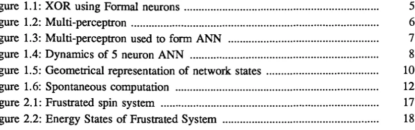
In other words this means that if OJ is 1 the neuron is firing, while ifOJ is 0 the neu-ron is donnant. For a graphical example of a 5 neuneu-ron network see Figure 1-4.
1.4.1. ANN Assumptions
ANN's have the following assumptions that have immediate neurobiological meaning.
• The individual neurons have no memory.
This is manifest in the fact that no thresholds vary in time (i.e. no modification due to past happenings).
[image:17.552.104.317.49.259.2]8
Time
J,; t
; - 1 2 3 4 5 2 3 4 5
1 0;
•
0
• • •
0 0 -0.6 0 -0.2h; (-0.8) (-0.8)(-0.4)(-0.2)(-0.2)
2 0;
0 0 0
• •
2 0.6 0 -0.6 0 -0.2T= -0.3
h; (-0.2) (0.4) (-1.6) (0.4) (-0.6) 3 -0.6 -0.6 0 -0.6 0.2
3 0;
•
•
0
•
0
4 0 0.6 -0.6 0 -0.2h; (0.0) (0.6) (-1.8) (0.6) (-0.6) 4
• •
0
•
0
5 -0.2 -0.2 0 -0.2 00;
;
-Figure 1.4: Dynamics of a five neuron network with thresholds Tj =-0.3 and a connection matrixJi ·.
White neurons are resting, black ones have spiking axons. Note that following t = 3all states will ~ identical. This is an example of a fixed-point attractor [Amit89].
In physics when there are competing tendencies throughout the system we say that the system is frustrated. Frustration is the underlying reason why a network will have many energy minima each of which corresponds to a stored pattern. The whole idea behind frustration will be treated in much more depth at a later time.
• The synaptic connections are all symmetric.
This is fonnally written as Jij = Jji . This is an indispensable tool in the study of ANN's but it has no biological foundation. This would be worrisome to biolo-gists, but it has been formally shown [Amit89] that when the symmetry restraint is lifted no major modifications are seen in the behavior of the network.
[image:18.552.85.435.93.263.2]This is a reasonable assumption to make since in a true neural system there does
not seem to be any notion of a master clock indicating when each neuron in the
network should update. Each neuron chooses to fire or not to fire within a preset time frame (after this time the PSP at the soma gradually is degraded). Also,
when physical separations are included in the analysis it is apparent that updates
of nearby neurons will only effect the neuron that is choosing to fire if those
nearby neurons are within a certain length.
1.5. Significant Network States
A network state is defined to be the collection of the individual states (i.e. is the
neuron firing or dormant) of each neuron. Thus a network state is made up of N
numbers where each number can be 0 (dormant) or 1 (firing). In an ANN not all
net-work states are significant. Shortly, we will see that only fixed-point sequences will
have any dynamical significance. Before discussing fixed-points we must develop
some terminology. Consider the fact that the state of a network of N neurons is
specified by giving N values each of which can be only 0 or 1. Geometrically, these
values can be viewed as labelling the vertices of an N-dimensional hypercube (see
Figure 1.5). In this light a fixed-point can be defined as the sequence in which all net-work states remain at the same vertex in the hypercube (Note: The collection of
ver-tices of the hypercube is sometimes called the space of network states.). All of this is
important but we are striving for a way to represent the following three concepts:
10
2
(-11 -1) (11-1)
(-111 )f"---:....~r:(111)
[image:20.552.101.340.55.275.2]3
Figure 1.5: Geometrical representation of the distance betweenpairs of network states [Amit89].
• generation of meaning
• self-recognizability, i.e., freedom from homunculus
Even though the network state is unchanged, it does not mean that the neurons are dormant. On the contrary, when a network is in a fixed point, the average firing rate for a neuron is at its maximum. This fact alone allows for self-recognizability through the calculation of the mean neural firing rate. Thus, fixed points will be identified with cognitive events.
1.6. Spontaneous Computation vs. Cognitive Processing
model - [Willshaw69]), and Kohonen and Palm (error reducing projections
-[Kohonen84]). Feed-forward networks are further categorized as input systems since
for each network input state there is an output state that can only be categorized as
good or bad after looking at its content. In these cases we say that spontaneous
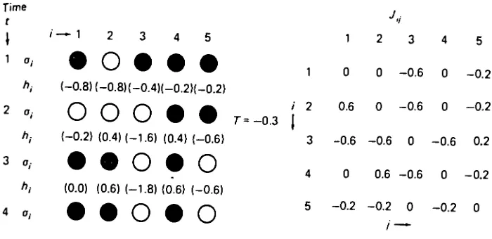
com-putation has taken place (see Figure 1.6). Hence, in such networks the notion of a
fixed point is meaningless. In actuality, all network states would correspond to a
cog-nitive event. Thus, in many feed-forward networks the notion of an internal
homun-culus cannot be discarded.
In contrast, Little [Little74] and especially Hopfie1d [Hopfield82] have introduced
the notion of Attractor Neural Networks. The major difference between feed-forward
and dynamical attractor networks is that in an ANN there is not necessarily a
meaning-ful output state for each input state. As discussed earlier the output states are
mean-ingful when the network is in an attractor state of which a fixed point is only the
sim-plest version.
The major study concerning ANN's deals with their use as associative memories.
Acting as an associative network the attractor states will correspond with the stored
memories "learned" by the network. Using the same idea, we can tum an ANN into a
computational network. What is required for an ANN to be used for a computation is
that the result of the computation corresponds to an attractor of the network. Thus, the
notion of temporary results is not necessary or tenable. The following common
12
(1) Traveling salesman (2) Matching problem
(3) Graph partitioning problem o
[image:22.552.61.467.64.564.2]o
Figure 1.6: A network which spontaneously computes the sum of two 8-bit words, the top and the bot-tom input units (open circles on left) and represents the sum on the 8 output units (full squares on
right). The internal elements are logical gates with two inputs and several outputs. The full
SPIN GLASSES
2.1. Introduction
Before discussing spin glasses it may be instructive to discuss some of the basic
similarities between random magnetic systems and neural networks [Gutfreund85].
Any magnetic system can be naively viewed as a collection of magnetic spins Si
where Si =±l. The effect of all the spins in the system (except the ilk) contributes to the creation of a local field at site i. It is this local field that determines the value of
Si (assuming that no external magnetic field is present). The value of the local field
can be calculated from a sum of exchange interactions acting on each spin in the
sys-tern. Specifically,
N
h-I = ~~ J..IJ S·J j=l
The Jij are called the exchange interaction. Throughout
(2.1)
this chapter it will be
(2.2) assumed thatJ..IJ = J..JI and J..II = 0• The Hamiltonian (Le. the energy of the system) is given by the expression:
1 N N
E - - -- 2 ~~~ ~ J ..IJ S· S·I J i=lj=l
Notice that in equation (2.2) if the values for all the spins are simultaneously changed
in sign, the Hamiltonian is unchanged (we say that the Hamiltonian is symmetric to
global spin-flips).
14
2.1.1. Simple Model
In the simplest case assume that Iij
=
I and J > O. What are the phases of this system? First, a few technical points must be clarified. Glauber dynamics gives thefollowing probability for spin i to take on the valueSi at "temperature" T:
exp(hi Si IT)
Pr(Si) = (2.3)
exp (hilT)
+
exp(-hilT)When N (= number of spins in the system) is large and the Iij are of order 1, the local fields become proportional toN (refer to equation (2.1». In equation (2.3) it is
apparent that the dynamics of the system is governed by hJT. Use equation (2.3) to
calculate the probability of a spin being flipped when the system is in a ground state
configuration. (The following section will show that there are two ground states in
each of which the spins are completely aligned when the temperature is low.) We
expect in the noiseless limit (i.e. when the temperature is 0) that this probability will
be identically zero. In equation (2.3) assume that the ground state configuration is when all the spins are
+
1 and we are looking for the probability of flipping one of thespins to -1. Equation (2.3) becomes:
exp(-INIT)
thennodynamic limit (N ~ 00):
Pr(SJ =0 (2.5)
Thus the system will always appear noiseless. To remove the dependency of the local
fields on N, all that is necessary to be done is to replace the exchange interaction with
With this in mind, let us rewrite equation (2.1) as:
J N J
hi = N ~Sj ---+ N M {S}
=
Jm {S} (2.6)J=l
Where the curly brackets indicate that the quantity is a function of all N spins. Also, M is the total magnetization of the system and m is the magnetization per spin of the system.
2.1.1.1. Ground States
Let us consider the situation when the temperature is zero. At this stage it must be understood that only at T = 0 will the minima ofE be the true minima of the sys-tern. At temperatures greater than zero the minima of the free energy will be the true minima of the system. Without going into details at this point, the following results will be true also at temperatures that are small compared to J. With the negative sign in equation (2.2) and J >0 notice that there will be two ground states (i.e. the states with lowest energy): all the spins +I and all the spins -1. This is called ferromagnetic ordering. As is easily seen from equation (2.2), whenever two spins are parallel (i.e.
Si = Sj) the contribution to the sum is negative. In conjunction with the negative sign
for E, this lowers the energy by -J/(2N). Thus, when all pairs are parallel, we ascer-tain a ground state energy of-J/2. In general, the situation is the following: at high temperatures (relative to J) the entropy (measure of the order in the system - lower entropy ---+ more order in the system) dominates over the energy while at low tempera-tures (again relative to J) the exact opposite occurs. In physical terms the high tem-perature phase is reflected in the fact that each spin in the system is, on average, up
16
2.1.1.2. Neuronal Language
Attractors of a neural network were discussed in Chapter 1 Section 1.4. In the language of neural networks we have for this simple model two attractors: the attractor
with Si = +1 for all i and the attractor with Si = -1 for all i. Let us define an overlap function Mas:
N ,
M =
1:
Si Si (2.7)i=l
This represents the "nearness" of two N bit numbers. We see immediately that the M,
which was defined in the last section, is the overlap of the state {S} with the attractor
with all spins pointing up (i.e. S/ =
+
1).How can we directly connect this to a neural network? When we associate
Si = +1 with the firing state and Si = -1 with the dormant state we can use equation (2.6) to calculate the PSP at any neuron. Also, choosing the sign ofiij as negative we
get the inhibitory or competitive effect so important in the working of any plausible
neural network.
2.2. Random Ising Magnetic System
The Ising model that Hopfield used is a simplistic model of magnetism but
nonetheless, the model has led to tremendous insights into the study of large numbers
of strongly interacting systems. Some insights are symmetry breaking, cooperative
phenomena, order parameters, disorder parameters, critical exponents, and symmetry
restoration [Amit89]. Of all magnetic systems, we will be most concerned with spin
glasses. These are magnetic systems of a special nature. Because of conflicting
antiferromagnetic ordering. It is believed that a new type of ordering prevails in which the spins of the system are aligned randomly [Binder86].
What makes spin glasses so interesting for the study of neural networks? There are two main reasons for this:
(1) Multitude of energy minima - necessary for the operation of an associative memory.
(2) Conflicting neural activity - necessary for modeling mixtures of excitatory and inhibitory synapses.
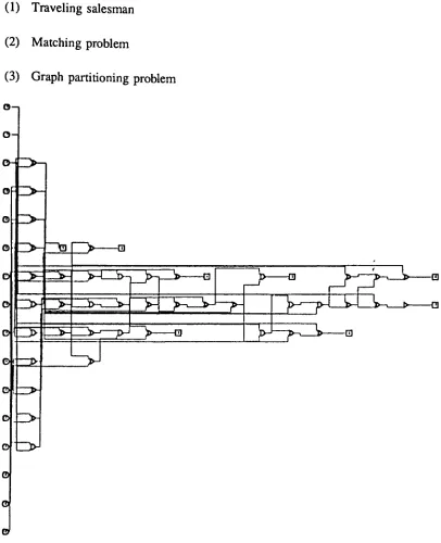
This multitude of energy minima exists because spin glasses in many situations are frustrated systems (see Figure 2.1). Frustrated systems arise when one spin, because of its interactions with other spins, is required to be in two different states. In Figure
2 2
+
3
4
+
3
+
4
[image:27.552.129.432.432.563.2]( a )
( b)( c )
18
2.1 a
"+"
labelling an edge (bond) represents the fact that the interaction of the bond tries to align the spins while a "-" sign means that the bond tries to anti-align the spins. In Figure 2.2 you will find the calculation for the energy of each of the possible states of the four spin system. Notice how there is only one ground state for the non-frustrated systems (a and c) while there are 2 ground states for the non-frustrated system (b). (Note: We do not consider the state that has all of its spin values reversed in the count of ground states - they are ground states because of the global spin-flip sym-metry of the energy function.) Thus, we see with a very simple system how frustration generates multiple ground states. Notice also that the ground state of the frustrated system is larger than the ground state of a corresponding non-frustrated system. One last comment should put this all into perspective. As is well known from biology, neurons can have excitatory and/or inhibitory connections. By allowing the Jjj'S to be(a)
(b)(c)
+1+1+1+1
-4
-2
0+1+1+1-1
0-2
0+1+1-1+1
0 0 0+1-1+1+1
0 0 0-1+1+1+1
0-2
0+1 + 1 - 1 - 1
0-2
+4
+1-1+1-1
4
+2
0 [image:28.553.126.386.428.591.2]+1 - 1 - 1 + 1
0+2
-4
both positive and negative we can create a frustrated system. Immediately it is seen
that the inhibitory and excitatory connections will be modeled by having positive and
negative synaptic connections in our neural networks. This will in turn lead to a
frus-trated neural system.
2.3. Previous Work and Problem Specification
Now we are ready to restate our ideas in the language of neural networks. The
simplest way to do this is to describe briefly some of the past work done. Hopfield's
model [Hopfield84] was the first to extract the analogy between magnetic systems
(spin glasses in this case) and neural networks. His approach was to form a
differential equation that, when solved, gives the state of each neuron at any given
time. Hopfield analyzed a model network using zero temperature (Le. noiseless)
Glauber dynamics. Little [Little74], 10 years before, analyzed a model using finite
temperature Glauber dynamics. In each of these models we define the Hamiltonian
(Le. the energy function) as:
(2.8)
As before Jii = 0
1 N N
E = - -2 ~~~ ~ J ..IJ S· S·I J
i=lj=l
and Jij =Jji . This is the Hamiltonian for an infinite range spin
glass where each spin interacts through the random exchange Jij' Both models when
analyzed used local learning [Gutfreund85]. Local learning rules specify that the
exchange interactions Jij (Le. the synapses) are modified only through the activity of
neuron i and neuron j but not on any extended group of neurons.
Recently, it has been discovered that nonlocal learning rules lead to error free
20
traditional equilibrium statistical mechanics (i.e. the description of systems at or very
near thermodynamic equilibrium) is not adequate. Normal systems at a finite
tempera-ture (in neuronal language, a system with noise) are ergodic. Ergodic behavior
con-demns the system to sample ALL of its possible states in a finite amount of time
irrespective of its initial state. Hence, with ergodic behavior the operation of an
asso-ciative memory fails. There are two possible ways out of this dilemma: the first is that
a system exhibits non-ergodic behavior for a time long enough for associative recall to
take place. Secondly, we can have cooperative behavior that will restrict the possible
network states to a limited set of states indefinitely. In the case of spin glasses we see both of the above situations. We shall call states that relax on time scales beyond
plausible observation times, metastable (i.e. they will relax to the minimum value of
the free-energy but only after a long time).
2.4. Theoretical and Conceptual Development
The technique that will be used throughout this thesis is called the "replica
method". This is a very sophisticated technique that will require much elaboration
before it can be properly justified, used and analyzed. Let us begin our discussion by
studying a system that is described by a set of statistical variables Sj. Also, assuming the system is random, we will need to specify a set of variables {x} that describe the
randomness of the system. Ifthe fluctuation time for the random variables is less than the observation time, then the system progresses to a state of thermal equilibrium. In
this case the usual techniques in equilibrium statistical mechanics can be used.
random variables of the system. For example, for the free-energy and the partition
function (i.e. the function from which we can derive ALL thennodynamic properties)
we have:
F = -T In [Z {x}]av (2.9)
Z [{x}] = Traces exp [-E {x, S;}/T] (2.10)
In the above fonnulas, T stands for the temperature while the Trace (Tr in future
equations) is over all possible spin configurations. (Note: Later we will see that the
free-energy is our "energy-function" in the noisy case.) The above average is called an
annealed average. To reiterate, an annealed average is only possible to perfonn if the
random variables participate in the dynamics of the system in the same manner as the
spins. As was discussed earlier, spin glasses relaxation times are much greater than
the observation times. This makes the above averaging technique inappropriate. The
proper averaging technique is called quenched averaging. In this scheme, the random
variables each take on a unique value as the statistical variables (i.e. the spins)
fluctu-ate. The question arises as to what should be averaged. In thennodynamics we have
two types of variables: intensive and extensive. An intensive variable is independent
of the size of the system while extensive variables are dependent on the "size" of the
system. By considering the following system [Brout59] we shall see that the size of
the system plays a dominant role in the averaging process. Now consider that a large
system is broken up into a collection of macroscopic systems each of which has its
own set of random variables. Also, assume that the interaction between each
subsys-tern is negligible. We can then calculate the (nonnalized) average of any extensive
22
number of subsystems grows, the above average will approach the average of an
extensive variable over all choices of {x}. Let us use the magnetization per spin Mas
an example:
M{x} - [M]av ~ 0 (for N ~ 00) (2.11)
Any system that satisfies the above equation for any set of random variables is called
self-averaging.
I state without proof that if we calculate the free-energy density f (i.e. the free
energy per spin) in this case we get a Gaussian distribution with width N112
[Binder86] :
Pif) oc exp{-Nif - [f]av)2/(2(/1/ )2)}
Ifthe annealed average of f is calculated then we get:
(2.12)
Fann = -
~
In[Z]av = [f]av+
(/1/)2([, (2.13) It would be expected that In [Z]av would give [f]av' But in this case we get anaddi-tional term. How can all this be viewed physically? We know that averaging over the
partition function will not work. For statistical mechanics to be of any use, we need a
free-energy function that will give us the ability to calculate the thermodynamic
pro-peTties of the system. But for this to be true, no large fluctuations of the free-energy
function can take place. So the proper quantity to be averaged is the free-energy func-tion, NOT the partition function. On a technical note, this is where the problems
begin. Averaging the partition function is a reasonable job but when dealing with the
logarithm of the partition function (i.e. the free energy) the job becomes much more
difficult A way around this is to use what is called the replica method. More on this
Let us return to the concept of ergodicity. We saw earlier that if ergodicity is present an associative memory cannot function. As is well known in Physics, any sys-tern, when noise (T >0) is present, will be ergodic. We discussed the possible solu-tions to this problem earlier. In spin glasses many states can be found that have the minimum value of the free-energy (these will be our retrieval states for a neural net-work). Most systems that exhibit broken ergodicity have low-lying states that are related by some symmetry of the Hamiltonian (Le. the energy function). This is not the case with spin-glasses. They exhibit what is called accidental degeneracy which is manifested from randomness and frustration. Before discussing the "replica method", there is one last important concept to discuss. Some means of labelling the multitude of thermodynamic ground states must be found. In Physics the most common way of labelling these states is by giving the average magnetization. In neuronal language this would be the overlap between the network state and a stored pattern.
The replica method is based on the formula [Binder86, Amit89]:
lim Zn - 1 = 1nZ
n~O n (2.14)
Immediately, one can see that the difficulty in averaging 1nZ is replaced by averaging
24
Assume that the energy of the system is E( {x} ,(S}), where {S} represents the spins of
the system and {x} represents a particular set of random variables.
zn({x}) = (Trs exp[-~E({x},{s})])n
= Trsl exp[-~E({x},{Sl})]) '" Trsft exp[-~E({x},{sn})]
= TrSl ....,sft exp[-~({x },(Sl, ... ,sn })],
where
(2.15)
n
~({x},(Sl,... ,sn}) =
L
E({x},(Sa}) (2.16)a=l
This is the energy of a system of n • N spins (i.e. each replica is a collection of N
spins). Once an explicit representation is known for the partition function then the
averaging over the random variables is carried out. At this time two paths could be
taken. The first is to continue with a general discussion of the replica method; the
other to relegate any further discussion of the method until the actual calculations.
The latter approach will be adopted here.
One of the goals of this thesis is to understand the workings of a neural network
that uses nonlocal learning. Thus, a nonlocal learning rule will be introduced and then
analyzed to determine its behavior as an associative memory. Another goal of this
thesis is to give a statistical mechanical treatment to a common combinatorial
optimi-zation problem. Here graph q-partitioning will be analyzed using the full power of
statistical mechanics and the replica method. Lastly, extensions of the use of statistical
mechanics to Ramsey numbers, graph coloring, and other optimization problems will
Earlier, it was stated that we can use an overlap parameter to distinguish retrieval
states (Le. states with minimal free-energy). In general situations, more than one parameter (generally called order-parameters) will be needed to specify retrieval states.
By generating the free-energy function, we shall be able to determine the set of
order-parameters (actually we will determine the equations for the order-order-parameters). These
equations are the equations for the extrema of the free-energy.
During the analysis we will have to be conscious of the presence of not only fast
noise (Le. noise generated by non-zero temperature) but also of slow noise (Le. noise
generated by small random overlaps of the pattern being retrieved, with all other
pat-terns stored in the network). The replica method can be used to determine the size of
the basin of attraction around each pattern stored in the network. These sizes are used
to determine which network states, in the presence of noise, will be attracted to the
stored patterns - associative recall.
A quantity that will be important throughout is <X =pIN, where p is the number of stored patterns in the network and N is the number of neurons in the network. It
will be seen that there is a value <Xc above which no retrieval takes place (Le. system
is ergodic). Below this value, spurious states, as well as stored patterns, will arise.
But, as more noise is introduced, these spurious states will be destabilized and thus the
system will have relatively good retrieval properties. So, as should be apparent, a
study of a network must be undertaken in the realm of no noise (T ~ 0 or
CHAPTER 3
ANN AND NONLOCAL LEARNING
3.1. Learning Rules
As discussed earlier, nonlocal learning rules deal with the activity of a collection of neurons not just two neurons. There seem to be two major arguments against using nonlocal learning rules: (1) no strong evidence has been found indicating that such nonlocal effects are seen in biological systems and (2) their introduction complicates any analytical study of an ANN. When dealing with artificial networks, any concern about biological plausibility can be disregarded. Even though no evidence for nonlocal learning has at present surfaced, it seems reasonable that there could be situations deal-ing with more abstract operations of a biological neural system which could involve some type of nonlocal learning. All local learning networks have difficulty learning correlated patterns. The overlaps between patterns can be specified by use of the matrix:
N
C~v ==N-1L~f ~t
i=l
(3.1) where Jl and veach range from 1 to p. The C~v generate an internal static noise which is the main reason that local learning rules encounter difficulty with correlated patterns. These overlaps effectively flip spins away from the original pattern (i.e. ori-ginal pattern is randomized). Let us look at the case where p is finite whileN is very large (---t 00 in the thennodynamic limit) and the patterns are uncorrelated. The
lative overlap is (choosing pattern 1 arbitrarily)
C -1 N J:1 P J:v
total = N
L
~iL
~ii=1 v=1
(3.2)
Equation (3.2) is a sum of Np bits of +1 and -1. Since the stored patterns are
uncorrelated, this is a one-dimensional random walk of Np steps. It is well known in
Physics that the mean square distance of a random walk from a preset origin is XL
where X is the number of steps andL is the step length. So, in this case we obtain
that the mean square distance of the walk is 0 ("pIN). In the case that <X =P IN is finite (Le. p and N both large) there exists a value <Xc above which there is a
break-down of associative recall. In all Hopfield style of networks with local learning rules, <Xc is always less than 0.14. This means that in a network of 100 neurons only 14
pat-terns could be stored and retrieved with any certainty.
3.2. Personnaz Model
Personnaz [Personnaz85] discussed nonlocal learning rules that can be used to
suppress the effects of overlaps between correlated patterns. The model he discussed
was based on the solution of the stability equation
~J.. J:~=A.J:~
~ I} ~I ~I
j
where i ranges from 1 to N and J..l ranges from 1 top .
(3.3)
These equations guarantee the
stability of an arbitrary set of stored patterns. The solution of Personnaz was the
J .. = N-1", ~~ ~y (C-1) IJ ~"" "'J ~v
IJ.,V
where C~v is the overlap matrix as defined earlier.
3.3. Noiseless Dynamics
28
(3.4)
In the noiseless case a particular network state (Le. the state ofN spins) is
con-sidered stable if the spins are each parallel to their respective local fields. To be pre-cise, the following relationships must hold:
Sj = sgn(hj )
h· = '" J ..1 ~ IJ S·J j
Let us now check the stability of the patterns in this model,
1:
Jjj~r
=
1:
N-1f
~? ~J
(C-1)av~r
j j a,v
- N-ll..~JJ.NC (C-1)
-
L""
~V ava,v
(3.5)
(3.6)
(3.7)
This shows that the stored patterns are eigenvectors of the synaptic matrix with
eigen-value of 1. Any pattern that is orthogonal to these patterns has an eigeneigen-value of O.
Now, to check the stability of a stored pattern, assume that the network is in the state
~~. Equation (3.5) now becomes,
~r
=sgn[7
Jij~J'
]
(3.8)the noiseless case.
3.4. Self-Coupling in Personnaz Model
A sufficient condition for the existence of an energy function is that the
interac-tions are symmetric [Amit89]. The necessity of an energy function is easily justified.
Given an energy function, the network is guaranteed to asymptotically drift to a fixed
point attractor. Inherent though unsaid in the condition is that Jii must be O. This
requirement is found to be true in the noiseless case and the noisy case. The simplest
example of this is in the noiseless asynchronous dynamics case. Asynchronous
dynamics involves the updating of only one spin per unit time interval. Consider the
energy function:
where the Jij's are arbitrary.
is changed from Sk to -Sk.
1
E = - - ~ J.. S· S·
2 .~ . IJ I J I.J.I*J
Let us calculate the change in E
(3.9)
when a single spin Sk
M = Sk ~ ljkSj
+
Sk ~ JjkSj (3.10) j.j~ j.j*kRemember, in Physics the dynamics of a system must be such that the energy of the
new state must be lower than the preceding state (at T '# 0 this must be
supple-mented). From equation (3.10), we see that the change will occur only if the first term
on the right is negative (i.e. the local field at site k is anti-parallel to the spin). Since
the Jij are completely arbitrary, there is no a priori way of knowing the sign of the
second term on the right. Thus a spin flip may not reduce the energy as required. If,
however, lkj = ljk E will be reduced on any spin flip and we can properly associate
30
condition for the existence of an energy function. At this point it is easy to see why we require Iii = O. Assuming that Iii ~ 0, then we would have a term in the expres-sion for M that contained S{ If this tenn were present, it would automatically be non-zero since
sl
is always 1. Thus the sum would no longer represent the local field at Sk' The importance of all of this is that any learning rule that has non-symmetric synaptic coefficients cannot be described by an energy function and thus the analytical techniques of statistical mechanics cannotbe used.It must be understood that a network with self-coupling is viable and can be stu-died through both simulations and analytical techniques. If the goal is to discard net-works which do have self-coupling, then a dynamic reason must be specified. Now in any neural network we are concerned with the basin of attraction of a pattern. The concept of a basin of attraction is the following:
A basin of attraction around a stored pattern represents the set of states near a stored pattern that willbe attracted to the stored pattern by the dynamics of the network.
Now in the case of the Personnaz model, the following will show that the effect of self-coupling is to reduce the size of the basin of attractions of the stored patterns. Consider the case where the network is in a state that corresponds to a stored pattern
{;f} except for one spin Sl' Then equation (3.5) reduces to:
S1= sgn(hI)
= sgn
[L
I 1j;j
+
I 11 S1]
j(#:1)
= sgn
(~f
-
J11~f
+
J11 S1 ) (3.11)The rule for constructing synapses allows us to rewrite equation (3.4) in a much more instructive form. First, calculate the mean ofJii.
=N-1
L,
(C-l)~V r~ ~r ~t]N-l
~,v
t
I=N-1
L,
(C-l)~V N C~vN-l~,v
=a (3.12)
At this stage we cannot use this result in equation (3.4) without proving that any varia-tion from the average is small (for large N).
(3.13)
oc ..JIN-3 - N-21
Thus the fluctuations around the average value of
a
are O(N-1). So for large N, thefluctuations are small and we can replace Jii with its average value in equation (3.4). Equation (3.4) now becomes:
S
1
oc sgn((1 -
a)~f
+
a S1)
(3.14)Looking at equation (3.14) we immediately see that if
a
> 112 the configurations S1=
~f and S1=
-~f are stable. Thus, the maximum capacity of the Personnaz32
3.5. Non-local Learning Model with an Energy Function
By adding the restriction that j '# i in equation (3.6), our work will be greatly simplified since we can now write an energy function for the network. Our energy
function will be:
where
1
E =--~2~J .. S· S·
IJ I J I,J
J .. = N-l~ ~J.l. ~y (C-1)
IJ ~ ~l ~J J.l.V
J.1,V
CJ.l.V =N-l~~J.l.~Y~~l ~l
i
(3.15)
As with the Personnaz model, the following relationships hold for the attractors of the
network:
Si = sgn(hi) (3.16)
(3.17) h·I = ~~ J .. S·IJ J
j,j*,
As discussed earlier, at finite temperature (T) the energy function cannot be used to find the attractors of the network (i.e. the ground states). The proper function is called
the free energy, which contains not only the energy function, but the entropy and the
temperature. So, at finite temperature the general formula for the free energy is:
F = -j3 InTr{Si} exp (-j3E ), j3 = liT (3.18)
Notice how the expression for the energy has the 1;; term while the equation for hi
does not. Calculating as done for the Personnaz model we find that
(3.19)
dynamics of the problem. To fonnally eliminate the diagonal tenns from the energy,
we specify the synaptic coefficient as Jij(1 - Bij). In the thennodynamic limit
(N ~ 00) we can rewrite this as Jij - o.Bij. Consider the eigenvalue equation dis-cussed earlier for the Personnaz model. This equation rewritten using the new fonn
forJ ..IJ is
~ (Iij -
aB
ij ) ~r = (1 - a.) ~r (3.20)j
Thus, stored patterns are eigenvectors of the synaptic matrix with eigenvalue 1 a.,
while patterns orthogonal to them have eigenvalue of-a..
3.5.1. Connection with Hopfield Model
Let us make the following decomposition for Si:
Si = ~ a~ (~r
+
1)+
BSi~
The pattern {BSi } is orthogonal to all embedded patterns. Inother words:
Now a measure of the order in the system is conventionally given by
(3.21)
(3.22)
(3.23)
These are used to parametrize the attractor distributions at finite temperature.
Tradi-tional nomenclature calls the m~'s order parameters. From a neural network
stand-point, they represent the average overlap of the network with a stored pattern. When
the number of patterns is much less than the number of neurons and the learning is
local, this is enough infonnation to parametrize what are called attractor distributions.
34
they can be properly used. Unfortunately, at memory saturation (i.e. p =:: N) even this
will not suffice.
Before continuing with the comparison of a Hopfield network and a nonlocal
learning ANN, let me clarify the idea of an attractor distribution. Throughout this
thesis we have always referred to a single attractor state (or its simplest version - a
fixed point). The notion of a single attractor state is only proper at zero temperature.
At non-zero temperatures the probability of a spin flipping away from a stable state is
non-zero (it is zero at zero temperature). We find in this situation a collection of
states close to a stored pattern with non-zero probability. Each of these states is
characterized by the fact that given the (average) overlap of the network state with a
stored pattern, we find that the network is trapped in the neighborhood of the stored
pattern. This collection of states is called an attractor distribution.
Since overlaps are tangible quantities, let us see if we can find a relationship
between the m~ and the a
w
Crudely, we can think of the a~ as the network overlapswith the stored ORTHOGONAL patterns and not the original patterns. Multiply
equation (3.21) by ~r and then sum over all i. We obtain the following:
L
Si ~i' =L L
a~ ~r ~i'+
L
BSi ~i'i ~ i
Using equation (3.22), the right-hand side of equation (3.24) becomes:
L L
a~ ~r ~i'i ~
Now using equation (3.23) and equation (3.25), equation (3.24) becomes:
mvN =
L L
a~ ~r ~i'i ~
(3.24)
(3.25)
(3.26)
C defined in equation (3.1). Thus we obtain:
mvN =
L
a~ N C~v (3.27)~
Now, multiply both sides of equation (3.26) by (C-1)pv and then sum over v. Thus we can rewrite equation (3.26) as:
L
(C-1)pv mv=
L
a~ (C-1)pv Cv~v ~,v
(3.28)
With the relationship between a~ and m~ established, let us rewrite the local field
equation hi and the energy function in tenns of the "overlap" parameters.
h·I = ~~ J ..IJ S·J
j,j"*i
= ~~J ..IJ S· -J J ..II S·I
j
=
L
N-1L
~r ~J (C-l)~vSjj IJ.,V
=
L
~r (C-l)~v mv~,v
- ~ J:~ a - J .. S·
- ~ ~l ~ II I
~
::: ~~~lJ:~ a -~
a
S·I
~
=
L
~r a~ -a(L
a~ ~r+
BSi )~ ~
= (l -
a)L
~r a~ -a
BSi~
Now, let us rewrite the energy function:
36
1
E = - -~ J .. S· S·
2~ I} I }
I.}
1
=--~2~h· S·
I I I
1
=
--2L
~f a~ Sj -LJ
jj S?~ j
Using equation (3.23) we can finally write:
N
E =-2La~m~
~
The corresponding equations in the Hopfield case are the following:
h·I = ~~~IJ:~ m -~
a
S·I ~(3.30)
(3.31)
(3.32)
N
E =
--L
(m~)2 (3.33)2 ~
Immediately, one can see that equations (3.29) and (3.30) are an advantage over (3.32) and (3.33). Consider the situation where Si = ~l. In the case of the m~'s we obtain
m~ - Ol~ = (C-l)l~ which is O(lI,,[N), no matter how the patterns are correlated. On
the other hand, a~ = Owregardless of the correlation of the patterns.
3.5.2. Global Minima of E
Consider the local fields of the configuration Sj = ~f. They are:
(3.34) For stability of all the patterns we must have Jjj :::;; 1. We will now prove that
L
JiJ
= N-2L L L
~f ~J ~1 ~}' (C-l)~v (C-1),/0j j ~.v ,/.0
= N-1
L L
~f ~1C vo (C-l)~v (C-1)yO=N-1
L L
~f ~1By'Y (C-l)~y~.y 'Y
= N-1
L
~f ~l (C-l)~y~.y
=Jii
Since this relationship holds for i=1,2,...,N we have: J .. - J.7II II = ~~J.fIJ ~ 0
j.j~
Immediately from equation (3.36) we have that 0 ~
lu
~ 1 for i=I,2, ...,N.(3.35)
(3.36)
Combining
this with equation (3.34) we see that the patterns will be stable for all p < N. Let us consider the following formulation for E. Define the quantity to be:
[ ]
112 /). = ~ (BSj)2
This is the Euclidean distance between the vector (N-dimensional)
(3.37)
{Sj} and the
p-dimensional subspace spanned by the patterns. Squaring equation (3.21) and then
summing overi we obtain:
L
S? =L «L
a~ ~f+
BSj)(Lay~t+
BSj))j j ~ y
=
L (L
a~ ~fL
ay ~t+
L
a~ ~f BSj+
L
ay ~t BSj+
(BSj)2)j ~ y ~ y
Using equations (3.22) and equation (3.28) we obtain:
N =
L (L
a~ay ~f ~l+
(BSj)2)j J.l.,y
Multiply equation (3.28) by ~f~l and sum over v and i to obtain:
L L
ay ~f ~t =L L L
(C-l)y~ m~ ~f ~ly j y j
~-=
NL L
(C-l)y~ m~ C~yy ~
=N m~
(3.38)
(3.39)
38
After all this we can finally give the final fonn of equation (3.39):
N =
NL
a~ m~+
(6Si)2 (3.41)~
Notice how the first tenn on the right is the expression for the energy function. Thus,
we can rewrite the energy function in tenns of the Euclidean distance between the
space of network states and the space of patterns.
N 1).2
E = +
-2 2 (3.42)
What has this refonnulation given us? It immediately shows that the p patterns are
global minima of E (they all have I).= 0). Unhappily, states that are linear
combina-tions of the patterns, are also global minima ofE (Le. these are spurious states of the
dynamics). Kanter [Kanter87] has shown that the probability for large N for the
occurrence of a state that is a linear combination of patterns vanishes asN ---7 00 as:
The last topic to be discussed with this fonnulation is to find the value for ac . Our
sole change of the Personnaz model is to remove the
.i
= i tenn in the sum for thelocal field hi. Let us redo the calculation for finding ac We can then immediately
rewrite equation (3.14) without theJ11
S1
=
sgn[(1 - a)~f] (3.43)3.6. Simulations of Network
CHAPTER 4
REPLICA METHOD AND GRAPH PARTITIONING
4.1. General Information
It is well known that spin glasses on random lattices with finite connectivity are
closely associated with combinatorial optimization problems such as graph partitioning
[Fu86, Mezard85, Kanter87]. There is considerable formal understanding of
infinite-ranged (Le. all spins interact with all other spins) spin glasses. Many physical and
conceptual problems still arise but they are not relevant to this discussion. Finite
con-nectivity is just a statement that a spin is connected to only a subset of all spins. A
random lattice is specified by a collection of interactions that are random in sign and
generally different in magnitude. In the case of an associative memory, as discussed in Chapter 3, these random interactions would give rise to the stored patterns. It is the
purpose of this chapter to solve the q-partitioning problem.
4.2. Problem Specification
In general, graph q-partitioning (Le. a graph is partitioned into q equal parts) is a
NP-complete problem, Le. no known algorithm can guarantee to find the absolute
optimal solution in polynomial time. The particular problem to be studied in this
chapter is the following: take a graph specified by G(V ,E), where IV I = N is an integral multiple ofq. The graph is then to be partitioned into q equal groups of
ver-tices such that the intergroup edges (i.e. connection between two verver-tices) are
ized. In this case an Ising spin system will not be used. A Potts spin system will be utilized instead. The energy function in this case is:
2
E = - -~T..(qB - 1 )
q ~IJ SIS}
l<j
where Bis called the Kronecker delta symbol and has the following property:
(4.1)
ifs·I
=
s·J ifs·I :F- s·J(4.2)
The Jij 's represent the randomness of the system. In the graph partitioning case we
specify each edge byJij such that:
J .. = { J
IJ 0
with probabilityp
with probability 1 - p
(4.3)
This probability distribution can be explicitly written as:
p(Jij)
=
pB(Jij - J)+
(l - p) B(Jij)In this case Bis the Dirac delta function which is defined as follows:
(4.4)
ll(x - a)= {
~
ifx :F-aifx
=
a(4.5)
The Dirac delta function is more properly defined in terms of an integral equation, such as:
Jf
(x )B(x - a)dx=
f
(a ) (4.6)42
spins as discussed earlier. They will be considered to be one of the q-roots of unity. In particular choose:
Si E {exp(21tin/q) In = 0,1,...,q - I} With this representation for Si we can specify the constraint as:
~ S[
=
0 for r=
1, 2,...,q - 14.3. Cost Function
(4.7)
(4.8)
For a Statistical Mechanics treatment to be fruitful we must determine a cost function to be minimized and its connection to the energy function. We already know that we want to minimize the number of connections between partitions. It will tum out that this is easily translated into a formal cost function. Let us rewrite the energy function taking care to specify all possible situations for the combinations of i and j .
The expanded energy function is:
E = -(q - 1)
r
~
+ ... +
~
]
iij / q~,jEV1 i,jEV,
+
[~
+ ... +
~
+
+
~
+
+
~
]
iij / qiEV1 iEV1 iEV, iEV,
jEVz jEV, jEV1 jEV,_l
Since the only contribution to the sums will come when iij =J we can write:
E = -p(q - I)JN(N - 1)
+
2Ciq
where C is defined as:
(4.9)
(4.10)
C
=.E...
+
N(N - l)p(q - 1) (4.11)2J 2q
(4.13)
edges.
4.4. Free Energy Expression
Starting with equation (2.14) we can specify the average of
zn
where Z is the ..one" -particle partition function. For the average we have:- - N n
Zn =Tr {sa}
n
fdlijP (Jij)exp(-~I:Jij(Bsjast - 1)) (4.12)i<j 0.=1
Using the probability distribution for the interactions, equation (4.4), we obtain:
zn
= Tr{sa}n
~
expr~
±(qBsjast - 1)]+
(1 - P)]1<]
r
l
q 0.=1_ ,N(N-1)/2' N [
[~
n ]]- (l - P
r
Tr {sa}exp~.ln 1+
PoexpI:
(q Bsjast - 1)l<j q 0.=1
where Po is defined as P /(I-p ). Remember at each stage of the analysis the
con-straint, equation (4.8), must be satisfied. To indicate this the trace has had a prime
appended to it. At this stage the expression for the average of the partition function is
still too cumbersome. To reduce the complexity of the partition function and to reach
the point where we can explicitly use the constraint, expand the exponential and the
natural logarithm into their power series form. I will detail the steps here since the
techniques and philosophy are an integral part of the analysis. For simplicity define:
~ n
X =
I:
(qBs.as.a - 1)q 0.=1 I J
(4.14)
Expand the natural logarithm and then the exponential in their power series form:
00 (-li+1pO
I
In(1 +Poexp(x)) =
I:
I exp(lx)00 (-I)I+1POI [ 00 Ikx k ]
=L
1+L
-1=1 I k=1 k!
00 (_I)I+1p 1 I k k
= In(l
+
po)+
L
0 XkJ=1 I k!
For the average of the partition function we now have:
-
IN [
00 ( 1)1+1pl I xk ] )Zn = (l - P)N(N-l)/2 exp ~. In(l
+
Po)+
L -
0 _k_,_1<) k,I=1 I k.
= (I - P
yV(N-IlJ2
exp { N (N Z- 1)In(I
+
Po) }I
N [00 (-I)I+1Pb
I k ] )x exp
L L
- x
ki<j k,I=1 I k!
Ifwe define the following coefficients we can simplify the formula:
00 (_1)1+1 Ik
C - ~ pI
k - ~
k
O---k'
1=1 •
Ifx is now written out explicitly the following formula is obtained:
-
{N(N-l)}
Zn = (l - p )N(N-l)/2exp 2 In(l
+
Po)x expli:
[~]kCk~.
[±(qOSiUSt _
1)]k) k=1 q 1<) a=144
(4.15)
(4.16)
(4.17)
(4.18)
Now from the properties of the natural log and the exponential functions we have:
(1 - P
yV(N-llJ2{
N(~-I)
In(1+
Po) } = 1 (4.19)the sum on i and j to include all combinations ofi and j. By multiplying by 112 we can easily adjust for the inclusion of tenns when i >j. The analysis is slightly more involved to remove the self-coupling terms (i.e. when i = j). The correction term is
calculated using the following idea: calculate the general tenn when i = j and change the sign of the exponent. This tenn is easily seen as:
Correction_term = exp{_N
~ [~]\q
-l)k
nk}
(4.20) 2k=l qWe are now ready to write a form of
zn
in which the effect of the constraint and the limit as n ~ 0 can be easily seen:(4.21)
A variation, but completely equivalent version of equation (4.8), can be used to sim-plifyequation (4.21). This version is the following:
f
[<>so..so.. -1.]
= 0 (4.22)• • I J q
I.}
The relationship between the energy of the system and the free-energy of the system
is:
F = E -
~
(4.23)where S is the entropy of the system. In the limit that ~ ~ 00 we immediately see
that the free-energy F and the energy E are equal. Thus we can rewrite our cost
(4.24)
46
C -
-
N (N - l)p (q - 1)+
Iim -F2q ~~21
No matter what form we have the free-energy in, to calculate any values we
must, in the final analysis, calculate a sum over all possible spin configurations (Le.
perform the trace). There is a spin representation in which we can replace the delta
function with a sum over spin variables. This representation is:
f(;,1
q Bs/sj = 1
+
L (SiSj*)r r=lThe formula for the free-energy in terms of the partition function is:
1
F = --lnZ
~ Ifwe use equation (2.14) we obtain:
1
f,
1
00
1
[~]k
N[
n f(;,1 *]k )
I
-~F = lim- Tr{S,,}exp
L-
ckL L
LS/J.St - 1n~On k=22 q i,j a=lr=l
Notice that the first exponential in equation (4.21) is 1 in the limit when n ~ O. (4.25)
(4.26)
(4.27)
It was necessary in Chapter 2 to rescale J so as to guarantee that the local fields
would not be dependent on N. In that case, from a formal standpoint this guaranteed a sensible thermodynamic limit (Le. N ~ 00). Since
ck
is 0 (1) with regard to N, a rescaling ofJ ~ J/fN
will lead to a sensible limit. Each term in the sum making upthe free-energy formula will be of 0 (lINk12). Therefore in the thermodynamic limit the first term in the series will dominate. In this case:
C2=
~po(1
+
por2 =~p(1-
p)The double sum on i and j can also be rewritten as:
n n q-lq-l N
=
2N'L
'L 'L 'L 'L(SjU)'
(S?,/
r1a=l,=lr=1 j=lu<:y
where
![Figure 1.1: The construction for the exclusive or (xor by the route [A +B H...,[A·B]] [Amit89].](https://thumb-us.123doks.com/thumbv2/123dok_us/110246.10258/15.553.92.442.78.224/figure-construction-exclusive-xor-route-b-h-amit.webp)
![Figure 1.2: A single layer multi-perceptron [Amit89].](https://thumb-us.123doks.com/thumbv2/123dok_us/110246.10258/16.555.108.381.48.265/figure-a-single-layer-multi-perceptron-amit.webp)
![Figure 1.3: A multi-perceptron closed on itself to fonn an ANN [Amit89].](https://thumb-us.123doks.com/thumbv2/123dok_us/110246.10258/17.552.104.317.49.259/figure-multi-perceptron-closed-fonn-ann-amit.webp)
![Figure 1.5: Geometrical representation of the distance between pairs of network states [Amit89].](https://thumb-us.123doks.com/thumbv2/123dok_us/110246.10258/20.552.101.340.55.275/figure-geometrical-representation-distance-pairs-network-states-amit.webp)
![Figure 2.1: Three sets of four spins arranged on squares. The numbering is only for labelling purposes.(a) a ferromagnetic square; (b) a frustrated square - three aligning and one anti-aligning interactions; (c)a non-frustrated square - two aligning and two anti-aligning interactions [Amit89].](https://thumb-us.123doks.com/thumbv2/123dok_us/110246.10258/27.552.129.432.432.563/numbering-labelling-ferromagnetic-frustrated-aligning-interactions-frustrated-interactions.webp)
