https://doi.org/10.5194/angeo-37-263-2019 © Author(s) 2019. This work is distributed under the Creative Commons Attribution 4.0 License.
Validation and application of optimal ionospheric shell height model
for single-site estimation of total electron content
Jiaqi Zhao and Chen Zhou
School of Electronic Information, Wuhan University, Wuhan, 430072, China Correspondence:Chen Zhou ([email protected])
Received: 1 July 2018 – Discussion started: 12 July 2018
Revised: 18 March 2019 – Accepted: 28 March 2019 – Published: 26 April 2019
Abstract. We recently proposed a method to establish an optimal ionospheric shell height model based on the inter-national GNSS service (IGS) station data and the differen-tial code bias (DCB) provided by the Center for Orbit De-termination in Europe (CODE) during the time from 2003 to 2013. This method is very promising for DCB and accu-rate total electron content (TEC) estimation by comparing to the traditional fixed shell height method. However, this method is basically feasible only for IGS stations. In this study, we investigate how to apply the optimal ionospheric shell height derived from IGS station to non-IGS stations or isolated GNSS receivers. The intuitive and practical method to estimate TEC of non-IGS stations is based on optimal ionospheric shell height derived from nearby IGS stations. To validate this method, we selected two dense networks of IGS stations located in regions in the US and Europe. Two optimal ionospheric shell height models are established by two reference stations, namely GOLD and PTBB, which are located at the approximate center of two selected regions. The predicted daily optimal ionospheric shell heights by the two models are applied to other IGS stations around these two reference stations. Daily DCBs are calculated according to these two optimal shell heights and compared to respec-tive DCBs released by CODE. The validation results of this method are as follows. (1) Optimal ionospheric shell height calculated by IGS stations can be applied to its nearby non-IGS stations or isolated GNSS receivers for accurate TEC estimation. (2) As the distance away from the reference IGS station becomes larger, the DCB estimation error becomes larger. The relation between the DCB estimation error and the distance is generally linear.
1 Introduction
Dual-frequency GPS signal propagation is affected effec-tively by ionospheric dispersive characteristics. Taking ad-vantage of this property, ionospheric total electron con-tent (TEC) along the path of signal can be estimated by differencing the pseudorange or carrier phase observations from dual-frequency GPS signals. Carrier phase leveling or smoothing of code measurement is widely adopted to im-prove the precision of absolute TEC observations (Mannucci et al., 1998; Horvath and Crozier, 2007). In general, it is considered that the derived TEC in carrier phase leveling or smoothing technique consists of slant TEC (STEC), the combination differential code bias (DCB) of satellite and re-ceiver, multipath effects and noise. The DCB is usually con-sidered as the main error source and could be as large as several TEC units (TECu) (Lanyi and Roth, 1988; Warnant, 1997).
further developed this model into a single thin-layer model and proposed the standard geometric mapping function and the polynomial model. The single thin-layer model assumed that the ionosphere is simplified by a spherical thin shell with infinitesimal thickness. Clynch et al. (1989) proposed a mapping function in the form of a polynomial by assum-ing a homogeneous electron density shell between altitudes of 200 and 600 km. Mannucci et al. (1998) presented an ele-vation scaling mapping function derived from the extended slab mode. There are also many modified mapping func-tions according to the standard geometric mapping function. Schaer (1999) proposed the modified standard mapping func-tion using a reduced zenith angle. Rideout and Coster (2006) presented a new mapping function which replaces the in-fluence of the shell height by an adjustment parameter and set the shell height as 450 km. Smith et al. (2008) modified the standard mapping function by using a complex factor. Based on the electron density field derived from the interna-tional reference ionosphere (IRI), Zus et al. (2017) recently developed an ionospheric mapping function at fixed height of 450 km with dependence on time, location, azimuth angle, elevation angle, and different frequencies.
The ionospheric shell height is considered to be the most important parameter for a mapping function, and the shell height is typically set to a fixed value between 350 and 450 km (Lanyi and Roth, 1988; Mannucci et al., 1998). Birch et al. (2002) proposed an inverse method to estimate the shell height by using simultaneous VTEC and STEC observations and suggested the shell height is preferably a value between 600 and 1200 km. Nava et al. (2007) utilized multiple sta-tions to obtain a shell height estimation method by mini-mizing the mapping function errors; this method is referred as the “coinciding pierce point” technique. Their results in-dicated that the suitable shell heights for the midlatitude is 400 and 500 km during the geomagnetic undisturbed condi-tions and disturbed condicondi-tions, respectively. In the case of the low latitude, the shell height at about 400 km is suitable for both quiet and disturbed geomagnetic conditions. Jiang et al. (2018) applied this technique to estimate the optimal shell height for different latitude bands. In their case, the optimal layer height is about 350 km for the entire globe. Brunini et al. (2011) studied the influence of the shell height by using an empirical model of the ionosphere and pointed out that a unique shell height for whole region does not ex-ist. Li et al. (2018) applied a new determination method of the shell height based on the combined international GNSS service (IGS) Global Ionospheric Maps and the two meth-ods mentioned above to the Chinese region and indicated that the optimal shell height in China ranges from 450 to 550 km. Wang et al. (2016) studied the shell height for a grid-based algorithm by analyzing goodness of fit for STEC. Lu et al. (2017) applied this method to different VTEC models and investigated the optimal shell heights at solar maximum and at solar minimum.
In the recent study by Zhao and Zhou (2018), a method to establish an optimal ionospheric shell height model for single-station VTEC estimation has been proposed. This method calculates the optimal ionospheric shell height in or-der to minimize the difference between the estimated DCB and the DCB released by the Center for Orbit Determination in Europe (CODE). Five optimal ionospheric shell height models were established by the proposed method based on the data of five IGS stations at different latitudes and the cor-responding DCBs provided by CODE during 2003 to 2013. For the five selected IGS stations, the results have shown that the optimal ionospheric shell height models improve the ac-curacies of DCB and TEC estimation compared to a fixed ionospheric shell height of 400 km in a statistical sense. We also found that the optimal ionospheric shell height shows 11- and 1-year periods and is correlated to the solar activity, which indicated the connection of the optimal shell height with ionospheric physics.
While the proposed optimal ionospheric shell height model is promising for DCB and TEC estimation, this method also can be implemented to isolated GNSS receivers not belonging to IGS stations, if we can get the long-term observations and reference values of DCB from the isolated GNSS receivers. By considering the spatial correlation of ionospheric electron density, it is intuitive and practical to adopt the optimal ionospheric shell height of a nearby IGS station to the non-IGS stations. So whether an optimal iono-spheric shell height model can improve the TEC/DCB esti-mation of nearby stations needs to be verify.
The purpose of this study is to investigate the feasibility of applying the optimal ionospheric shell height model derived from IGS station to nearby non-IGS GNSS receivers for ac-curate TEC and DCB estimation. By selecting two different regions in the US (Region I) and Europe (Region II) with dense IGS stations, we calculate the daily DCBs of 2014 by using the optimal ionospheric shell heights derived from data from 2003 to 2013 of two central stations in two regions. We also try to find the DCB estimation error and its relation to the distance away from the central reference station.
2 Method
In the polynomial model, the VTEC is considered as a Tay-lor series expansion in latitude and solar hour angle, which is expressed as follows:
TV(ϕ, S)=
m X
i=0
n X
j=0
Eij(ϕ−ϕ0)i(S−S0)j, (1)
where TV denotes VTEC. ϕ and S denote the geographic
latitude and the solar hour angle of ionospheric pierce point (IPP), respectively; ϕ0 andS0 denoteϕ andS at the
center of the cover region of IPP in 1 day.Eij is the model coefficient, andmandndenote the orders of the model. A polynomial model fits the VTEC over a period of time. In our case, a VTEC model is generated over 3 h of time, therefore eight VTEC models are applied per day. DCB is considered as constant in one day. Since our analysis is based on long-term single-site data, we setmandnto 4 and 3, respectively. Huang and Yuan (2014) applied the polynomial model with the same orders to TEC estimation.
Based on the thin shell approximation, the observation equation can be written as follows:
TosPRN(ϕ, S)=TV(ϕ, S)·f (z)+DCBPRN, (2)
whereTosPRNis slant TEC calculated by carrier phase smooth-ing, the superscriptPRNdenotes the GPS satellite,DCBPRN denotes the combination of GPS satellite and receiver DCB, andzdenotes the zenith angle of IPP. According to Lanyi and Roth (1988), the standard geometric mapping functionf (z) is expressed as follows:
f (z)=1/cos(z) , (3)
z=arcsinRE·cosEl RE+h
, (4)
whereREdenotes the earth’s radius,Eldenotes the elevation
angle, andhdenotes the thin ionospheric shell height. Note thathalso affects the location of the IPP.
To estimate DCBs, the method above requires a definite thin shell height value. Conversely, if we get the daily solu-tions of DCBs, the optimal ionospheric shell height can be estimated. The optimal ionospheric shell height is assumed to be between 100 and 1000 km and is defined as the shell height with the minimum difference between DCBPRN and the reference values. This optimization problem can be writ-ten as follows:
min
100<h<1000mean(|DCBref−DCB|)s.t.T=8·E+θ·DCB, (5) where h is the daily optimal ionospheric shell height, DCBrefdenotes the vector of the reference values of DCBs,
s.t. is the abbreviation for subject to,T =8·E+θ·DCB is the matrix form of all the observation equations in one
day,T denotes the vector ofTos,E corresponds to the
co-efficients of the models and containsEij,DCB is the vec-tor ofDCBPRN,8is the coefficient matrix of E and con-tains(ϕ−ϕ0)i(S−S0)jf (z), andθis the coefficient matrix
ofDCB and contains only 1 and 0 s.E andDCB are un-known.
After the method above is applied to 11-year data, the es-timated optimal ionospheric shell heights can be modeled by a Fourier series, which is expressed as follows:
h (x)=a0+
k X
n=1
ancos
2nπ x
L +bnsin 2nπ x
L
, (6)
wherek is the order of Fourier series and is set to 40, an andbnare the model coefficients,xis the time, andLis the time span which is equal to 4018 d. The maximum frequency of the model is 40/ L≈0.01 per day, which corresponds to a period of 100 d. By the least-squares method, the model coefficients can be estimated.
This model can be applied to neighboring stations’ DCB estimations. Instead of fixed shell height, this model provides a predicted optimal ionospheric shell height. Note that, while in the establishment and application of the model, the VTEC model, mapping function and elevation cut-off angle are con-stant, all of them affect the optimal ionospheric shell height.
3 Experiment and results
The previous section introduced a method to establish a daily optimal ionospheric shell height model based on a single site with reference values of DCBs. To analyze the improvement of DCB estimation by this model for the reference station and other neighboring stations, we present two experiments to evaluate and validate this method by using IGS stations located in the US and Europe. To ensure the accuracy and consistency of DCB, we only select IGS stations with pseu-dorange measurements of P1 code, and whose receiver DCBs have been published by CODE.
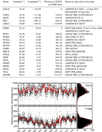
Figure 1.Geographical location of the selected IGS stations in the US region (Region I) and Europe region (Region II). The black tri-angle in each plot is the reference station.
for the other stations. In region I, the receiver type of GOLD was changed once in September 2011. The five selected sta-tions used four receiver types in 2014; TABV and PIE1 had the same receiver type. In region II, there are 9 receiver types for the 16 stations. The receiver type of PTBB has changed twice in 2006.
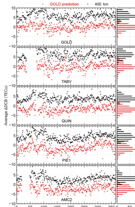
Figure 2 shows the estimated daily optimal ionospheric shell height of GOLD and PTBB during the period from 2003 to 2013. The left panel shows the variation in the daily opti-mal ionospheric shell height and the fitting result by Eq. (6). From the overall trend, the variations in daily optimal iono-spheric shell height for both stations appear as wave-like oscillations during the 11-year period. In the right panel, the statistical results are fitted by a normal distribution. The mean and the standard deviation (SD) of the normal distri-bution are 714.3 and 185.4 km for GOLD, respectively. The mean and SD values for PTBB are 416.4 and 184.1 km, re-spectively. At the end of 2010, a gap appears, because the DCB provided by CODE is simultaneously anomalous for both stations (Zhao and Zhou, 2018), and the data during this period are abandoned.
Figure 3 shows the amplitude spectra of the daily optimal ionospheric shell height of the two reference stations
esti-mated by the Lomb–Scargle analysis (Lomb, 1976; Scargle, 1982). As can be found in Fig. 3, the peaks correspond to 11-year, 1-11-year, 6-month and 4-month cycles. The amplitudes of 11- and 1-year cycles are more evident than other periods in both stations. As mentioned earlier, 0.01 per day is about the maximum frequency of Eq. (6). Higher frequencies would not be useful because of their small amplitudes. This result shows that the optimal ionospheric shell height of GOLD and PTBB is periodic, and the 40th order of Fourier series is suit-able for modeling its variation.
We establish two optimal ionospheric shell height mod-els for each region from the 40th-order Fourier series based on the 11-year data of GOLD and PTBB. To investigate the availability zone of the optimal ionospheric shell height model, we apply the models to the stations of each region as shown in Fig. 1 and Table 1. Based on the predicted daily optimal ionospheric shell heights in 2014 calculated by the model at GOLD or PTBB, each station is applied to estimate DCB separately in 2014 using Eqs. (1)–(4). The difference in DCBs in all stations in each region calculated using the optimal ionospheric shell height model at the reference sta-tions and DCBs provided by CODE is then compared to the difference in DCBs calculated using a fixed ionospheric shell height (400 km) and DCBs released by CODE.
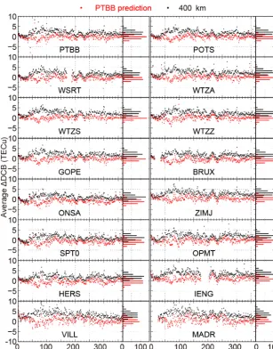
The results of this comparison are shown in Fig. 4. The panels for the stations are arranged by their distances to ref-erence stations, and this is also applied to Table 2; from the top panels to the bottom panels, the distance of the corre-sponding station to the reference station gradually increases. The left and right panels show the daily differences and the histograms of the statistical results in 2014, respectively. For all of the stations, the daily average differences of DCBs cal-culated using the optimal ionospheric shell height model are reduced compared to those using the fixed ionospheric shell height. For GOLD and TABV, the improvement is substan-tial; the daily average1DCB is close to zero. For the other stations, the median daily average 1DCB is negative, but smaller in absolute value than using the fixed shell height. This result shows the improvement of the model seems to be related with the distance to GOLD. Data gaps in the fig-ure correspond to days when data from that station are not available. Figure 5 is the same format as Fig. 4 and shows the results of Region II. Comparing to the results of fixed ionospheric height, Fig. 5 also indicates that the1DCB cal-culated using the optimal ionospheric shell heights at PTBB is on average smaller than that calculated using fixed iono-spheric shell height. Both Fig. 4 and 5 show that the accu-racy of DCB estimation can be improved using optimal iono-spheric heights from reference stations.
Table 1.Information for the stations.
Name Latitude (◦) Longitude (◦) Distance to GOLD Receiver type and service date or PTBB (km)
GOLD 35.42 −116.89 0 ASHTECH Z-XII3∼14 Sep 2011 JPS EGGDT 19 Sep 2011 TABV 34.38 −117.68 136.67 JAVAD TRE_G3TH DELTA QUIN 39.97 −120.94 619.55 ASHTECH UZ-12
PIE1 34.30 −108.12 810.51 JAVAD TRE_G3TH DELTA AMC2 38.80 −104.52 1159.09 ASHTECH Z-XII3T
PTBB 52.15 10.30 0 SEPT POLARX2 25 Jul–13 Nov 2006 ASHTECH Z-XII3T else
POTS 52.38 13.07 190.82 JAVAD TRE_G3TH DELTA WSRT 52.91 6.60 264.92 AOA SNR-12 ACT WTZA 49.14 12.88 381.28 ASHTECH Z-XII3T WTZS 49.14 12.88 381.28 SEPT POLARX2
WTZZ 49.14 12.88 381.28 JAVAD TRE_G3TH DELTA GOPE 49.91 14.79 401.51 TPS NETG3
BRUX 50.80 4.36 439.03 SEPT POLARX4TR ONSA 57.40 11.93 593.72 JPS E_GGD
ZIMJ 46.88 7.47 620.79 JAVAD TRE_G3TH DELTA SPT0 57.72 12.89 641.78 JAVAD TRE_G3TH DELTA OPMT 48.84 2.33 674.24 ASHTECH Z-XII3T HERS 50.87 0.34 705.38 SEPT POLARX3ETR IENG 45.02 7.64 816.64 ASHTECH Z-XII3T VILL 40.44 −3.95 1696.62 SEPT POLARX4
MADR 40.43 −4.25 1712.27 JAVAD TRE_G3TH DELTA
Figure 2.Variation in the daily optimal ionospheric shell height (black) and the fitting result (red).
values are reduced to 0.12 and 0.08 TECu, respectively; the root mean squares are reduced by 4.43 and 4.33 TECu, re-spectively. For Region II, the improvements in DCB estima-tion are the most obvious for WTZZ, with the mean value of1DCB decreasing from 2.34 to 0.02. We could note that
TABV and WTZZ station are quite close to the reference sta-tions in each region.
Table 2.Statistical results of mean and RMS of average1DCB in 2014.
Station Average1DCB (TECu) Average1DCB (TECu) Optimal ionospheric height Fixed ionospheric height
Mean RMS Mean RMS
GOLD 0.12 1.82 5.96 6.25
TABV 0.08 2.04 6.06 6.37
QUIN −1.60 2.31 3.91 4.19 PIE1 −1.38 2.50 4.46 4.84 AMC2 −2.12 2.75 3.09 3.53
PTBB −0.28 1.23 1.82 2.26 POTS −0.27 1.00 1.84 2.18 WSRT −0.41 1.14 1.65 2.10
WTZA 0.09 1.20 2.38 2.73
WTZS 0.14 0.99 2.48 2.76
WTZZ 0.02 1.14 2.34 2.65
GOPE −0.17 1.00 2.12 2.41 BRUX −0.42 1.12 1.86 2.13 ONSA −0.88 1.40 1.10 1.63
ZIMJ 0.48 1.17 2.87 3.13
SPT0 −0.84 1.40 1.14 1.67 OPMT −0.29 1.21 1.93 2.35 HERS −0.37 1.19 1.84 2.19
IENG 1.05 1.57 3.44 3.69
VILL 0.59 1.67 3.30 3.66
[image:6.612.51.281.92.548.2]MADR 0.66 1.71 3.50 3.86
Figure 3.Lomb–Scargle spectra of the daily optimal ionospheric
shell height.
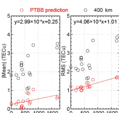
and the root mean square, respectively, with the distance to GOLD or PTBB. For all of the stations, the optimal iono-spheric shell height model improves the accuracies of DCB estimation compared to the fixed ionospheric shell height in a statistical sense; both of the absolute mean values and the root mean squares become smaller. For the optimal iono-spheric shell height model, the absolute mean values show a positive correlation with the distance to reference station GOLD or PTBB in each region, as well as the root mean squares. By using the linear regression, for Region I, the
ab-Figure 4.Comparisons of the average1DCB calculated using the
predicted optimal ionospheric shell heights (red dots) and those us-ing the fixed ionospheric shell height (black dots) in 2014 for sta-tions in Region I.
[image:6.612.50.282.96.566.2]Figure 5.Comparisons of the average1DCB calculated using the predicted optimal ionospheric shell heights (red dots) and those using the fixed ionospheric shell height (black dots) in 2014 for stations in Region II.
4 Summary
In this study, we implement and validate a method to trans-fer the optimal ionospheric shell height derived for IGS sta-tions to non-IGS stasta-tions or isolated GNSS receivers. We es-tablish two optimal ionospheric shell height models by the 40th-order Fourier series based on the data of IGS stations GOLD and PTBB in two separate regions. These two models are applied to the stations in each region, where the distance to GOLD ranges from 136 to 1159 km and the distance to PTBB ranges from 190 to 1712 km. The main findings are summarized as follows:
1. The optimal ionospheric shell height model improves the accuracy of DCB estimation compared to the fixed shell height for all of the stations in a statistical sense. These results indicate the feasibility of applying the op-timal ionospheric shell height derived from IGS stations
to other neighboring stations. The IGS stations can cal-culate and predict the daily optimal ionospheric shell height and then release this value to the nearby non-IGS stations or isolated GNSS receivers.
de-Figure 6. Relation of the accuracy for DCB estimation with the distance to GOLD. The red lines are the linear fitting results.
Figure 7. Relation of the accuracy for DCB estimation with the
distance to PTBB. The red lines are the linear fitting results.
pends on the quality of the optimal shell height model at the reference stations themselves.
Due to a requirement of this experiment, we only analyze two regions in midlatitude because of the insufficiency of long-term P1 data. We also ignore the orientation of isolated GPS receivers to the reference station.
Data availability. This study is based on data services provided by the IGS (International GNSS Service) and CODE (the Center for Orbit Determination in Europe). The data from the IGS stations can be downloaded from http://www.igs.gnsswhu.cn/index.php/Home/ DataProduct/igs.html (last access: 18 April 2019) (IGS, 2019) or the online archives of the Crustal Dynamics Data Information Sys-tem (CDDIS), NASA Goddard Space Flight Center, Greenbelt, MD, USA (ftp://cddis.gsfc.nasa.gov/pub/gps/data/daily/). The data
of the reference DCB can be downloaded from the online archives of CODE (ftp://ftp.aiub.unibe.ch/CODE/) or the online archives of CDDIS (ftp://cddis.nasa.gov/gnss/products/ionex/). The receiver type and service date can be obtained from https://cddis.nasa.gov/ Data_and_Derived_Products/CddisArchiveExplorer.html (last ac-cess: 18 April 2019) (NASA, 2019).
Author contributions. JZ and CZ designed the experiments and JZ carried them out. JZ developed the model code and performed the simulations. JZ and CZ prepared the paper.
Competing interests. The authors declare that they have no conflict of interest.
Acknowledgements. This study is based on data services provided by the IGS (International GNSS Service) and CODE (the Cen-ter for Orbit DeCen-termination in Europe). This work is supported by the National Natural Science Foundation of China (NSFC grants 41574146 and 41774162). Thanks also to Dalia Buresova and Max van de Kamp and two anonymous referees.
Review statement. This paper was edited by Dalia Buresova and reviewed by Max van de Kamp and two anonymous referees.
References
Birch, M. J., Hargreaves, J. K., and Bailey, G. J.: On the use of an effective ionospheric height in electron con-tent measurement by GPS reception, Radio Sci., 37, 1015, https://doi.org/10.1029/2000RS002601, 2002.
Brunini, C., Camilion, E., and Azpilicueta, F.: Simulation study of the influence of the ionospheric layer height in the thin layer ionospheric model, J. Geodesy, 85, 637–645, https://doi.org/10.1007/s00190-011-0470-2, 2011.
Clynch, J. R., Coco, D. S., and Coker, C. E.: A versatile GPS ionospheric monitor: high latitude measurements of TEC and scintillation, in: Proceedings of ION GPS-89, the 2nd Interna-tional Technical Meeting of the Satellite Division of The Institute of Navigation, Colorado Springs, CO, USA, 22–27 September 1989, 445–450, 1989.
Horvath, I. and Crozier, S.: Software developed for obtaining GPS-derived total electron content values, Radio Sci., 42, RS2002, https://doi.org/10.1029/2006RS003452, 2007.
Huang, Z. and Yuan, H.: Ionospheric single-station TEC short-term forecast using RBF neural network, Radio Sci., 49, 283–292, https://doi.org/10.1002/2013RS005247, 2014.
IGS: Data of IGS stations, available at: http://www.igs.gnsswhu. cn/index.php/Home/DataProduct/igs.html, last access: 18 April 2019.
[image:8.612.67.264.291.478.2]Klobuchar, A.: Ionospheric time-delay algorithm for single-frequency GPS users, IEEE Trans. Aero. Elec. Sys., AES-23, 325–331, 1987.
Komjathy, A.: Global Ionospheric Total Electron Content Mapping Using the Global Positioning System, PhD thesis, Department of Geodesy and Geomatics Engineering Technical Report NO. 188, University of New Brunswick, Fredericton, New Brunswick, Canada, 248 pp., 1997.
Lanyi, G. E. and Roth, T.: A comparison of mapped and measured total ionospheric electron content using Global Positioning Sys-tem and beacon satellite observations, Radio Sci., 23, 483–492, https://doi.org/10.1029/RS023i004p00483, 1988.
Li, M., Yuan, Y., Zhang, B., Wang, N., Li, Z., Liu, X., and Zhang, X.: Determination of the optimized single-layer iono-spheric height for electron content measurements over China, J. Geodesy, 92, 169–183, https://doi.org/10.1007/s00190-017-1054-6, 2018.
Lomb, N. R.: Least-squares frequency analysis of unequally spaced data, Astrophysics Space Sci., 39, 447–462, https://doi.org/10.1007/BF00648343, 1976.
Lu, W., Ma, G., Wang, X., Wan, Q., and Li, J.: Eval-uation of ionospheric height assumption for single sta-tion GPS-TEC derivasta-tion, Adv. Space Res., 60, 286–294, https://doi.org/10.1016/j.asr.2017.01.019, 2017.
Mannucci, A. J., Wilson, B. D., Yuan, D. N., Ho, C. H., Lindqwister, U. J., and Runge, T. F.: A global mapping technique for GPS-derived ionospheric total electron content measurements, Radio Sci. 33, 565–583, https://doi.org/10.1029/97RS02707, 1998. NASA: CDDIS Archive Explorer, available at: https://cddis.nasa.
gov/Data_and_Derived_Products/CddisArchiveExplorer.html, last access: 18 April 2019.
Nava, B., Radicella, S. M., Leitinger, R., and Coïsson, P.: Use of total electron content data to analyze ionosphere elec-tron density gradients, Adv. Space Res., 39, 1292–1297, https://doi.org/10.1016/j.asr.2007.01.041, 2007.
Rideout, W. and Coster, A.: Automated GPS processing for global total electron content data, GPS Solut., 10, 219–228, https://doi.org/10.1007/S10291-006-0029-5, 2006.
Sardón, E., Rius, A., and Zarraoa, N.: Estimation of the transmitter and receiver differential biases and the ionospheric total electron content from global positioning system observations, Radio Sci., 29, 577–586, https://doi.org/10.1029/94RS00449, 1994. Scargle, J. D.: Studies in astronomical time series analysis,
II-Statistical aspects of spectral analysis of unevenly spaced data, Astrophys. J., 263, 835–853, https://doi.org/10.1086/160554, 1982.
Schaer, S.: Mapping and predicting the earth’s ionosphere using the global positioning system, PhD thesis, Astronomical Institute, University of Bern, Bern, Switzerland, 196 pp., 1999.
Smith, D. A., Araujo-Pradere, E. A., Minter, C., and Fuller-Rowell, T.: A comprehensive evaluation of the errors inherent in the use of a two-dimensional shell for modeling the ionosphere, Radio Sci., 43, RS6008, https://doi.org/10.1029/2007RS003769, 2008. Sovers, O. J. and Fanselow, J. L.: Observation model and pa-rameter partials for the JPL VLBI papa-rameter estimation soft-ware MASTERFIT-1987, JPL Publication, Pasadena, CA, USA, 68 pp., 1987.
Wang, X. L., Wan, Q. T., Ma, G. Y., Li, J. H., and Fan, J. T.: The influence of ionospheric thin shell height on TEC re-trieval from GPS observation, Res. Astron. Astrophys., 16, 116, https://doi.org/10.1088/1674-4527/16/7/116, 2016.
Warnant, R.: Reliability of the TEC computed using GPS measure-ments – the problem of hardware biases, Acta Geod. Geophys. Hu., 32, 451–459, 1997.
Wild, U.: Ionosphere and satellite systems: permanent GPS track-ing data for modelltrack-ing and monitortrack-ing, PhD thesis, Astronomical Institute, University of Bern, Bern, Switzerland, 155 pp., 1994. Zhao, J. and Zhou, C.: On the Optimal Height of Ionospheric
Shell for Single-Site TEC Estimation, GPS Solut., 22, 48, https://doi.org/10.1007/s10291-018-0715-0, 2018.