Nested tandem repeat computation and analysis : a thesis presented in partial fulfilment of the requirements for the degree of Doctor of Philosophy in Computational Biology at Massey University

Full text

(1)Copyright is owned by the Author of the thesis. Permission is given for a copy to be downloaded by an individual for the purpose of research and private study only. The thesis may not be reproduced elsewhere without the permission of the Author..

(2) N ESTED TANDEM R EPEAT C OMPUTATION AND A NALYSIS. A thesis presented in partial fulfilment of the requirements for the degree of. Doctor of Philosophy in Computational Biology. at Massey University. Atheer Matroud 2013. Copyright c 2013 by Atheer Matroud.

(3)

(4) Abstract Biological sequences have long been known to contain many classes of repeats. The most studied repetitive structure is the tandem repeat where many approximate copies of a common segment (the motif ) appear consecutively. In this thesis, a complex repetitive structure is investigated. This repetitive structure is called a nested tandem repeat. It consists of many approximate copies of two motifs interspersed with one another. This thesis is a collection of published and in progress papers. Each paper addresses a computational problem related to the analysis of nested tandem repeats. Nested tandem repeats have been observed in the intergenic spacer of the ribosomal DNA gene in Colocasia esculenta. The question of whether such repeats can be found elsewhere in biological sequence databases is addressed and NTRFinder, a software tool to detect nested tandem repeats, is described. Another problem that arises after detecting a nested tandem repeat is the alignment of the nested tandem repeat region against its two motifs. An algorithm that guarantees an optimal solution to this problem is introduced. After detecting nested tandem repeats and identifying their structures, the identification of the motif boundaries is an unsolved problem which arises not only in nested tandem repeats but in tandem repeats as well. Heuristic solutions to this problem are implemented and tested. In order to compare two tandem repeat sequences an algorithm that aligns a hypothetical ancestral sequence of both sequences against each sequence is presented. This algorithm considers substitutions, deletions, and unidirectional duplication, namely, from ancestor to descendant.. iii.

(5)

(6) Acknowledgements I am sincerely thankful to my supervisors Prof. Mike Hendy and Dr. Chris Tuffley for their continuous support from day one through my candidature. It has been a privilege to work with both of them. Without their guidance and patience this work would have not been possible. I am forever grateful for their continuous support. I would also like to thank A/Prof. David Bryant for his support and help in my studies after I moved to Dunedin. I would like to thank the Allan Wilson Centre for Molecular Ecology and Evolution for funding my study. I would also like to thank the Institute of Fundamental Sciences for the financial support they have provided to me. I would like to thank Prof. Jens Stoye for the fruitful discussions I had with him during my visit to his lab and during our meeting in Campo Grande. Many thanks to A/Prof. Nadia El-Mabrouk for her support of my visit to her lab and for her advice. I would also like to thank A/Prof. Eric Rivals for his suggestions and comments. I am grateful to Prof. Hamish Spencer for giving me his office to use. I am also thankful to the Department of Zoology staff for their hospitality. I am thankful to the Mathematics and Statistics department members at the University of Otago for hosting me and being so friendly. I would like to thank all my colleagues in my office at Massey University and all colleagues in the “boffin lounge” for their company, help and support. Last but not least, I am very grateful to my wife Zainab for her patience and strong support throughout my study. I am thankful to my children, Qaswar, Jaafar, and Durar for being such a great inspiration to me. I am grateful to my father, my mother, Naseer, Abeer, Akeel, and Aseel for their continued support.. v.

(7)

(8) Contents. 1. 2. 3. Abstract . . . . . . . . . . . . . . . . . . . . . . . . . . . . . . . . . . . . . .. iii. Acknowledgements . . . . . . . . . . . . . . . . . . . . . . . . . . . . . . . .. v. Introduction. 1. 1.1. Candidate’s Note . . . . . . . . . . . . . . . . . . . . . . . . . . . . . .. 2. 1.2. Definitions . . . . . . . . . . . . . . . . . . . . . . . . . . . . . . . . . .. 2. 1.2.1. Sequences, edit operations and the edit distance . . . . . . . . . .. 2. 1.2.2. Classification of Tandem Repeats . . . . . . . . . . . . . . . . .. 3. 1.2.3. Nested Tandem Repeats . . . . . . . . . . . . . . . . . . . . . .. 4. 1.3. A duplication model for tandem repeats and nested tandem repeats . . . .. 6. 1.4. Overview . . . . . . . . . . . . . . . . . . . . . . . . . . . . . . . . . .. 8. Literature Review. 11. 2.1. Motivation . . . . . . . . . . . . . . . . . . . . . . . . . . . . . . . . . .. 11. 2.2. Models of tandem repeat evolution . . . . . . . . . . . . . . . . . . . . .. 12. 2.3. Detection of tandem repeats . . . . . . . . . . . . . . . . . . . . . . . .. 13. 2.4. Alignment . . . . . . . . . . . . . . . . . . . . . . . . . . . . . . . . . .. 15. 2.5. Alignment of two tandem repeat sequences . . . . . . . . . . . . . . . .. 15. Observations on the nested tandem repeat found in taro. 17. 3.1. Nested tandem repeat structures in NZ1 and JP1 . . . . . . . . . . . . . .. 18. 3.2. Nested tandem repeat variants sequence . . . . . . . . . . . . . . . . . .. 18. 3.3. Variants graph . . . . . . . . . . . . . . . . . . . . . . . . . . . . . . . .. 18. 3.4. Expected number of parallel substitutions . . . . . . . . . . . . . . . . .. 23. 3.5. Variants frequency distribution . . . . . . . . . . . . . . . . . . . . . . .. 24. 3.6. Variants spread . . . . . . . . . . . . . . . . . . . . . . . . . . . . . . .. 25. vii.

(9) 4. 5. NTRFinder: A Software Tool to Find Nested Tandem Repeats. 27. 4.1. Abstract . . . . . . . . . . . . . . . . . . . . . . . . . . . . . . . . . . .. 27. 4.2. Introduction . . . . . . . . . . . . . . . . . . . . . . . . . . . . . . . . .. 27. 4.3. Material and Methods . . . . . . . . . . . . . . . . . . . . . . . . . . . .. 28. 4.4. Results . . . . . . . . . . . . . . . . . . . . . . . . . . . . . . . . . . . .. 31. 4.4.1. Tests on simulated data . . . . . . . . . . . . . . . . . . . . . . .. 31. 4.4.2. Tests on real sequence data . . . . . . . . . . . . . . . . . . . . .. 32. 4.4.3. More complex structures . . . . . . . . . . . . . . . . . . . . . .. 32. 4.4.4. Running time . . . . . . . . . . . . . . . . . . . . . . . . . . . .. 32. 4.5. Discussion . . . . . . . . . . . . . . . . . . . . . . . . . . . . . . . . . .. 33. 4.6. Conclusion . . . . . . . . . . . . . . . . . . . . . . . . . . . . . . . . .. 33. An algorithm to solve the motif alignment problem for approximate nested tandem repeats in biological sequences. 39. 5.1. Abstract . . . . . . . . . . . . . . . . . . . . . . . . . . . . . . . . . . .. 39. 5.2. Introduction . . . . . . . . . . . . . . . . . . . . . . . . . . . . . . . . .. 40. 5.3. Definitions . . . . . . . . . . . . . . . . . . . . . . . . . . . . . . . . . .. 41. 5.3.1. Alphabets and strings . . . . . . . . . . . . . . . . . . . . . . . .. 41. 5.3.2. The edit distance . . . . . . . . . . . . . . . . . . . . . . . . . .. 41. 5.3.3. Tandem repeats and nested tandem repeats . . . . . . . . . . . .. 42. 5.3.4. Alignment . . . . . . . . . . . . . . . . . . . . . . . . . . . . .. 43. The motif alignment problem for approximate nested tandem repeats . . .. 44. 5.4.1. The problem . . . . . . . . . . . . . . . . . . . . . . . . . . . .. 44. 5.4.2. Solution to the problem via nested wrap-around dynamic pro-. 5.4. 5.5 6. gramming . . . . . . . . . . . . . . . . . . . . . . . . . . . . . .. 44. 5.4.3. Correctness of the algorithm . . . . . . . . . . . . . . . . . . . .. 46. 5.4.4. Extension to nested tandem repeats with three or more motifs . .. 49. Conclusion . . . . . . . . . . . . . . . . . . . . . . . . . . . . . . . . .. 50. A comparison of three heuristic methods for solving the parsing problem for tandem repeats. 51. 6.1. Abstract . . . . . . . . . . . . . . . . . . . . . . . . . . . . . . . . . . .. 51. 6.2. Introduction . . . . . . . . . . . . . . . . . . . . . . . . . . . . . . . . .. 52. viii.

(10) 6.3. Definitions and Background . . . . . . . . . . . . . . . . . . . . . . . .. 54. 6.4. The importance of the parsing problem . . . . . . . . . . . . . . . . . . .. 55. 6.5. Heuristic methods to estimate tandem repeat parsing . . . . . . . . . . .. 56. 6.5.1. PAIR — the adjacent pairs method . . . . . . . . . . . . . . . . .. 58. 6.5.2. VAR — the number of variants method . . . . . . . . . . . . . .. 59. 6.5.3. MST — the minimum spanning tree method . . . . . . . . . . .. 59. Results and discussion . . . . . . . . . . . . . . . . . . . . . . . . . . .. 60. 6.6.1. Tests on simulated data . . . . . . . . . . . . . . . . . . . . . . .. 60. 6.6.2. Tests on real sequence data . . . . . . . . . . . . . . . . . . . . .. 65. Conclusion . . . . . . . . . . . . . . . . . . . . . . . . . . . . . . . . .. 66. 6.6. 6.7 7. Ancestor-descendant alignment of tandemly repeated sequences. 71. 7.1. TR maps . . . . . . . . . . . . . . . . . . . . . . . . . . . . . . . . . . .. 72. 7.2. Edit operations and edit distance . . . . . . . . . . . . . . . . . . . . . .. 73. 7.3. Ancestor-descendant repeat distance . . . . . . . . . . . . . . . . . . . .. 74. 7.3.1. The ancestor-descendant alignment problem for (N)TR sequences. 74. 7.3.2. Solution to the ancestor-descendant alignment problem . . . . . .. 76. 7.3.3. Correctness of the algorithm . . . . . . . . . . . . . . . . . . . .. 77. 7.4. 8. A Longest Common Subsequence approach to estimating the most recent common ancestor . . . . . . . . . . . . . . . . . . . . . . . . . . . . . .. 83. 7.5. An application to real DNA sequences . . . . . . . . . . . . . . . . . . .. 83. 7.6. Conclusion . . . . . . . . . . . . . . . . . . . . . . . . . . . . . . . . .. 84. Conclusion. 87. 8.1. 88. Future work . . . . . . . . . . . . . . . . . . . . . . . . . . . . . . . . .. A Published chapters. 91. ix.

(11)

(12) Chapter 1 Introduction The subject of this thesis is the detection and analysis of nested tandem repeats (NTRs), which are repetitive structures found in DNA consisting of repeats of two different motifs interspersed with each other. The initial motivation for the work came from the discovery of NTRs in the intergenic spacer region of the rDNA in the taro Colocasia esculenta. Taro is a staple food crop that is widely spread around the world. The origin of taro is believed to be Southeast Asia (Matthews, 1991), and its dispersal was helped by the migration of people around the world. Taro is one of the important food sources in the Pacific and it is spread all over the Pacific islands. A population genetic study of this plant may lead to a better understanding of Polynesian migration history. The function and the implication of NTRs in the genome are not well understood, nor is the mechanism that generates them. Finding these repetitive structures and identifying their functions are fundamental objectives of biologists. NTRs were only recently observed in DNA sequences (Newman and Cooper, 2007; Hauth and Joseph, 2002; Rolland et al., 2010), hence, there are few software tools that can help biologists to analyse them. In this thesis, our main goal is to develop tools to analyse NTRs and facilitate their use as genetic markers for evolutionary studies. However, some of our results can be used to analyse tandem repeats too. In general, ordinary tandem repeats have been known for much longer (Hatch et al., 1976), and it is known that tandem repeats have implications for some genetic diseases such as FragileX, myotonic dystrophy, and Huntington diseases (Verkerk et al., 1991; Fu et al., 1992; Verkerk et al., 1993). It is also known that some tandem repeats have a significant role in some cancers (Buard and Jeffreys, 1997). However, most are thought 1.

(13) to be neutral hence their role in population genetic studies. Tandem repeats are observed to contain polymorphism in the number of copies and copy variants. An interesting application of tandem repeat sequences is the study of human migration history. For example, (Armour et al., 1996) use the tandem repeats MS205 (D76S309) in the human Y chromosome to support the recent African origin for modern human diversity. We expect NTRs to provide yet another source of valuable genetic information. In the next section, some definitions are introduced along with some examples followed by an overview of the thesis.. 1.1. Candidate’s Note. This thesis is written based on a collection of papers I have worked on through my PhD candidacy. Each chapter is in a stand-alone format. This means there is some redundancy in the contents of the thesis. I have tried to eliminate as much redundancy as possible and be as consistent as possible through the whole thesis.. 1.2. Definitions. In this section, some terms that will be used throughout the thesis are defined.. 1.2.1. Sequences, edit operations and the edit distance. A DNA sequence is a sequence of symbols from the nucleotide alphabet Σ = {A, C, G, T}. We define a DNA segment to be a string of contiguous DNA nucleotides and define a site to be a position in a segment. For a DNA segment X = x1 x2 · · · xn , xi ∈ Σ is the nucleotide at the i-th site and |X| = n is the length of X. Copying errors happen in DNA replication due to different factors. These changes are on different scales, that is changes on the nucleotides level which include substitution, insertion, and deletion of single nucleotides and changes on the segments level such as 2.

(14) duplication and segment deletion. We refer to these as edit operations. These operations may be used to define a distance function on segments, by associating a weight to each edit operation. We can then in principle find a series of edit operations, which transform segment X to segment Y, of minimal total weight. We will refer to this sum as the edit distance, and denote it by d(X, Y). These weights represent the cost associated with the edit operation; less frequent operations will have a greater weight, corresponding to a higher cost. For the purposes of this thesis, the edit operations allowed in calculating the edit distance between segments are restricted to single nucleotide substitutions, and single nucleotide insertions or deletions (indels). For notational purposes, let θ denote a single nucleotide transformation θ ∈ {α, β, γ}, where, following the Kimura 3ST substitution model (Kimura, 1981), the transformation types are α = A ↔ G, C ↔ T; β = A ↔ T, G ↔ C; γ = A ↔ C, G ↔ T. The substitution iθ in a segment S denotes θ applied to the nucleotide at the site i in S.. 1.2.2. Classification of Tandem Repeats. Many classifications of tandem repeat schemas have been introduced in the computational biology literature. We list some classifications which are commonly used: • (Exact) Tandem Repeats: An exact tandem repeat (TR) is a sequence comprising two or more contiguous copies XX · · · X of identical segments X (referred to as the motif). • k−Approximate Tandem Repeats: A k−approximate tandem repeat (k−TR) is a sequence comprising two or more contiguous copies X1 X2 · · · Xn of similar segments, where each individual segment Xi is edit distance at most k from a template segment X. • Multiple Length Tandem Repeats (MLTR): A multiple length tandem repeat is a tandem repeat of the form (Xxn )m , where n is a constant larger than one and 3.

(15) d(X, x) is greater than some threshold value h. Example Below is a list of examples for each of the repeat classes:. • Tandem repeat: AGG AGG AGG AGG AGG. The motif is AGG. • 1−Tandem repeat: AGG AGC ATG AGG CGG. The template motif is AGG. • Multiple length tandem repeat: GACCTTTGG ACGGT ACGGT ACGGT GACCTTTGG ACGGT ACGGT ACGGT. The motifs are x = ACGGT and X = GACCTTTGG, with n = 3, m = 2. Approximate tandem repeats are also classified based on the length of their repeated motif. These classes are: microsatellites, where the length of the repeated motif is in the range 1-6 bp (Jarne and Lagoda, 1996); minisatellites, where the length of the repeated motif is in the range 7-100 bp (Buard and Jeffreys, 1997); and satellites or megasatellites for any repeated motif of length above 100 bp (Rolland et al., 2010).. 1.2.3. Nested Tandem Repeats. In this section, a more complex repetitive structure is introduced, the nested tandem repeat (NTR), also referred to as a variable length tandem repeat (Hauth and Joseph, 2002). Let X and x be two segments (typically of different lengths) from the alphabet Σ = {A, C, G, T}, such that d(X, x) is greater than some threshold value h. Definition 1. An exact nested tandem repeat is a string of the form xs0 Xxs1 X · · · Xxsn , where n > 1, si ≥ 1 for each 0 < i < n, and sj ≥ 2 for some j ∈ {0, 1, · · · , n}. The motif x is called the tandem motif and the motif X is the interspersed motif. The concatenations of the tandem repeats xsi alone, and of the interspersed motifs X alone, each form exact tandem repeats. We allow the possibilities s0 = 0 and sn = 0, so that 4.

(16) the NTR can start and/or finish with the interspersed motif X, and we will describe the structure of the above NTR by specifying the (n + 1)-tuple (s0 , s1 , . . . , sn ). Example x = ACGGT, X = GACCTTTGG, n = 7, s0 = 0, s1 = 3, s2 = 5, s3 = 2, s4 = 4, s5 = 1, s6 = s7 = 2, so. 7 Y x Xxsi = XxxxXxxxxxXxxXxxxxXxXxxXxx 0. i=1. =GACCTTTGG ACGGT ACGGT ACGGT GACCTTTGG ACGGT ACGGT ACGGT ACGGT ACGGT GACCTTTGG ACGGT ACGGT GACCTTTGG ACGGT ACGGT ACGGT ACGGT GACCTTTGG ACGGT GACCTTTGG ACGGT ACGGT GACCTTTGG ACGGT ACGGT. The structure of this NTR is given by (0,3,5,2,4,1,2,2). In practice, it is expected that any nested tandem repeats occurring in DNA sequences will be approximate rather than exact. In what follows, we will write X̃ to mean an approximate copy of the motif X, and x̃s to mean an approximate tandem repeat consisting of s (not necessarily identical) approximate copies of the motif x. Definition 2. A (k1 ,k2 )-approximate nested tandem repeat is a string of the form x̃s0 X̃x̃s1 X̃ · · · X̃x̃sn , where n and si satisfy the same conditions as in Definition 1, and x̃s0 x̃s1 · · · x̃sn is a k1 -approximate tandem repeat with motif x, and X̃X̃ · · · X̃ is a k2 -approximate tandem repeat with motif X. Example Below is an exact nested tandem repeat and an example of an approximate nested tandem repeat.. 5.

(17) • NTR: AGG AGG CTCAG AGG CTCAG AGG AGG AGG CTCAG. The template motifs are AGG, CTCAG. • (1, 2)−NTR: AGA AGG CTTCG AGG CTCAG AG AGA AGG CTTCG AGG CTCAG AAG. The template motifs are x = AGG, X = CTCAG.. 1.3. A duplication model for tandem repeats and nested tandem repeats. Let S be a DNA sequence of symbols from the nucleotide alphabet Σ = {A, C, G, T}, and suppose that S has the structure of a tandem repeat TR or nested tandem repeat NTR. To study Swe can map it to a macro alphabet Σv = {a, b, . . . , A, B, . . . }, whose symbols represent the motif variants occurring in S. In the case of a nested tandem repeat, we will use lower case letters for variants of the tandem motif, and upper case letters for variants of the interspersed motif. We define an (N)TR map of S to be the sequence Sv obtained by replacing each motif of S by the corresponding symbol in Σv . This process is also known as variant mapping (Berard and Rivals, 2003). An evolution model on Sv is defined by the following edit operations: • k-Duplication: the process of copying a substring of length k and placing it after the duplicated segment, for example, a 2–duplication: a(bc) → a(bc)(bc), a 1– duplication (a)bc → (a)(a)bc. • k–Deletion: the process that removes k contiguous symbols from Sv . For example, a 1–deletion abc → ac. • repeat copy substitution: the process of replacing a symbol a ∈ Σv with another symbol b ∈ Σv by applying single nucleotide events such as deletion, insertion, and substitution. In this thesis, the model of duplication considered is obtained from (Sammeth and Stoye, 2006), which suggests that duplications and deletions may occur at any position in the sequence Sv , and they may have any size (k-duplication and k-deletion). The 6.

(18) duplication operation in this model is of arity 1 (1-duplication) (Rivals, 2004b; Sammeth and Stoye, 2006; Berard and Rivals, 2003). In the case of nested tandem repeats, where interspersed motifs {A, B, . . . } are not observed adjacent to each other, it is assumed that duplications always start or end with a symbol from the alphabet {a, b, . . . }. Moreover, a deletion is assumed not to start at the end of one interspersed motif and end at the start of another interspersed motif. In this model, it is also assumed that duplication and substitution events occur at a fixed relative rate, and that the motif copies remain contiguous and oriented in the same direction in the genome. Under these assumptions the duplication history of a tandem repeat can be described by a duplication history tree (DHT). Example We illustrate in Figure 1.1 how a DHT may be inferred from a tandem repeat with chosen start and end boundaries. Consider the following sequence which contains the tandem repeat. TTATGTCATGGTTATGGACATGGTTATGGACACGCT CACGCTTATGGTCAAGGTCACGGTCAATAG, (1.1) which for the parsing displayed, is an approximate tandem repeat with mode motif CATGGT. There are six motif variants, in order as ababccdef , where a = CATGGT, b = TATGGA,. c = CACGCT, (1.2). d = TATGGT, e = CAAGGT, f = CACGGT.. These variants may be represented by the graph in Figure 1.1(a), in which the edge between variants u and v is labelled by the substitution iθ that transforms u into v. Figure 1.1(c) shows a DHT in which each edge is labeled with zero or more substitutions of the form iθ. By removing one edge of the a − e − f cycle (edge a − e was chosen arbitrarily) in Figure 1.1(a) and adding leaves for each of the 9 segments, we obtain the maximum parsimony tree in Figure 1.1(b). In Figure 1.1(b) if we place the root of the tree on the edge arrowed, we get a DHT (this edge is the only edge where a root can be placed to get 7.

(19) c. c. c. e 3γ. f. CATGGT. 5β 5β f. 3γ. 3α ←root. e. 3α 3β. a. o 3α. a o 1α. 1α a. d 6β. o 6β. o 5β. 1α d. b. b. c. f. 3γ o. 6β a. b. (a). (b). b. a. b. c. c. d. e. f. (c). Figure 1.1: Construction of a duplication history tree for the tandem repeat in Equation (1.2). See text for details. a duplication tree (Gascuel et al., 2003)). Each duplication is identified by the segment to be duplicated enclosed in a rectangle. When the duplicated block encloses more than one segment, the descendant motifs alternate as shown in Figure 1.1(c). The approximate tandem repeat is fully described by the duplication tree T with 6 duplications, the ancestral motif at the root (CATGGT), and the 5 substitutions on the edges of T .. 1.4. Overview. This thesis investigates Nested Tandem Repeats (NTRs). In Chapter 2, an overview of related work is presented. A detailed analysis of the nested tandem repeat in taro is introduced in Chapter 3, where some observations on the nested tandem repeat structure are presented. After having a close look at the nested tandem repeats in taro, we set our first target to search for nested tandem repeat structures in order to understand their distribution in DNA sequences. This target was the main motivation for building the software tool NTRFinder. NTRFinder is introduced in Chapter 4. The algorithm has been tested on both real and simulated data. A list of nested tandem repeats found in some real DNA sequences is presented. 8.

(20) Once NTRs are found, an alignment algorithm to solve the problem of aligning two motifs against a region that contains the NTR is crucial. It is crucial not only for the verification phase in the NTRFinder program but also for the analysis phases. Chapter 5 describes an alignment algorithm for the verification phase of the software tool NTRFinder developed for database searches for NTRs. When the search algorithm has located a subsequence T containing a possible NTR, with motifs X and x, a verification step aligns T against an exact NTR built from the templates X and x, to confirm whether T contains an approximate NTR and determine its extent. Chapter 5 describes an algorithm to solve this alignment problem in O(|T|(|X| + |x|)) space and time. An important step before starting the analysis of an NTR is to identify the repeated motif pattern. Namely, it is important to know where the boundaries of the repeated pattern are. We call the problem of inferring the motif boundaries the parsing problem for nested tandem repeats. In Chapter 6, three heuristic methods for solving the parsing problem, under the assumption that the parsing is fixed throughout the duplication history of the tandem repeat, are proposed and compared. The three methods are: PAIR, which minimises the number of pairs of common mutations which span a boundary; VAR, which minimises the total number of variants of the motif; and MST, which minimises the length of the minimum spanning tree connecting the variants, where the weight of each edge is the Hamming distance of the pair of variants. These methods were tested on simulated data (for which the true parsing is known) over a range of motif lengths and relative rates of substitutions to duplications, and these tests show that all three perform better than choosing the parsing arbitrarily (note, when choosing the boundary arbitrarily, we expect to hit the true boundary with frequency 1` , where ` is the length of the repeated motif). Of the three, MST typically performs the best, followed by VAR then PAIR. To test the methods on real data, the three methods were applied on four tandem repeats that belong to two different families. Our expectation is that tandem repeats that belong to the same family will have similar parsing points. Our main goal is to use NTRs structures as markers to build phylogenies. In Chapter 7, the problem of comparing two repeated structures is investigated. This comparison involves reconstructing an approximate ancestral sequence then aligning it against each sequence. An algorithm to align an ancestral sequence against its descendant sequence is constructed. This algorithm has quadratic time and space complexity. The algorithm 9.

(21) produces an asymmetric alignment, where the duplication events happen in the ancestral sequence and are observed in the descendant sequence, but not the other way around.. 10.

(22) Chapter 2 Literature Review 2.1. Motivation. The focus of this thesis is on nested tandem repeats. Nested tandem repeats are a complex repetitive structure containing two motifs, which were first noticed by Matthews et al. (1992). The rapid development in sequencing technology has permitted us to get more DNA sequences, and hence given us the opportunity to explore the world of DNA rigorously. Recently, several nested tandem repeats have been reported (Hauth and Joseph, 2002; Newman and Cooper, 2007; Rolland et al., 2010) which leads to the question of how common nested tandem repeats are in biological sequences, and what are their roles. Tandem repeats, on the other hand, have been known for much longer (Hatch et al., 1976). Tandem repeats exist in most DNA sequences and some genomes consist of more than 50% repeats. Tandem repeats are classified based on the length of their motif (e.g. microsatellite, minisatellite, satellite/megasatellite). Microsatellites are tandem repeats with motifs of no more than 6 bp long. They are the most studied repetitive structures, due to their simple structure and their wide distribution throughout most eukaryotic genomes. It is known that the existence of some microsatellites have health implications (Verkerk et al., 1993, 1991; Boland and Goel, 2010). Microsatellites are commonly used as genetic markers in evolutionary studies, mainly due to their length polymorphism. The length polymorphism feature makes the microsatellites easy to genotype using fragment length analysis (Waters and Wallis, 2000; Nikula et al., 2011; Queller et al., 1993; Dib et al., 1996). A comprehensive literature review of microsatellites and their implications, models of evolution, and applications can 11.

(23) be found in (Goldstein and Schlotterer, 1999). Minisatellites are tandem repeats with motif length in the range 7-100 bp. They are more difficult to sequence and assemble than microsatellites. They are difficult to detect due to a high evidence of polymorphism (single substitutions, single indels) amongst repeat copies. Minisatellites have also proved to have health implications (Buard and Jeffreys, 1997; Bois and Jeffreys, 1999). Due to the polymorphism in the repeated copies and the copy numbers, minisatellites are used as genetic markers for phylogenetic studies (Jeffreys et al., 1991). Recently, advances in computational tools have facilitated the detection of larger tandem repeats such as satellites and megasatellites (Rolland et al., 2010). However, the implications of these large repeats are yet to be understood. The implications and applications of tandem repeats raise the question of whether nested tandem repeats have similar implications and applications. The goal of this thesis is to investigate nested tandem repeats, in particular, to detect and analyse nested tandem repeats.. 2.2. Models of tandem repeat evolution. In this section, we give an overview of the common evolution models for tandem repeats, with an emphasis on minisatellites. In the literature, there are several models for tandem repeat evolution. Microsatellites have been studied more than other tandem repeat categories, and therefore a larger number of evolution models have been introduced. It is acknowledged that the main mutational mechanism that affects microsatellites is replication slippage, a process that duplicates one or more and removes one or more repeat units (Levinson and Gutman, 1987). Other mutational mechanisms may be single nucleotide substitutions and duplications (Goldstein and Schlotterer, 1999). Microsatellites are simple repetitive structures yet they have complex histories of evolution. The mutational process on microsatellites depends on many factors such as the number of copies, length of the motif, GC content and the location in the genome (Goldstein and Schlotterer, 1999). The mechanisms that generate minisatellites are not yet well understood. The widely used minisatellite mutational mechanisms are duplication, single substitutions, single in12.

(24) dels, and segmental deletions. Duplication is the process of copying one or more motif copies in tandem. Some models allow duplication of only one copy at a time (Berard and Rivals, 2003), whereas other models allow for more than one copy to be duplicated, e.g. (Sammeth and Stoye, 2006). The start of the duplication is typically considered to fall on the motif boundary (fixed boundaries) (Fitch, 1977b; Sammeth and Stoye, 2006; Berard and Rivals, 2003), however, Benson and Dong (1999a) have proposed a different model of evolution where duplications may start at any site (dynamic boundaries).. 2.3. Detection of tandem repeats. Various algorithms have been introduced to find exact tandem repeats. Such algorithms were developed mainly for theoretical purposes, namely, to solve the problem of finding squares in strings (i.e. adjacent repeats) (Apostolico and Preparata, 1983; Crochemore, 1981; Kolpakov et al., 2001; Main and Lorentz, 1984; Stoye and Gusfield, 2002). These algorithms are not easily adapted to finding the approximate tandem repeats that usually occur in DNA. A number of algorithms (Delgrange and Rivals, 2004; Landau et al., 2001) consider motifs differing only by substitutions, using the Hamming distance as a measure of similarity. Most algorithms used to search biological sequences take into account insertions and deletions. They generally have two phases, a scanning phase that locates candidate tandem repeats, and an analysis phase that checks the candidate tandem repeats found during the scanning phase e.g. (Benson, 1999; Hauth and Joseph, 2002; Domaniç and Preparata, 2007; Wexler et al., 2005). Benson (1999) addressed the problem of finding tandem repeats of different lengths. Benson’s program scans the sequence once looking for all exact k-tuple matches (there are 4k possible k-tuples) and records their positions. A list of distances is created to record the differences between the indices of subsequent occurrences for each k-tuple. The list of distances is used in two tests (the sum of heads and apparent size criteria tests) to detect candidate tandem repeats. The program uses another two tests to help cut off spurious signals; these are the random walk test and waiting time test. Any candidate tandem repeats that pass these tests are then verified by an alignment algorithm in the 13.

(25) verification phase.. ATRHunter due to Wexler et al. (2005) is another program constructed to find tandem repeats. The screening phase scans the whole sequence once for each motif length. To detect tandem repeats of length `, the similarity between adjacent sequences of length ` is tested. The similarity test is carried out by running two windows of length k through the sequence, a distance ` apart. The size of k depends on `; for ` in the interval [7,100], k is in the interval [3,5]. For each pair of adjacent sequences of length `, a vector of length ` − k + 1 is created, where a 1 is recorded if the two windows are approximate matches, and 0 otherwise. Score and gap criteria on the vectors are tested to decide if these adjacent segments are candidate tandem repeats. The number of matches must be larger than a threshold value S` (i), and the number of consecutive mismatches must be smaller than ∆` (i). These thresholds are determined based on random walks on a graph whose vertices represent all binary strings of length k. In the verification phase, a global alignment is done between every pair of adjacent segments which were reported as candidate tandem repeats. If the score of the alignment is larger than a given threshold value, a tandem repeat is reported, otherwise the candidate is dismissed.. Domaniç and Preparata (2007) introduced a new algorithm to find tandem repeats. The main innovation of their algorithm is in the detection phase. A window of length k is run through the sequence, and at each point the position of the immediately preceding occurrence of the current k-tuple is recorded.. To date, the only algorithm specifically designed to look for NTRs is that of Hauth and Joseph (2002), which searches for tandem motifs of length at most six nucleotides. A more general definition of tandem repeats is introduced, as well as a definition of nested tandem repeats. Their algorithm is able to find most short tandem repeats, due to their conserved structure. It also finds nested tandem repeats where the repeat motif is no more than 6 bp long. The detection component has a window of length k that screens the sequence and creates a histogram of distances by recording the distance to the previous occurrence of the k-tuple. Then peaks of the histogram are further investigated. 14.

(26) 2.4. Alignment. String similarity problems arise in many contexts, and as a result many algorithms exist to address them. Finding the exact similarity between two strings is a fundamental computer science problem, and a number of good solutions have been introduced by several authors (see (Gusfield, 1997) for an overview). However, such exact matching algorithms generally are not useful when applied to molecular data, which tend to contain approximate rather than exact matches due to the mutations that have occurred over time. Many string similarity problems of biological interest can be phrased as alignment problems (for a precise definition of alignment, see Section 5.3.4). These include the problem of aligning two entire strings A and B (global alignment (Needleman and Wunsch, 1970)); the problem of aligning substrings of a string A against substrings of B (local alignment (Smith and Waterman, 1981)); and the problem of finding all occurrences of string B within string A. See (Navarro, 1999) for a survey. Such alignment problems are commonly solved using the technique of dynamic programming. Of greatest interest to us is the problem of finding the substring of T which best matches a substring of xs for some s > 1 (tandem repeat alignment). To solve this problem efficiently Fischetti et al. (1993) introduced wrap-around dynamic programming, which has O(|T||x|) space and time complexity. Chapter 5 solves the motif alignment problem for nested tandem repeats by extending the algorithm of Fischetti et al. (1993).. 2.5. Alignment of two tandem repeat sequences. Tandem repeats are informative markers for phylogenetic studies due to the high polymorphism in the number of motif copies as well as variation in the motif. Tandem repeat genotyping has been used for many genetically monomorphic bacterial pathogens, such as Yersinia pestis (Klevytska et al., 2001), Bacillus anthracis (Keim et al., 2000), and Mycobacterium leprae (Truman et al., 2004). Comparing tandem repeats and finding the distance between them is the first step toward inferring evolutionary relationships. A pairwise tandem repeat alignment can be considered as a primary goal to achieve a multiple tandem repeat alignment. The pairwise tandem repeat alignment problem has been addressed under different tandem repeat evolution models. Benson and Dong (1999b) developed exact and heuristic algorithms for 15.

(27) comparing and aligning two tandem repeat sequences. Their model considers dynamic boundaries, which means a duplication can occur at any position in the nucleotide sequence. Alignment of tandem repeats under insertion, substitution, duplication and deletion of a single segment has been introduced by Behzadi and Steyaert (2003) and Berard and Rivals (2003), Their algorithms have cubic time complexity. A more general model of evolution, where a duplication of any size can occur (one or more adjacent copies of the motif are duplicated in a single duplication event), is considered by Sammeth and Stoye (2006). They introduced an algorithm to align tandem repeats; however, their algorithm has exponential time complexity. The algorithms which have been introduced in the literature are either restricted to single duplication (such as (Behzadi and Steyaert, 2003) and (Berard and Rivals, 2003)), which cannot be easily extended to multi-duplication, or are computationally expensive (such as (Sammeth and Stoye, 2006)). In Chapter 7, we introduce an algorithm that estimates the distance between two tandem repeats. Our algorithm has quadratic time and space complexity.. 16.

(28) Chapter 3 Observations on the nested tandem repeat found in taro In this chapter, we discuss some observations on the nested tandem repeats in taro. Taro, Colocasia esculenta, is a crop which belongs to the plant family Araceae. Taro is spread from Southeast Asia to southern China, Australia and Melanesia (Matthews, 1991). The population genetic study of this plant could provide information on the spread of agriculture and trade in these regions. The nested tandem repeats (NTRs) in taro were first observed by (Matthews et al., 1992) in a 2800bp segment. With the help of newer sequencing technology a more detailed analysis of NTRs suggests that they can be useful phylogenetic markers. The eventual goal of this study is to sequence cultivars from the Pacific region and use nested tandem repeats as a marker to build a phylogeny of those cultivars. The nested tandem repeats found in taro exist in the intergenic spacer of the nuclear ribosomal DNA gene. The rDNA genes exist in arrays of hundreds of copies in the nuclear genome. At this stage of the study (January, 2013), I have been provided with full sequences of the NTR region for two cultivars, one from New Zealand (NZ1) and one from Japan (JP1). The two sequences show a substantial similarity (similar NTR structures and similar sets of motif variants), and this clearly shows that the NTR structure is naturally present in Colocasia esculenta. The wide distribution of the NTRs in taro, in diploids and triploids, and in wild and cultivated forms, makes it likely that the NTR structure is ancient in this plant. Detailed analysis of these two NTRs is presented in this chapter. 17.

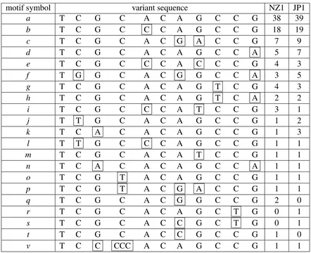
(29) motif x X. length 11 48. pattern TCGCACAGCCG TTCTGGGCAAAACGGCTGGGCGACGTGCTGGACTGGCCAGCTGGTTCG. Table 3.1: The consensus motifs x and X which form the nested tandem repeats in taro.. 3.1. Nested tandem repeat structures in NZ1 and JP1. The nested tandem repeats (NTRs) in NZ1 and JP1 show a substantial similarity which suggests that they are homologous. The NTRs in NZ1 and JP1 consist of two repeated motifs interspersed with one another. The two consensus motifs are listed in Table 3.1. In NZ1, there are 89 approximate copies of motif x and 12 approximate copies of motif X, whereas in JP1 there are 98 approximate copies of motif x and 13 approximate copies of motif X. Recall from section 1.2.3 that the structure of an NTR of the form xs0 Xxs1 X · · · Xxsn , may be presented in the form (s0 , s1 , . . . , sn ). Using this notation, the nested tandem repeat structures in NZ1 and JP1 are as follows: NZ1: (5,3,1,6,10,5,10,8,13,14,13,4) JP1: (4,3,1,6,7,8,4,10,12,10,16,13,4) The JP1 48 bp repeats are shown in Table 3.2.. 3.2. Nested tandem repeat variants sequence. There are 21 variants of the tandem motif in the NTRs in NZ1 and JP1, with the motif TCGCACAGCCG being the most frequent variant in each. These variants are listed in Table 3.3. These variants differ from each other by single nucleotide substitutions, apart from variant ‘v’ which is of length 13. The frequencies of the variants follow a power law (see Figure 3.1).. 3.3. Variants graph. As a result of mutational events that happened in the past, at the present time, we observe an NTR containing a set of variants. Each variant may have a frequency which is the number of its occurrences in the NTR. These frequencies depends on the rate of mutation (single nucleotide mutation), rate of duplication and rate of deletion (segment duplication 18.

(30) 19. 2 T T T T T T T T T T T T. 3 C C C C C C C C C C C C. 4 T T T T T T T T T T T T. 5 G G G G G G G G G G G G. 6 G G G G G G G G G G G G. 7 G G G G G G G G G G G G. 8 C C C C C C C C C C C C. 9 A A A A A A A A A A A A. 10 A A A A A A A A A A A A. 11 A A A A A A A A A A A A. 12 A A A A A C A A A A A A. 13 C C C C C A C A C A C A. 13a A. 14 G G G G G G G G G G G G. 15 G G G G G G G G G G G G. 16 T C C C C C C C C C C C. 17 T T T T T T T C T T T T. 18 G G G G G A G A G A G A. 19 G G G G G G G G G G G G. 20 G G G G G G G G G G G G. 21 C T C C C C C C C T C C. 22 G G G G G G G G G G G G. 23 A A A A A A A A A A A A. 24 C C C C C C C C C C C C. 25 G G G G G G G G G G G G. 26 T T T T T T T T T T T T. 27 G G G G G G G G G G G G. 28 C C C C C C C C C C C C. 29 T T T T T T T T T T T T. 30 G G G G G G G G G G G G. 31 G A G G G G G G G A G G. 32 A A A A A G A A A A A A. 33 C C C C C C C C C C C C. 34 T T T T T T T T T T T T. 35 G G G G G G G G G G G G. 36 G G G G G G G G G G G -. 37 C C C C C C C C C C C C. 38 C C C C C C C C C C C C. 39 A A A A A A A A A A A A. 40 G G G G G T G G G G G G. 41 C C C C C C C C C C C C. 42 C T T T T T T T T T T T. 43 A G G G G G G G G G G G. 44 T G G G G G G G G G G G. 45 T T T T T T T T T T T T. 46 T T T T T T T T T T T T. 47 C C C C C C C C C C C C. 48 G G G G G G G G A G G G. Table 3.2: The twelve 48bp motifs X in JP1 NTR in the order they appear in the NTR sequence. Substitutions are shown in boxes. Based on sites 13 and 18, the twelve strings are categorized into two motif families A or B. The last motif contains an insertion at position 13a and a gap at position 36.. A A A A A B A B A B A B. 1 T T T T T T T T T T T T.

(31) and deletion). We expect the frequencies of any two variants on average to be in the approximate ratio of 1:1 if the relative rate of mutation to duplication is high. On the other hand, if the relative rate of mutation to duplication is low we expect to have a small number of variants. The variants are hypothesised to be homologous (to have evolved from a single ancestral segment) with an ancestral history of duplication, substitution and deletion. If we knew this history, we could illustrate it by a tree T , rooted at the common ancestor, where each vertex represents a variant (historical or contemporary), and each edge represents a set of edit operations transforming an ancestor to its descendant. We use a parsimony principle for finding a tree T connecting the variants, where the total number of edit operations to transform the connected variants is minimal. When the variants are closely connected we consider the 1−cluster graph G1 = (V, E) motif symbol a b c d e f g h i j k l m n o p q r s t v. T T T T T T T T T T T T T T T T T T T T T. C C C C C G C C C T C T C C C C C C C C C. G G G G G G G G G G A G G A G G G G G G C. variant sequence C A C A C C C A C A C G C A C A C C C A C A C G C A C A C A C A C C C A C A C A C A C A C C C A C A C A C A C A T A C A T A C G C A C G C A C A C A C C C A C C CCC A C A. G G A G C G G G T G G G T G G A G G G G G. C C C C C C T T C C C C C C C C C C C C C. C C C C C C C C C C C C C C C C C T T C C. G G G A G A G A G G G G G A G G G G G G G. NZ1 38 18 7 5 4 3 4 2 3 1 1 1 1 1 1 1 2 0 0 1 1. JP1 39 19 9 7 3 5 3 2 1 2 3 1 1 1 1 1 0 1 1 0 1. Table 3.3: The 21 tandem motif variants of JP1 and NZ1. Each variant is assigned a character a, . . . , v. The frequency of each variant is listed in the third and fourth columns. Variants b to t comprise 11 bp, and differ from a by 1, 2 or 3 substitutions shown in boxes. Variant v comprises 13 bp with CCCCC replacing CGC in the 2, 3, and 4 sites. 20.

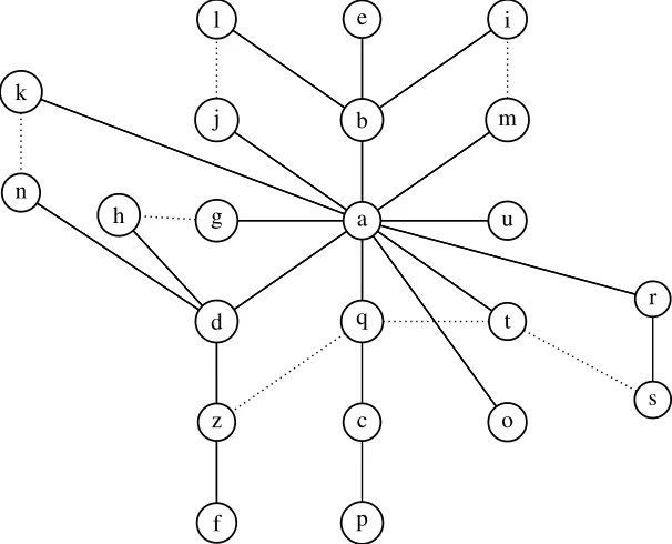
(32) 38 36 34 32 30 28 26 24 22 20 18 16 14 12 10 8 6 4 2 a. b. c. d. e. f. g. h. i. j. k. l. m n. o. p. q. s. t. Frequencies. Figure 3.1: Frequencies of all variants in NZ1. The ratios of the three most common variants a, b, and c appear to follow a power law. The frequencies of the variant a, b, and c are in the approximate ratio 4:2:1.. 21.

(33) (Hendy et al., 1980), where V is the set of contemporary variants and the set of edges E = {(u, v)|u, v ∈ V ; d(u, v) = 1} connects each pair of variants which differ by a single edit operation (single site substitutions and indels). However G1 will not usually be a tree. The graph G1 may contain circuits, for example, the four variants a, d, q, z in Figure 3.2. This may be the consequence of a parallel mutation, which can happen when the density of substitutions is high and the segments are short. l. e. i. j. b. m. g. a. u. d. q. t. z. c. o. f. p. k. n h. r. s. Figure 3.2: The variants graph of the taro variants with the template motif being TCGCACAGCCG, which is the variant a. The graph has two components, with variant f at distance 2 from its closest neighbours. An additional (unobserved) variant z is added to make the graph connected, which is not observed in the NTR region of JP1 and NZ1. Variant v=TCCCCCACAGCCG is not included. The set of edges in this graph is the union of the sets of edges of all minimum spanning trees. In each cycle in the graph, the edge that connect the two least frequent variants is drawn as a dashed line.. The set V may not contain all ancestral variants, as some may have been lost by deletion, and hence G1 might not be connected. This may occur if the substitution rate is higher than the duplication rate. Connectivity can be achieved by adding edges (u, v) with d(u, v) > 1, where u, v are in different components of G1 , and Steiner points (new vertices which could represent ancestral variants) when adjacent edges share some common edit operations, to reduce the total number of edit operations across the edges. For example, the variant f differs by more than one substitution from any other observed variant, and so we add the unobserved variant z (see Figure 3.2). 22.

(34) We will refer to a connected graph G which connects all the variants, and which may include additional hypothetical variants, and in which every edge represents an edit operation, as a variants graph. The construction of the variants graph is NP-hard (Foulds and Graham, 1982). The variants distance graph is the weighted complete graph with vertex set the set of variants, in which the edge between variants u and v is given weight d(u, v).. 3.4. Expected number of parallel substitutions. Single point substitutions happen in the duplication history of tandem repeats. These single substitutions produce a set of variants that we observe at the current time. The number of substitutions that occurred in the past is unknown, but a lower bound on the number of substitutions is the length of the Steiner tree of the variants, which can be approximated by the length of the minimum spanning tree of the distance graph. Note that the length of the Steiner tree is equal to the length of the minimum spanning tree when the variants graph is an 1−cluster (Hendy et al., 1980). However, some parallel substitutions may have occurred during the evolution of the nested tandem repeat, whereby an existing variant is created again. In this section, we calculate the likelihood P (k, i) that i observed substitutions are the result of k ≥ i substitutions on a motif of size n. There are 3n possible substitutions, where n is the length of the motif. A substitution can either be a new substitution or it can be parallel (it duplicates an existing substitution); in the second case the number of substitutions does not increase. If we observe i substitutions after k substitutions have occurred, then the (k + 1)−th substitution produces either a new substitution (with probability. 3n−(i−1) ), 3n. probability. i ). 3n. or reproduces an existing substitution (a parallel substitution with. Thus the probability P (k, i) of observing i substitutions after k > 0. substitutions can be calculated using the recursive formula. P (k, i) = P (k − 1, i − 1) ×. i 3n − (i − 1) + P (k − 1, i) × , 3n 3n. for k > 0, i > 0, 23.

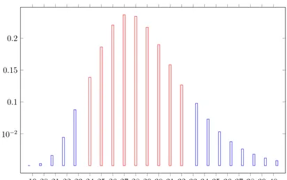
(35) 0.2. 0.15. 0.1. 5 · 10−2. 19 20 21 22 23 24 25 26 27 28 29 30 31 32 33 34 35 36 37 38 39 40 P (k, 19). Figure 3.3: The likelihood distribution of the number of substitutions to produce 19 variants of a motif of length 11 bp. Bars representing likelihood values greater than 0.1 are coloured in red. with initial values P (0, 1) = 1, P (0, i) = 0, P (k, 0) = 0 for i 6= 1. Figure 3.3 plots P (k, i) for n = 11 and i = 19, as is the case for the tandem motifs in NZ1. This suggests that the number of parallel substitutions in NZ1 is more likely to be in the range 24 − 19 = 5 to 32 − 19 = 13.. 3.5. Variants frequency distribution. Nested tandem repeat copies contain variants observed in different frequencies. For example, in NZ1, variant ‘a’ is observed 38 times, while variant ‘b’ is observed 18 times. The 2:1 distributions in Figure 3.1 suggests an early distribution is ‘aab’, ‘aba’ or ‘baa’. Ten possible duplication history scenarios that lead to a segment that consists of two ‘a’s and one ‘b’ are shown in Figure 3.4. There are eight minimal paths to generate ‘aab’, ‘aba’, or ‘baa’ from ‘a’, and two to 24.

(36) a. b. a. b. a. aa. bb. aa. bb. aa. ab aaa. ba aaa. aab. aaa baa. aba. Figure 3.4: Duplication history scenarios. The dashed lines represent substitutions and the solid lines represent duplications. There are 10 possible minimal paths to produce a segment of three characters that consists of two ‘a’s and one ‘b’ from a single segment ‘a’ (8 paths) or ‘b’ (2 paths). Note that there are two ways to obtain ‘aaa’ from ‘aa’, because we may duplicate either the first or the second character. generate them from ‘b’. Therefore, we will choose ‘a’ as the more likely ancestral variant. We assume that the duplication mechanism has no preference on which variant to copy. Therefore, the ratio of frequencies for the more frequent variants are expected to remain similar through the later stages of the duplication history. Variants occurring with low frequencies and close to each other in the sequence suggest they are recent.. 3.6. Variants spread. The distribution of variants in a repeated region is correlated with the time at which the variants were introduced. The earlier variants in the evolution of the NTR have a greater opportunity to be duplicated and therefore are likely to have both a greater spread in the sequence and a greater frequency. The spread here refers to the difference between the right most copy position and the left most copy position for a particular variant. A later variant must have a restricted spread unless there has been one or more parallel substitutions to independently produce additional copies. In Table 3.2 the variant ‘a’ occurs 38 times in NZ1 and 39 times in JP1 and is spread all over the NTR sequence, which leads to the conclusion that ‘a’ is the oldest variant and probably the ancestral variant. The frequency of variant ‘b’ is 18 which suggests it is more likely that the change from ‘a’ to ‘b’ happened in an early stage of the duplication history tree. Figure 3.3 suggests that the total number of substitutions is likely to be in the range 24 to 32, and so the number of parallel substitutions is likely to be in the range 5 = 24 − 19 25.

(37) to 13 = 32 − 19. If such a parallel substitution occurs in widely separated variant copies, then these variants will have a larger spread to frequency ratio. In Figure 3.6, we note that variants h, q, g, f have larger spread to frequency ratio. This suggests that it is more likely that these variants copies were a result of parallel substitutions. It is important to take the information on the spread of the variants into account when inferring the duplication history. a. 40. 20. Frequency. 30. 15 b. 20 10 i he. d q. g f. 10. c. 5. 0. 0 0. 20. 40 60 Spread. 80. i a b e h d c g f q Figure 3.6: Variant spread to frequency ratio. The variants c, g, f , and q have higher spread to frequency ratios, suggesting that they are likely to be the result of parallel substitutions.. Figure 3.5: Variant frequency plotted against spread. The spread refers to the difference between the positions of the right most and left most copies.. 26.

(38) Chapter 4 NTRFinder: A Software Tool to Find Nested Tandem Repeats This chapter reproduces the text of NTRFinder: a software tool to find nested tandem repeats, A. Matroud, C. Tuffley, and M. Hendy, Nucleic Acids Research (Matroud et al., 2012b). It has been reformatted for consistency with the rest of thesis, and some background and definitions have been moved to Chapter 1.. 4.1. Abstract. We introduce the software tool NTRFinder to search for a complex repetitive structure in DNA we call a nested tandem repeat (NTR). An NTR is a recurrence of two or more distinct tandem motifs interspersed with each other. We propose that nested tandem repeats can be used as phylogenetic and population markers. We have tested our algorithm on both real and simulated data, and present some real nested tandem repeats of interest. NTRFinder can be downloaded from http://www.maths.otago.ac.nz/ ˜aamatroud/.. 4.2. Introduction. Genomic DNA has long been known to contain tandem repeats: repetitive structures in which many approximate copies of a common segment (the motif ) appear consecu27.

(39) tively. Several studies have proposed different mechanisms for the occurrence of tandem repeats (Weitzmann et al., 1997; Wells, 1996), but their biological role is not well understood. Recently we have observed a more complex repetitive structure in the ribosomal DNA of Colocasia esculenta (taro), consisting of multiple approximate copies of two distinct motifs interspersed with one another. We call such structures nested tandem repeats (NTRs), and the problem of finding them in sequence data is the focus of this paper. Our motivation is their potential use for studying populations: for example, a preliminary analysis suggests that changes in the NTR in taro have been occurring on a 1,000 year time scale, so a greater understanding of this NTR offers the potential to date the early agriculture of this ancient staple food crop. The problem of locating tandem repeats is well known, as their implication for neurological disorders (Verkerk et al., 1993; Fu et al., 1992), and their use to infer evolutionary histories has urged some researchers to develop tools to find them. This has resulted in a number of software tools, each of which has its own strengths and limitations. Most of these software tools use statistical criteria on the distances between k-tuple matches (these distances are generally multiples n·` of the pattern length ` , where n ∈ {1, 2, . . . }). However, the distances between matching k-tuples in NTRs are of the form a · α + b · β, where α and β are the lengths of the two patterns and a, b ∈ {1, 2, . . . }. Consequently these software tools do not generally find NTRs. In this paper we present a new software tool, NTRFinder, which is designed to find these more complex repetitive structures. We report here the algorithm on which NTRFinder is based and report some of the NTRs it has identified, including an even more complex structure where copies of four distinct motifs are interspersed.. 4.3. Material and Methods. In this section we present the algorithm we have developed to search for nested tandem repeats in a DNA sequence. The algorithm requires several preset parameters. These are: k1 and k2 which bound the edit distances from the tandem and interspersed motifs; and the motif length bounds mint1 , maxt1 , mint2 , maxt2 . Other input parameters are discussed below. 28.

(40) Search phase. Our search is confined to seeking NTRs with motifs of length l1 ∈. [mint1 , maxt1 ] and l2 ∈ [mint2 , maxt2 ]. A (k1 , k2 )−NTR must contain a k1 −TR, so we begin by scanning the sequence for approximate tandem repeats. To do this we have chosen to adapt the tandem repeat search algorithm ATRHunter of Wexler et al., in which the sequence is searched for tandem motifs of length l1 by scanning the sequence with two windows w1 and w2 of width w, at distance l1 apart. This may be adapted to find nonadjacent copies of the tandem motif (as occur in NTRs) by holding w1 fixed, and moving w2 further away. The user may set the k1 , k2 values, preset with default values p k1 = l1 (1 − pm ) + l1 (1 − pm )pm p k2 = l2 (1 − pm ) + l2 (1 − pm )pm ,. (4.1) (4.2). following Domaniç and Preparata (2007), with matching probability pm given the default value pm = 0.8. Once a TR has been found and its full extent determined, the right-most copy of the repeated pattern is taken as the current TR motif x, and further approximate copies of x are sought, displaced from the TR up to a distance of maxt2 nucleotides to the right. This is done by moving the second scanning window w2 to the right, while holding the first fixed in the current copy of x. If no further approximate copies of x are located, this TR is abandoned, and the TR search continues to the right. If a displaced approximate copy of x is observed, then both x and the interspersed segment X are recorded in a list, as we have found a candidate NTR. Further contiguous copies of x are then sought, with the rightmost copy x replacing the previous template motif. The steps above are repeated with successive motifs x and interspersed segments copied to the list, until no additional copies of the last recorded motif x are found. This search phase is illustrated in Figure 4.1. At this point the algorithm builds consensus patterns for x and X using majority rule. After constructing the two consensus patterns the algorithm moves to the verification phase. 29.

(41) Example: An example will help illustrate the procedure. Suppose that S contains an NTR of the form xX0 xxxX1 xxxxxxX2 xxX3 . The algorithm will scan from the left until it locates the tandem repeat consisting of three copies of x between X0 and X1 . It will then start searching for additional non-adjacent copies of x to the right, locating the first copy to the right of X1 . Having found this it will record the intervening segment X1 , and then continue the tandem repeat search from this point until the full extent of the tandem repeat between X1 and X2 is found. This procedure is repeated once more, locating the tandem repeat between X2 and X3 , recording the segment X2 , and then searching for further copies to the right. At this point no more copies of x are found, and the process of verification begins. The segments X0 , X3 and the initial copy of x are found during this stage.. Verification phase:. Each candidate NTR is checked to determine whether it meets the. NTR definition. This is accomplished by aligning the candidate NTR region, together with a margin on either side of it, against the consensus motifs x and X, using the nested wrap-around dynamic programming algorithm of Matroud et al. (2011), presented in Chapter 5 of this thesis. The nested wrap-around dynamic programming parameters are set to be 2 for a match, −5 for a mismatch, and −7 for a gap. These parameters were chosen following (Wexler et al., 2005). The nested wrap-around dynamic programming algorithm has complexity O(n|x||X|), where n is the length of the NTR region and |x| and |X| are the length of the tandem motif and the length of the interspersed motif respectively.. A remark on tandem repeat detection, and the role of verification. The definition. of a k-TR requires that each repeat be a distance at most k from some template motif. However, this template is unknown during the search phase. We follow ATRHunter’s algorithm to compare each repeat copy with its preceding copy. Comparisons between adjacent copies will not miss any tandem repeats, provided the distance threshold is set appropriately, but may result in false positives due to “drift”. Such false positives are eliminated during the verification phase, when the candidate tandem repeat is aligned against the consensus motif. 30.

(42) Suppose that x1 x2 · · · xn is a k-TR with motif x. Then since d(x, xi ) ≤ k we have d(xi , xj ) ≤ d(xi , x) + d(x, xj ) ≤ 2k, by the triangle inequality. It follows that a tandem repeat search that correctly detects when d(xi , xi+1 ) ≤ d will find all (d/2)-TRs. We note however that a segment x1 x2 · · · xn satisfying d(xi , xi+1 ) ≤ d for all i need not be a tandem repeat, since xj may “drift” away from xi as j increases. A simple example is aaaa aaac aacc accc cccc, in which adjacent copies are distance 1 apart, but the first and last copies are distance 4 apart.. 4.4. Results. 4.4.1. Tests on simulated data. In order to measure the accuracy of NTRFinder, we generated synthetic sequence data containing NTR subsequences with varying probabilities of substitution and insertion and deletion (indels), and determined the proportion of the NTRs that were found by NTRFinder. In our simulation we first generated one random DNA sequence of 100000 nucleotides, with each nucleotide occurring with probability 0.25. Within this sequence we embedded 100 exact NTRs with repeats of randomly generated motifs X and x of varying lengths. From this sequence we generated four additional sequences by introducing indels and substitutions. Indels were introduced to each sequence with a constant probability of 1% per site, and substitutions were introduced with varying probabilities of 1%, 2%, 3% and 4% per site. NTRFinder recovered 95%, 84%, 83%, 83% and 80% of the NTRs respectively. These results are plotted in Figure 4.2. No false positives were detected. The first phase of NTRFinder uses a modification of the algorithm ATRHunter presented by Wexler et al. (2005). Wexler et al. report that ATRHunter has a 74%–90% success rate for finding ATRs in synthetic sequences, with average score of an ATR over all sequences being 238 with a standard deviation 116. These results suggest the accuracy 31.

(43) of the Wexler algorithm provides the major limitation on the accuracy of NTRFinder.. 4.4.2. Tests on real sequence data. To test NTRFinder on real sequence data we searched all intergenic spacer (IGS) sequences available in Genbank. The IGS sequences were chosen because we already knew of an NTR in the IGS region of C. esculenta. We also searched the entire Human Y chromosome from (Fujita et al., 2010). The size ranges used for this search were [mint1 , maxt1 ] = [mint2 , maxt2 ] = [2, 100], with the parameters k1 and k2 set to their default values given in equations (4.1) and (4.2) on page 29. NTRs found in IGS sequences are listed in Table 4.1. We searched 27 IGS sequences and found NTRs in 12 of them. NTRs found in the Human Y chromosome are listed in Table 4.2. The 11 NTRs found in the Y chromosome all appear to be in the psuedoautosomal region.. 4.4.3. More complex structures. In addition to the nested tandem repeats in Table 4.2, NTRFinder also reported an NTR in Linum usitatissimum (accession number gi| 164684852 | gb|EU307117.1|) which on further analysis by hand turned out to have a more complex structure. The IGS region of the rDNA of this species contains an NTR with four motifs interspersed with each other. The four motifs are w=GTGCGAAAAT, x=GCGCGCCAGGG, y=GCACCCATAT, and z=GCGATTTTG, and the structure of the NTR has the form 25 Y. wqi xri zsi yti ,. i=1. where qi ∈ {1, 2, 3}; ri ∈ {1, 2}; si ∈ {0, 1}; ti ∈ {0, 1}.. 4.4.4. Running time. The running time for NTRFinder searching some sequences from GenBank is shown in Figure 4.3. It can be seen that the run time is approximately linear in the length of the sequence. However, it must be noted that the run time depends not only on the length of the input sequence, but also on the number of tandem and nested tandem repeats found in 32.

(44) the sequence. The program spends most of the time verifying any tandem repeats found.. 4.5. Discussion. In the last decade a number of software tools to find tandem repeats have been introduced; however, little work exists on more complex repetitive structures such as nested tandem repeats. The problem of finding nested tandem repeats is addressed in this study. The motivation for our study is the potential use of NTRs as a marker for genetic studies of populations and of species. We have done some analysis on the nested tandem repeat in the intergenic spacer region in C. esculenta (taro), noting some variation in the NTRs derived from domesticated varieties sourced from New Zealand, Australia and Japan. Further varieties are currently being analysed.. 4.6. Conclusion. The nested tandem repeat structure is a complex structure that requires further analysis and study. The number of copy variants in the NTR region and the relationships between these copies might suggest a tandem repeat generation mechanism. In this paper, we have introduced a new algorithm to find nested tandem repeats. The first phase of the algorithm has O(n(maxt1 )(maxt2 )) time complexity, while the second phase (the alignment) needs O(n(maxt1 )(maxt2 )) space and time, where n is the length of the NTR region, and maxt1 , maxt2 are the maximum allowed lengths of the tandem and interspersed motifs.. 33.

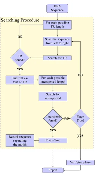
(45) DNA Sequence. Searching Procedure. no. TR found?. For each possible TR length. Scan the sequence from left to right. Search for TR. yes Find full extent of TR. For each possible interspersed length. no. Search for interspersed. Interspersed found?. no. Flag= True?. yes Record sequence separating the motifs. yes Flag:=True. Verifying phase Report. Figure 4.1: Flowchart of the NTRFinder algorithm.. 34.

(46) Percent of NTRs recovered (%). 100 80 60 40 20 0 0. 1 2 3 4 Substitution probability (%). Figure 4.2: Percentage of NTRs found in the synthetic sequences.. Species Accession number Nicotiana sylvestris X76056.1 Brassica juncea X73032.1 Brassica olerecea X56978.1 Brassica olerecea X60324.1 Brassica rapa S78172.1 Brassica campestris X73031.1 Colocasia esculenta Not published Nicotiana tomentosiformis Y08427.1 Arabidopsis thaliana CP002685.1 Zea mays AJ309824.2 Olea europaea AJ865373.1 Herdmania momus X53538.1. NTR structure (s0 , s1 , ..., sn ) (0,1,2,3,4,2,3,2,3,3,3,5,4,3,2,3,3,1,2,5,3,5,4,2,2,4,3) (9,12,2,6,2,5,4,1) (1,1,1,3,3,1,3,2,1,1,2,1,3,1,1,2,1,2,1,1,2) (1,1,1,3,3,1,3,1,3,2,1,1,2,1,3,1,1,2,1,2,1,1,2) (1,2,2,3,3,2,2,2,3) ( 6,4,4,7,4,4,4,3,1) (5,3,1,6,10,5,10,9,13,14,15,4) ( 1,1,2,2,1,2,4,2,1) (3,2,1,1) (2,2,1) (3,1,3,6,5,6,4,3,4) (3,1,1,1,1,0). |x| |X| 10 13 21 30 30 44 30 44 12 45 21 51 11 48 20 46 13 17 19 52 75 11 107 91. start index end index 960 2,111 1,403 2,605 1,031 2,902 1,036 3,133 385 1,337 1,558 2,580 725 2,384 1,016 1,969 32,189 32,365 2,984 3,113 961 3,743 6,363 7,642. Table 4.1: Nested tandem repeats found in some IGS sequences searched from GenBank and an additional unpublished sequence (C. esculenta).. 35.

(47) NTR structure (s0 , s1 , ..., sn ) (1,2,2,1,2,1,2,1,1,2,2,2,2,1) (7,22,23,12,14,4) (1,1,2,1,1,1,1,,1,1,1,1,1,1,1,1,1,1,1,1) (1,1,1,2,1,1,1,1,1,1,1,1,1,2,1,1,1,1, 1,1,1,1,1,1,1,1,1,1,1,1,1) (17,15,31,28,72,62) (3,6,8,11,7,6,4,4,5,4,11) (26,27,25,25,25,20,17,13,26) (1,2,1,2,1,2,2,2,2,2,1,2,1,1,1,2,2,2,1,2,2,1,1) (1,1,2,6,2,2,2,1,2) (1,1,1,0,2,1) (2,2,2,1,2,1,1,1,1,2,6). |x| |X| 12 56 2 88 15 14 11 16 2 49 12 32 1 48 16 22 19 35 19 56 21 15. start index end index 143,865 144,880 234,183 234,767 465,369 466,397 647,659 649,721 901,237 902,037 1,279,754 1,280,875 1,397,128 1,397,735 1,516,157 1,517,560 1,626,578 1,627,258 2,102,194 2,102,594 2,164,541 2,165,091. Table 4.2: Nested tandem repeats found in the Human Y chromosome (accession number NC 000024).. 36.

(48) Time (s). 102. 101. 100 104 105 Sequence length (bp). 106. Figure 4.3: Running time of NTRFinder (on a Pentium Dual core T4300 2.1 GHz) plotted against segment length on a log-log scale. The search was performed on segments of different lengths, with the minimum and maximum tandem repeat lengths set to 8 and 50 respectively. The distribution suggests the running time is approximately linear with sequence length.. 37.

(49) 38.

(50) Chapter 5 An algorithm to solve the motif alignment problem for approximate nested tandem repeats in biological sequences This chapter reproduces the text of An algorithm to solve the motif alignment problem for approximate nested tandem repeats in biological sequences, A. Matroud, C. Tuffley, and M. Hendy, Journal of Computational Biology (Matroud et al., 2011). It has been reformatted for consistency with the rest of thesis.. 5.1. Abstract. An approximate nested tandem repeat (NTR) in a string T is a complex repetitive structure consisting of many approximate copies of two substrings x and X (“motifs”) interspersed with one another. NTRs have been found in real DNA sequences and are expected to be important in evolutionary biology, both in understanding evolution of the ribosomal DNA (where NTRs can occur), and as a potential marker in population genetic and phylogenetic studies. This chapter describes an alignment algorithm for the verification phase of the software tool NTRFinder developed for database searches for NTRs. When the search algorithm has located a subsequence containing a possible NTR, with motifs X and x, a verification step aligns this subsequence against an exact NTR built from the 39.

(51) templates X and x, to determine whether the subsequence contains an approximate NTR and its extent. This chapter describes an algorithm to solve this alignment problem in O(|T|(|X| + |x|)) space and time. The algorithm is based on the wrap-around dynamic programming of Fischetti et al. (1993).. 5.2. Introduction. An approximate nested tandem repeat (NTR) in a string T is a complex repetitive structure consisting of many approximate copies of two substrings x and X (“motifs”) interspersed with one another. The name derives from the fact that an NTR may be thought of as two tandem repeats nested within one another. Approximate nested tandem repeats have been found in real DNA sequences, such as that of Colocasia esculenta, the ancient staple food crop taro (Matroud et al., 2012b). The intergenic spacer (IGS) region in the taro ribosomal DNA contains an NTR consisting of eleven approximate copies of a 48 bp motif, interspersed within a tandem repeat consisting of 96 approximate copies of an 11 bp motif. The NTR found in taro, used as a genetic marker, offers the potential to elucidate the prehistory of the early agriculture of this ancient food crop, as mutation events appear to be accumulating on a thousand-year time scale. NTRs in general also offer an opportunity to investigate concerted evolution whereby mutations are propagated throughout the many hundreds of copies of the IGS region in the taro genome. To develop a fuller understanding of the nature of NTRs, we have developed software to find them (Matroud et al., 2012b). This comprises two phases. The first phase is the detection phase, where the sequence is scanned to locate candidate NTRs and construct their consensus motifs X and x. The second phase is the verification phase where a subsequence containing a possible NTR, with motifs X and x, is aligned against all patterns of the form xs0 Xt0 xs1 Xt1 · · · xsk Xtk . Such an alignment is needed to find the extent and structure of the NTR (that is, to find the exponents si , ti occurring above), and may also be used to evaluate the fit of the template motifs x and X. We call this problem the motif alignment problem for NTRs, to distinguish it from the mapping problem (variants alignment problem) that arises at later 40.

(52) stages of the analysis. The purpose of this chapter is to present an algorithm to solve the motif alignment problem for approximate NTRs, given a sequence T, and the motifs x and X identified by our NTR search algorithm NTRFinder (Matroud et al., 2012b). Our alignment algorithm runs in O(|T|(|x| + |X|)) space and time, and plays a key rule in the verification phase of NTRFinder. It is based on the wrap-around dynamic programming technique introduced by (Fischetti et al., 1993) to solve the corresponding problem for (ordinary) tandem repeats. We show it can be readily adapted for use with more complex repetitive structures built from three or more motifs.. 5.3 5.3.1. Definitions Alphabets and strings. An alphabet is a nonempty set Σ of symbols or characters, and a string over Σ is a finite sequence of elements of Σ. We write Σ∗ for the set of all strings over the alphabet Σ, and |S| for the length of the string S. Given a string S and integers i, j such that 0 < i ≤ j ≤ |S|, we will write S[i] for the ith character of S, and S[i, j] for the substring consisting of the ith to jth characters of S. Given a second string T, the concatenation of S and T is the string ST, where. (ST)[i] =.   S[i]. if i ≤ |S|,.  T[i − |S|] if i > |S|. In applications to DNA sequences Σ is typically the set {A, G, C, T}, and we will use this alphabet in examples. However, our algorithm is not restricted to this case.. 5.3.2. The edit distance. In order to compare two strings X and Y it is useful to have some measure of the extent to which they differ. For the purposes of this chapter we will use the edit distance, where the edit operations we permit are the insertion of a single character; the substitution of a single character; or the deletion of a single character. 41.

No results found