Rochester Institute of Technology
RIT Scholar Works
Theses Thesis/Dissertation Collections
5-12-2017
Symbol Synchronization Techniques in Digital
Communications
Mohammed Al-Hamiri [email protected]
Follow this and additional works at:http://scholarworks.rit.edu/theses
This Thesis is brought to you for free and open access by the Thesis/Dissertation Collections at RIT Scholar Works. It has been accepted for inclusion in Theses by an authorized administrator of RIT Scholar Works. For more information, please [email protected].
Recommended Citation
R·I·T
Symbol Synchronization Techniques in Digital
Communications
by
Mohammed AlHamiri
A Thesis Submitted in Partial Fulfillment of the
Requirements for the Degree of Master of Science in
Telecommunications Engineering Technology
Electrical, Computer and Telecommunications Engineering
Technology
College of Applied Science and Technology
Rochester Institute of Technology
Rochester, NY
Committee Approval
___________________________________________________________________
Miguel Bazdresch Date
Thesis Advisor / Professor
___________________________________________________________________
William P. Johnson
Date
Committee Member / Professor
___________________________________________________________________
Steven Ciccarelli Date
Committee Member / Associate Professor
Abstract
Timing synchronization plays an important role in recovering the original transmitted signal in telecommunication systems. In order to have a communication system that operates at the correct time and in the correct order, it is necessary to synchronize to the transmitter’s symbol timing. Synchronization can be accomplished when the receiver clock tracks the periodic timing information in a transmitted signal to reproduce the original signal.
In this thesis work, we report the design, implementation and evaluation of a timing synchronization algorithm based on the technique first proposed by Gardner [1], applied to wireless communication using the Alamouti spacetime code [2] under QPSK modulation with halfsine pulses. To achieve this, a mathematical model is introduced which includes software design of communication algorithms. In this modeling, we simulate the Gardner algorithm in MATLAB. Then, five techniques are introduced to improve the performance of the loop filter in the digital receiver, and they are successfully implemented and evaluated in Matlab. These five techniques prove that there is an improvement in digital receiver performance in terms of the convergence speed and the communication system complexity.
we find them to be similar, proving that the synchronization algorithm is in fact achieving optimum synchronization.
This thesis presents synchronization algorithms that are necessary for a complete working wirelessAlamouti technique. Also, this thesis improves the communication system performance in terms of the convergence speed with reducing the computational complexity of the communication system design.
Table of Contents
1 Introduction ………... 08
1.1 Background ………..………. 08
1.2 Review of Past Studies and Deficiencies ……...…..………….……….….……..…...09
1.3 Purpose statement ………..………..……….………… 10
1.4 Hypotheses ………..………..……….……….. 11
2 Literature Review ………... 12
2.1 Quadrature Pulse Shift Keying (QPSK) ………...…....……….……….……. 12
2.2 Symbol synchronization ………...…...………..….………. 13
2.2.1 The problem of Timing Recovery ..…………...………..……….... 14
2.3 Timing Recovery Techniques ………..……….……… 16
2.3.1 Cluster Variance ………..……….. 18
2.3.2 Timing Recovery via DecisionDirected Methods ……..…….……… 19
2.3.3 Timing Recovery via Output Power Maximization …...…..……… 21
2.3.4 Gardner technique ………....…..……….……….…. 22
2.4 Alamouti spacetime code technique ………...………. 25
2.5 Gaps in the Literature ………..………. 29
2.6 Theoretical perspective ………...…..……… 30
3 Methodology ……….……….. 31
3.1 Research Design ……… 31
3.2 Elements of the experiment …………..………...…...………. 31
3.3.1 Dependent Variables ………..……… 32
3.3.2 Independent Variable ………..……… 32
3.4 Instrumentation and Materials ……….. 32
3.5 Procedure ………..…. 32
3.6 New techniques to improve the timing recovery in wireless receivers ………...…… 33
3.7 Baseline Matlab code of Gardner technique with BPSK ……….……… 34
3.8 The first technique to improve the timing recovery ………..….……….… 47
3.8.1 Evaluation of the first technique ………...……….……….. 56
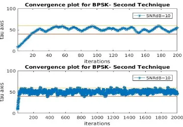
3.9 The second technique to improve the timing recovery …………...………. 56
3.9.1 Evaluation of the second technique ……….…..………...…… 61
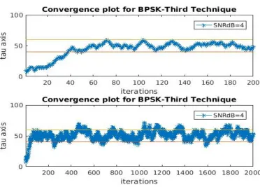
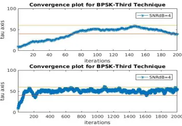
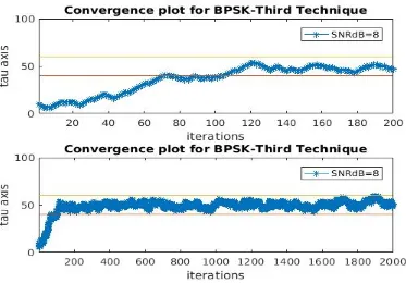
3.10 The third technique to improve the timing recovery (part #1) ….……….…….….. 61
3.10.1 Evaluation of the third technique (part #1) ……….……….. 66
3.11 The third technique to improve the timing recovery (part #2) …….……..………. 66
3.11.1 Evaluation of the third technique (part #2) ……….….…………. 70
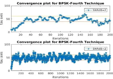
3.12 The fourth technique to improve the timing recovery ……….……….……… 71
3.12.1 Evaluation of the fourth technique ………..…...…….………….. 75
3.13 The fifth technique to improve the timing recovery ………...………….. 76
3.13.1 Evaluation of the fifth technique ……….……….…………...80
3.14 Summary and comparison of the five techniquesBPSK ………….…….………… 81
3.15 Baseline Matlab code of Gardner technique with QPSK ………….……….. 83
3.16 Summary and comparison of the five techniquesQPSK …………..…….….…….. 93
3.18 The third technique to improve the QPSKAlamouti Gardner (QAG) Tech….… 108 3.19 Summary and comparison of the five techniques that work with QPSK Alamouti
Gardner (QAG) Technique ……….……….…. 112
3.20 Limitations ……….………... 116
4 Conclusion and Future Research ……….. 117
4.1 Conclusion ……….…. 117
4.2 Future Research ……….. 118
Bibliography ………
119
Chapter 1
Introduction
1.1 Background
Synchronization is the process of technical coordination between transmitters and receivers in digital communication systems. Kihara, Ono, and Eskelinen [3] show that synchronization is required for fast and reliable data transfer from transmitters to receivers, and to enable every individual component to be synchronized wherever the component is placed in digital communication system. Transmitters and receivers must be mutually coordinated to transfer data successfully. The receiver accepts data as true information only when the receiver knows the digital clock of the transmitter, or when the receiver has the ability to regenerate the digital clock. So, it is impossible to have a communication system that properly works without using synchronization in communication devices [3].
According to the synchronization level, there are two types of digital communication systems: asynchronous and synchronous systems. In asynchronous systems, local clock synchronization is established; whereas, all clocks are completely bound together in synchronous systems. Kihara, Ono, and Eskelinen [3] state that, “Asynchronous clocks are assumed to be independent and no effort is made to force them to synchronism. Of course, here the clocks are synchronized in practice to some extent.”
symbol synchronization, and frame synchronization. The focus of this thesis is on the symbol synchronization. The term of symbol synchronization or the timing recovery has the same meaning in digital communication systems.
Figure 1.1: Receiver block diagram
1.2 Review of past studies and their limitations
In digital receivers, the timing recovery leads to obtain symbol synchronization. Floyd Gardner [1] states that timing adjustment can be achieved by interpolation if the sampling is not synchronized to the data symbols. Some of proposed solutions are to use synchronous Double Side Band systems. Costas [4] shows that Double Side Band has power advantage over Single Side Band when all factors, such as system complexity and susceptibility to jamming, are taken into account. Franks [5] illustrates that Maximumlikelihood estimation theory is another solution for the timing recovery which depends on root mean square jitter of the timing parameters as an approach to the evaluation of timing recovery circuit performance.
of the received signal can be maximized. This problem can be solved by a linear optimization technique such as gradient descent, which leads to a standard algorithm for timing recovery.
The previous studies focus on the synchronization techniques, but these studies ignored other important factors in designs of digital communication systems. In other words, these studies depend in their working on adding new components to the basic communication system. These components are added to detect the error in the synchronization process, such as error detection components, to manipulate the multipath fading, and to remove the noise that comes from external environment, such as filters. As a result, adding these components to the communication system leads to increase its complexities. These complexities can be described by the delay and the computational complexity that are produced by each additional component in wireless communication systems.
In terms of the delay, each component needs a time to conduct its required functions which is called the processing time. As a result, these additional components cause a delay for the wireless communication system. This delay has negative effects on the spectrum efficiency in term of the Bandwidth (BW). Also, this delay leads to decrease the speed of the convergence for the wireless communication system.
1.3 Purpose statement
that the QPSK modulation scheme has the ability to encode two bits per symbol which increases data rates and improves the spectrum efficiency.
In addition, the Alamouti technique [2] can be used to reduce the bit error rate by depending on the diversity improvements. The diversity technique has positive effects on the reception quality by reducing the fading effects. As a result, the Alamouti technique is used to reduce the required components to recover the original signal. Consequently, using QPSK modulation scheme with the Alamouti technique contribute in improving the performance of the digital communication system.
1.4 Hypotheses
This study aims to generate new algorithms and investigate if the new algorithms improve the digital communication system performance in term of the convergence speed with reducing the complexities of the communication system design.
H1: The new algorithms improve the digital communication system performance in term of the convergence speed with reducing the complexities of the communication system design.
H2: The new algorithms improve the digital communication system performance in term of the convergence speed without reducing the complexities of the communication system design
H3: The new algorithms improve the digital communication system performance by reducing the complexities of the communication system design without any improvement in the convergence speed.
H4: The new algorithms do not improve the digital communication system performance in term of the convergence speed and the complexities of the communication system design.
Chapter 2
Literature Review
This literature review introduces information about the QPSK modulation scheme, the symbol synchronization, timing recovery techniques, the Gardner technique, and the Alamouti spacetime code technique.
2.1 Quadrature Phase Shift Keying (QPSK)
QPSK is a digital modulation technique that sends two bits per symbol, and each symbol carries one of the four possible bit combinations (00, 01, 10, or 11). The phase of the carrier varies according to the symbol, and there are four phase shifts. The receiver needs to recover the original information from the modulated signal. QPSK is a bandwidth efficient because it sends two bits per symbol. That can be shown by comparison between QPSK and the Binary Phase Shift Keying (BPSK).
encoding rules that are used to represent the four possible phase shifts for QPSK modulation scheme.
The phase options The complex numbers
00 11j
01 1+1j
10 11j
[image:14.612.65.539.130.330.2]11 1+1j
Table 2.1: This table shows the encoding rules to represent the four phase options as complex numbers.
2.2 Symbol synchronization
The digital received signal passes through several components in the digital receiver which contribute to the recovery of the original transmitted signals [7]. One of these components is the digital demodulator, which is responsible for the acquisition of accurate symbol timing. Timing information that is obtained from synchronization is useful to delineate the digital received signal that is associated with a given symbol. Sampling techniques depend upon the timing information for amplitude, phase, and frequency demodulation [7].
The principle of timing synchronization depends on estimation of the timing offset 𝜏of the signal in AWGN channels. Digital wireless receivers face difficulties in estimating the value of 𝜏
most performance analysis of wireless communication systems it is assumed that the receiver synchronizes to the multipath component with delay equal to the average delay spread”. After this, the channel will be considered as AWGN to estimate the symbol timing.
In the symbol synchronization, the synchronizer takes samples for the received signal. As a result, these samples will be used to acquire symbols. Mueller and Muller [10] suggest timing algorithms that depend on just one sample per symbol and require directeddecision operations. In carrier system, correct decisions depend on carrier phase that should be known previously. As a result, this carrier phase will indicate the value of symbol timing which will result in increasing the system complexities.
Suzuki et al. [11] propose a different scheme which is called Wave Difference Method (WDM). This method “finds the average location of zeroslope of the received signal filtered signal pulses” [11]. Actually, this method requires numerous samples per symbol which may result in increasing the processing time. Therefore, this method increases the demand on the bandwidth (BW) which means decreasing the spectrum efficiency. Agazzi et al. [12] suggest using the previous method which is the Wave Difference Method with only two samples per symbol. This method works only with baseband signals which represent the demodulator output.
2.2.1 The problem of Timing Recovery
will be a function of the 𝜏 parameter [6]. This can be showed by the following formula which states the baseband waveform at the input of the sampler:
x( t )= ∑∞ s[ ] δ ( t T) ✳ g ( t ) ✳ c (t) ✳ g 🇷(t) + w (t)✳ g 🇷(t).
i= ∞ − i i т
where s[ ] represents the transmitted data, g ( t ) is the pulse shaping filter, c (t) is the i т impulse response of the channel, g 🇷(t) is the receiver filter, and w (t) is the noise. The three linear filters can be combined:
h(t)= g ( t ) c (t) g т ✳ ✳ 🇷(t) .
At ( kT/M + tau ) where M is the oversampling factor and T represents the interval between symbols, the sampled output can be written as:
x( kT/M + tau )= ∑∞ s[ ] h ( t T) + w (t)✳ g 🇷(t) .
i= ∞ − i i ∏
t=kT M +tau/
When the noise is supposed to have the same distribution whenever the samples are taken, the variance of the noise at the sampling time can be found without depending on the value of tau :
v(k)= w(t) g ✳ 🇷(t) ∏ .
t=kT M +tau/
By maximizing and minimizing some of the function of the samples, the value of tau can be found:
x(k) = x (kT/M + tau) = ∑ s[ ] h( KT/M + tau T) + v(k) . ∞
i= ∞ − i i
achieved by using an analog processor which determines when to sample. The third way can be accomplished by using a free running clock that chooses the sampling instants.
Figure 2.1: Three common structures for timing recovery. (a) Shows an analog processor. (b) States a digital post processor. (c) Use a free running clock and a digital post processor [6].
2.3 Timing Recovery Techniques
The problem of timing recovery is to find the features of performance functions at the optimal time. These performance functions are employed to indicate the adaptive elements which are responsible about estimation the sampling times [6, Ch. 12, pp. 226]. If the sampling times are incorrectly taken away from the optimal time, this will result in an error which is called the source recovery error. This source recovery error represents the error between the transmitted data and the received data. C. R. Johnson, Jr. and W. A. Sethares [6] state that the source recovery error can be calculated only when there is a training sequence or when the transmitted data are known.
Another way to estimate the error between the transmitted data and the received data is by using the cluster variance. The cluster variance suggests taking the square between the nearest element of the source alphabet and values of the received data [6]. The measurement of the power of the T spaced output of the matched filter is another approach to estimate the error. The estimation can be done by maximizing this output power which results in defining the adaptive element that is necessary to find the optimal time [6].
Figure 2.2: The effects of the transmitter pulse shaping g , the channel c, and the receive т filter g 🇷 can be represented by the transfer function h [6].
power method or the cluster variance method as a basis to find the optimal time [6]. The quality of the timing offset 𝜏 can be measured by using the cluster variance which is explained in the following section.
2.3.1 Cluster Variance
The decision device Q(x[k]) quantizes the binary data to the number that is closed to it [6]. In other words, the decision device converts any negative value to 1, and any positive value to +1. In the case of the timing offset is larger than T/2 and smaller than T/2, the eye is open, and the
Q(x[k]) =S[k1] for all k, and the source recovery error can be represented by:
e[k]=s[k1] – x[k]= Q(x[k]) x[k] .
If the timing offset is smaller than T/2 or larger than T/2, the Q(x[k]) will not be equal to
s[k1]. The Cluster Variance can be written as:
CV= avg{e 2 [k]}= avg{(Q(x[k]) – x[k]) 2 } .
Figure 2.3: Cluster variance as a function of timing offset 𝜏 [6].
C. R. Johnson, Jr. and W. A. Sethares [6] state that the previous measure is applied in the simple case. The simple case includes a channel without noise, the pulse shape h(t) is a triangle pulse, the transmission is binary data, and there is no inter symbol interference ISI. In this ideal situation, the timing offset 𝜏 can be indicated either by maximizing the output power or by minimizing the cluster variance [6]. There are two methods that can be used to design adaptive elements that are responsible about the maximization or the minimization.
2.3.2 Timing Recovery via DecisionDirected Methods
It is not possible to calculate the source recovery error i n the normal situation when there is no a training sequence. So, the timing recovery algorithm for the simple case cannot be applied in the normal situation. To solve this problem, C. R. Johnson, Jr. and W. A. Sethares [6] derived an algorithm to find the optimal value:
𝜏[k+1]= 𝜏[k] + µ(Q(x[k]) – x[k]) [x(kT/M + 𝜏[k] + δ) – x(kT/M + 𝜏[k] – δ)] .
where the µ is the step size. The step size can be reduced, or the numbers of the average values can be increased to eliminate the effect of the noise on the value of [k] . It is true that these two ways can reduce the influence of the noise, but they will slow the convergence of the algorithm. The algorithm above requires three samples for each symbol from the waveform, but it can be implemented easily. This can be done by taking samples three times straightforwardly [6]. The sampling is a hardware intensive solution because it involves hardware to achieve the sampling process.
The sampling theory states that any signal can be correctly reconstructed if it is sampled faster than twice the frequency. As a result, the value of the signal at x(kT/M + 𝜏 ) can be used to interpolate and find the value of the signal at x(kT/M + 𝜏[k] + δ) and at x(kT/M + 𝜏[k] – δ) [6] .
Figure 2.4: The adaptive element involves three interpolators. After the convergence of 𝜏[k], the
x[k] has the samples taken at times that minimize the cluster variance [6].
2.3.3 Timing Recovery via Output Power Maximization
The goal of timing recovery algorithm is to find the optimal time for sampling. This sampling can be done by maximizing the average of the received power (avg{x 2 [k]}). This
approach gives the same result that can be achieved by minimizing the cluster variance. This approach introduces an element that adapts 𝜏 to find the optimal time that maximizes the output power. C. R. Johnson, Jr. and W. A. Sethares [6] derived an algorithm to find the optimal value:
𝜏[k+1]= 𝜏[k] + µ x[k]) [x(kT/M + 𝜏[k] + δ) – x(kT/M + 𝜏[k] – δ)] .
The µ is the step size. If the µ is decreased, this can reduce the effect of the noise . Also, the effect of the noise can be eliminated by reducing the number of element that is used to find the average. However, this leads to reduce the speed of the convergent plot. This algorithm is a software intensive solution, and it can be showed by the next figure.
Figure 2.5: The adaptive element involves three interpolators. After the convergence of 𝜏[k], the
x[k] has the samples taken at times that maximize the output power [6].
The value of x(t) can be reconstructed at ( x(kT/M + 𝜏[k] + δ)]) and at x(kT/M + 𝜏[k] – δ)] from x[k]. This timing recovery algorithm can be implemented in digital, hybrid, and analog form [6].
As a result, these algorithms present solutions for the timing recovery which result from the mismatching between the receiver and transmitter clock. In addition to the timing recovery algorithms explained above that are suggested by C. R. Johnson, Jr. and W. A. Sethares [6] , there are other techniques that are usually used for timing recovery. These techniques are the Mueller and Muller technique, the earlylate technique, bandedge timing synchronization technique, and the Gardner technique.
2.3.4 Gardner technique
[13] demonstrate that this in turn increases the Bit Error Rate (BER) and decrease the Signal to Noise Ratio (SNR).
The following figure shows the block diagram of the receiving modem that is proposed by Gardner [1]. The received data is divided into two streams which are the Inphase stream and the Quadrature stream. Then, the two streams are demodulated to convert the passband data to baseband data by two of quadraturedriven mixers. The carrier recovery branch is omitted from the block diagram because it is not related to the timing recovery algorithm. After the mixers, two data filters are used to avoid unwanted mixers products, remove the noise, and to shape the received data.
Figure 2.6: Typical modem (block diagram of Gardner) [1]
time, and the other one occurs midway between the data strobe times”. Also, samples in these two sequences are transmitted, spaced by time interval T. The following error detector algorithm that is introduced by Gardner [1] can be showed by:
Ut(r)=yı(r½)[yı(r)yı(r1)] + y🇶(r½)[y🇶(r)y🇶(r1)] .
where r is the index that is used to designate the symbol number. The algorithm contains two parts, Inphase and Quadrature. In the Inphase part, the yı(r½) is midway sample between the yı(r) sample and yı(r1) sample . In the Quadrature part, the y 🇶(r½) is midway sample between the y 🇶(r) sample and y 🇶(r1) sample. The detector depends on the samples to find one error sample Ut(r) for each symbol. The loop filter is used to smooth the error sequence, and then this error sequence is used to adjust a time error corrector.
Gardner’s paper [1] concerns about the error detector, and it does not treat the loop filter or the error corrector. Gardner [1] proves that his algorithm (the Gardner algorithm) is independent of carrier phase. If Binary Phase Shift Keying (BPSK) modulation scheme is used in the communication system and in I channel, then the first part {yı( ) } of the above formula will be used to find the timing information. Of course, the {y 🇶( ) } will produce noise without any timing information. On the other hand, if Quadrature Phase Shift Keying (QPSK) modulation scheme is used in the communication system, then the both parts {yı( ) } and {y 🇶( ) } will be employed to find the timing information.
gives nonzero magnitude, and the magnitude of this midway sample depends on the timing error value [1]. When there is no transition, the values of the strobe samples should be the same, and the difference between them gives zero. This means that there is no timingerror information when there is no transition, and in this case the value of the midway sample rejects.
Gardner [1] suggests using just the sign of the strobe samples to recover the symbols instead of the actual values. This, in Gardner’s opinion, eliminates the noise effect if the data is filtering before taking the strobe samples. In this case, the signs of strobe samples are the optimum hard decision way to find symbols, and this makes the algorithm as a decision directed algorithm. This decision directed algorithm is similar to the digital transition tracking loop of Lindsey and Simon [14]. This thesis treats the loop filter and introduces five techniques to improve the communication system performance with taking into consideration the effect of the actual values of strobe samples.
2.4 Alamouti spacetime code technique
Alamouti [2, p.7] suggests using a technique to improve the diversity at all receivers in wireless systems. This can be achieved by using two transmitters and M receivers which will result in providing a diversity order of 2M. Consequently, this diversity improvement will positively affect Rayleigh fading. This technique does not require any feedback from the received antennas to transmitted antennas which is important for other techniques. Alamouti [2] shows that,”The scheme requires no bandwidth expansion, as redundancy is applied in space across multiple antennas, not in time or frequency.”
Also, Alamouti [2] proved that the assumed diversity scheme reduces the error rates, and increases the capacity of wireless communication systems. The Alamouti technique can be used by all applications that are limited by the Rayleigh fading. The diversity is usually improved by using a one transmitter and M receivers which result in providing a diversity order of M, and this is called receive diversity. However, the Alamouti provides transmit diversity by using two transmitter and M receivers which result in providing a diversity order of 2M
.
In this thesis, a flat fading Rayleigh multipath channel is applied. Quadrature Phase Shift Keying (QPSK) modulation scheme is used with two transmitted antennas and a one received antenna. This diversity scheme is called the Alamouti Space Time Block Coding (STBC), and it can be explained as follow:
1 Assume that the transmitted sequence is {X1, X2, X3, …, Xn} 2 The transmitted sequence groups into two groups.
3 In the first time slot, X1 and X2 are transmitted from the first and second antenna. In the second time slot, −X* and are transmitted from the first and second antenna. In the
2 X*1
third time slot, X3 and X4 are transmitted from the first and second antenna. In the fourth time slot, −X* and are transmitted from the first and second antenna and so on.
4 X3*
Figure 2.7: Alamouti scheme with two transmitted antenna and a one received antenna.
Time t Time t + T Antenna #1 x1 −x2* Antenna #2 x2 x1*
Table 2.2: The encoding and transmission sequence for the two branch transmit diversity scheme. 5 Although each channel is randomly varying, it is proposed that each channel remain constant over two time slots.
6 The noise on the received antenna in Gaussian distribution. 7 At the receive antenna, the channel is assumed to be known.hi 8 The received signal at the first time slot is:
= + + .
y1 h1 x1 h2 x2 n1 And in the second time slot is:
= + + .
y2 −h 1 x*
2 h2 x*1 n2
where
and are the received symbols on the first and second time slot,
y1 y2
and are the transmitted symbols,x1 x2
and are the noise in the first and second time slots respectively.
n1 n2
9 Then the above two signals go to the combiner that builds the following two signals
. y y
x︿1 = h*
1 1 + h2 *2
. y y
x︿2 = h*
2 1 −h1 *2
10 The above two signals are sent to the Maximum likelihood detector to find the final signal which compares with the original signal to find the Bit Error Rate (BER).
2.5 Gaps in the Literature
In the past studies, the researchers add new components to improve the quality of communication systems, but they ignored that these additional components increase the processing time in wireless communication systems. Also, the researchers use techniques that consume a part of the bandwidth as a feedback to synchronize between transmitters and receivers. Moreover, some researchers state that the bandwidth can be sacrificed or the power can be increased to manipulate the Rayleigh fading. Gardner [1] suggests using two samples per symbol for the timing recovery, but his technique consumes put burden on the bandwidth.
2.6 Theoretical perspective
This thesis depends on the estimation theory which provides the theoretical framework for studying the symbol timing problem. Also, this thesis presents ideas to improve the loop filter in the phase locked techniques depending on the Gardner technique. The Alamouti technique, in turn, improves the diversity order which reduces impacts of Rayleigh fading and increases the range of the coverage area. The previous studies state that the QPSK modulation scheme can be used to transmit high data rates. So, QPSK modulation scheme presents good solutions for increasing the demand on the bandwidth. As a result, this study will take advantage by using the Alamouti technique with timing synchronization technique that involves a new loop filter for QPSK modulation scheme.
Chapter 3
Methodology
3.1 Research Design
This research is a quantitative research because it involves an experimental design that can be accomplished by generating new algorithms by using Matlab. The results will state which one of the hypotheses will be realized. These results will also show conditions and requirements of wireless communication system. In other words, the simulation will present perspectives about the behavior of digital receivers with the new techniques in the wireless communication systems. Moreover, the techniques can be practically implemented in the future to demonstrate their limitations in wireless communication systems. Furthermore, the techniques, which are introduced to improve the performance of phase locked loops, take into consideration reducing the receiver complexities.
3.2 Elements of the experiment
Data streams, which are modulated by QPSK modulation scheme, will be used as input data for the wireless communication system. The procedure is a quasiexperiment because participants which are the data amount are not randomly assigned. In other words, there are several modulation schemes that can be used in this study such as Amplitude Modulation (AM), Frequency Modulation (FM), and Quadrature Amplitude Modulation (QAM), but only QPSK modulation scheme is used in this work.
3.3 Variables
3.3.1 Dependent Variables
The results of MATLAB are the dependent variables because these results depend on algorithms of symbol synchronization techniques. These results are represented by the Bit Error Rates (BER), the Signal to Noise Ratio (SNR), and convergence plots.
3.3.2 Independent Variable
The algorithms of symbol synchronization techniques are the independent variables because these algorithms affect the results of MATLAB. In other words, when these algorithms change, this means that the results also change.
3.4 Instrumentation and Materials
This thesis is a quantitative research that involves an experimental design. The instruments and materials that will be used in this study include:
● Synchronization algorithms.
● MATLAB program.
● Lab computer.
● Windows Operating System.
● Linux Operating System.
3.5 Procedure
communication system that involves a transmitter, an AWGN channel including Rayleigh fading, and a receiver. The number of filters and feedback loops in the wireless system are reduced as much as possible to decrease the processing time and reduce the complexities of the communication system. The modulation scheme is Quadrature Phase Shift Keying (QPSK), and the Alamouti technique is used as a diversity technique to eliminate the Rayleigh fading. Then, MATLAB program is run, and the results are appeared in plots. This allows assuring that symbol synchronization algorithms work properly and logically.
3.6 New techniques to improve the timing recovery in wireless receivers
In this section, five techniques are introduced to improve the timing recovery in wireless receivers. The main part in the wireless receiver is the Phase Locked Loop (PLL) which consists of three parts: the error detector, the loop filter, and the error corrector. The five techniques improve the performance of the timing recovery by depending on developing new algorithms for the loop filter. The error detector of the Gardner technique is used for the five techniques. The modulation schemes that are used are Binary Phase Shift Keying (BPSK) and Quadrature Phase Shift Keying (QPSK).
(MSE), SNR vs. BER behavior, and the level of complexities of the wireless receiver design that can result from each technique for both modulation schemes BPSK and QPSK.
3.7 Baseline Matlab code of the Gardner technique with BPSK
The first two sections in the code are the data generation and the pulse shape. The following code shows how the data amount is modulated:
________________________________________________________________________________ Baseline_GardnerBPSK.m: Data generation and the pulse shape.
________________________________________________________________________________
%% Data generation
N = 3*10^6; % Number of bits
ip = rand(1,N)>0.5; % Generating 0,1
data = 2*ip1; % BPSK modulation
Tsym = 100; % No. of samples per symbol
MSE = zeros(1,5); % A memory for the MSE
BER_sim = zeros(1,5); % A memory for the simulated BER %% Pulse shape
p = sin(2*pi*(0:Tsym1)/(2*Tsym)); % Sinusoidal wave
data_up = zeros(1,length(data)*Tsym); % Creation a memory of zeros
data_up(1:Tsym:end) = data; % Interpolation the data
w = conv(data_up,p); % The convolution operation
______________________________________________________________________
The BPSK modulation scheme is used to transmit 3 × 10⁶symbols. Tsym states that one hundred samples per symbol are used in this code to simulate the impact of the interpolator. Then, pulse shape is applied on the signal. Each symbol is represented by the half of a sinusoidal cycle (this pulse shape is usually called a “halfsine”) that has one hundred samples.
the detection and correction process starts at the receiver. This section starts with giving information about initial values.
According to the Gardner technique, the optimal value for midway samples should be at (n 100), where n is the sequence of symbol in data. The first midway sample (called center in × the code) is assumed to be received at 60. In addition to midway sample, the Gardner algorithm involves finding the “early sample” and the “late sample”. The early and late samples can be calculated by finding the value of samples at ( center+delta ) and ( centerdelta ). The value of delta is equal to the half symbol period which is equal to ( Tsym /2=50).
After applying the Gardner algorithm, the shift value, that is used to correct the sampling operation, depends on the finding the average of a few iterations of the algorithm. In this code, the number of iterations is assumed to be equal to six (called avgsamples in the code). The Gardner technique supposes that the correction depends on the sign of the average result more than the value itself [1], so the step size is assumed to be equal to 1. Actually, this section of code is the focus of this thesis, so the development and the improvement are applied on it. After the initial values are given, another inside loop is created to conduct the error detection, loop filter, and the correction operations.
samples can be used to recover the symbols of data. In this Matlab code, early samples are used to recover symbols of received signal. When the end of the received signal is reached, the loop ends.
Error detection is simulated by applying the subtraction process and the Gardner algorithm. Then, the loop filter is simulated by finding the mean of several instantaneous timing estimates. If the sign of the mean is positive, the tau value is equal to 1. Otherwise, the tau value is equal to 1. Next, the rest of the Matlab codes are completed. The remind step is used to state how fast the convergence happens. When the convergence happens, this means that samples are taken close or at the optimal value. In other words, the samples at these optimal times are less affected by the noise; consequently, there are fewer errors in the symbols’ detection process.
In order to use the original convergence plots in the comparison with convergence plots of the five techniques, the Mean Squared Error can be used in this comparison. According to [15], the Mean Squared Error (MSE) can be calculated by applying the following formula:
MSE = n1 ∑n
i=1 (Y i Y ) .
︿
− i 2 where n: the number of iterations.
: the estimated tau.Y︿i Y i: the optimal tau.
Then to find the MSE, values of tau are saved in a vector. Next for the correction, the value of tau is added to the current center plus the 100 that is necessary to move to the next symbol. The following code demonstrates the above sections:
_____________________________________________________________________________ Baseline_GardnerBPSK.m: Noise addition,detection and correction.
________________________________________________________________________________
%% Noise addition
SNRdB=2:2:10; % Signal to Noise Ratio
SNR=10.^(SNRdB/10); % The linear values for the noise
for cv=1:length(SNR) % Generate a loop
received=w+noise; % Received signal with noise
%% Detection and Correction
tau=0; %Initial value for tau
delta=Tsym/2; %The shifting value before and
%after the midway sample
center=60; %The assumed place for the first
%midway sample
a=zeros(1,N1); %A memory of zeros for the
%earlier samples
cenpoint=zeros(1,N1); %A memory of zeros for the
%midway samples
remind=zeros(1,N1); %A memory of zeros for the remind
avgsamples=6; %Six values of Gardner algorithm
%are used to find the average
stepsize=1; %Correction step size
rit=0; %Iteration counter
GA=zeros(1,avgsamples); %A memory of zeros
tauvector=zeros(1,1900); %A memory of zeros for tau
%vector(2000100=1900)
uor=0; %A counter for the tau vector
for ii= (Tsym/2)+1:Tsym:length(received)(Tsym/2)
rit=rit+1; %A counter
midsample=received(center); %The midway sample
latesample=received(center+delta);%The late sample
earlysample=received(centerdelta); %The early sample
a(rit)=earlysample; %Save samples
%% Error detection
sub=latesampleearlysample; %Subtraction process
GA(mod(rit,avgsamples)+1)=sub*midsample;
%Gardner Algorithm
%% Loop filter
if mean(GA) > 0
tau = stepsize; %Shift by decreasing
else
tau = stepsize; %Shift by increasing
end
%% Safe remind values
cenpoint(rit)=center; %Save positions of
%midway samples
remind(rit)=rem((centerTsym/2),Tsym);
%Save remind values to find
% convergence plots %% tau vector
%2000 where the convergence
uor=uor+1; %happens
tauvector(uor)= (remind(rit) (Tsym/2)).^2;
%Difference between the
%estimated tau & the
end %optimal tau %% Correction
center=center+Tsym+tau; %Adding the tau value
if center>=length(received)(Tsym/2)1
break; %Break the loop when
%the midway sample reaches
%to 51 samples before
%the last sample
end
end
________________________________________________________________
Now, it is necessary to state that the value of tau depends on error information which can be obtained when there is a transition between symbols. The next four scenarios shows how the
tau value is taken. Scenario #1
The first scenario supposes that there is a BPSK signal that contains just two bits [1, 1]. The following figure shows where the early, midway, and late samples are taken:
Figure 3.1: shows the early, midway, and late samples of the first scenario
A L )
G = M * ( −E
= .50 * (−0.5−0.5)= −0 .5
where GA is the Gardner algorithm. M is the midway sample. L is the late sample. E is the early sample.
The optimal midway samples should be taken at (n 100) where n is the sequence of the × symbol. The midway sample in figure 3.1 is before the optimal value, so it should be shifted forward by the step size . The Gardner [1] uses the sign of the mean of several instantaneous timing estimates and ignores the actual value of the mean in the correction operation. As a result, when the sign is minus, the tau should be 1.
Scenario #2
The second scenario supposes that there is a BPSK signal that also contains just two bits [1, 1]. The following figure shows where the early, midway, and late samples are taken:
Figure 3.2: shows the early, midway, and late samples of the second scenario
GA = −0 * (.5 −0.5−0.5)= 0.5
The optimal midway samples should be taken at (n 100). The midway sample in figure × 3.2 is after the optimal value, so it should be shifted backward by the step size . As a result, when the sign is positive, the tau should be 1.
Scenario #3
The third scenario supposes that there is a BPSK signal. This signal contains just two bits [1, 1]. By using the Gardner algorithm on the samples of figure 3.3, the result will be as below: GA = −0 * (.5 0.5−(−0.5))= −0 .5
The optimal midway samples should be taken at (n 100). The midway sample in figure × 3.3 is before the optimal value, so it should be shifted forward by the step size . As a result, when the sign is negative, the tau should be 1.
Figure 3.3: shows the early, midway, and late samples of the third scenario
Scenario #4
Figure 3.4: shows the early, midway, and late samples of the fourth scenario
By using the Gardner algorithm, the result will be as below: GA = .50 * (0.5−(−0.5)) = 0.5
The optimal midway samples should be taken at (n 100). The midway sample in figure × 3.4 is after the optimal value, so it should be shifted backward by the step size . As a result, when the sign is positive, the tau should be 1.
The above four scenarios states that tau should be 1 when the sign of the mean of several instantaneous timing estimates is minus. However, the tau should be 1 when the sign of the mean of several instantaneous timing estimates is positive.
computing the BER. The following code demonstrates MSE, convergence plot, and the BER calculation sections: ________________________________________________________________________________ Baseline_GardnerBPSK.m: MSE, convergence plot, and the BER calculation. ________________________________________________________________________________
%% Mean Squared Error (MSE)
MSE(cv)=mean(tauvector); %Finding the Mean Squared Error
%% convergence plot
figure
symbols = 200;
subplot(2,1,1);
plot(remind(1:symbols), '*' );
hold on
lim1=40*ones(1,symbols);
lim2=60*ones(1,symbols);
plot(lim1);
hold on
plot(lim2);
title( 'Convergence plot for BPSKGardner' );
ylabel( 'tau axis' ), xlabel( 'iterations' )
legend( [ 'SNRdB=' int2str(SNRdB(cv))]);
axis([1 symbols 0 Tsym]);
subplot(2,1,2);
symbols = 2000;
plot(remind(1:symbols), '*' );
hold on
plot(lim1);
hold on
plot(lim2);
title( 'Convergence plot for BPSKGardner' );
ylabel( 'tau axis' ), xlabel( 'iterations' )
legend( [ 'SNRdB=' int2str(SNRdB(cv))]);
axis([1 symbols 0 Tsym]);
%% Calculating the simulated BER
Error=0; %Set the initial value for Error
for k=1:N1 %Error calculation
if ((a(k)>0 && data(k)==1)||(a(k)< 0 && data(k)==1))
Error=Error+1;
end
end
BER_sim(cv)=Error/(N1); %Calculate error/bit
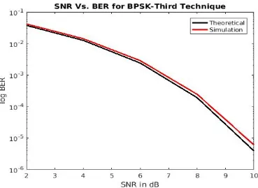
Finally, the theoretical BER is calculated as it is illustrated in the next code. Then, the SNR vs. BER figure is plotted as it is showed in the following code:
________________________________________________________________________________ Baseline_GardnerBPSK.m: SNR vs BER plot.
______________________________________________________________________
%% Plot SNR Vs BER
BER_th=(1/2)*erfc(sqrt(2*SNR)/sqrt(2)); %Calculate The
%theoretical BER
figure
semilogy(SNRdB,BER_th, 'k' , 'LineWidth' ,2); %Plot theoretical BER
hold on
semilogy(SNRdB,BER_sim, 'r' , 'LineWidth' ,2); %Plot simulated BER
title( 'SNR Vs. BER for BPSKGardner technique' ); legend( 'Theoretical' , 'Simulation' );
ylabel( 'log BER' ); xlabel( 'SNR in dB' );
_________________________________________________________________________________
The above Matlab codes represent the baseline codes of the Gardner algorithm. Note that the initial value for the midway sample is taken at 60, so the first early sample is taken at:
Figure 3.5: BPSKGardner technique, SNR= 2 dB
Figure 3.7: BPSKGardner technique, SNR= 6 dB
Figure 3.9: BPSKGardner technique, SNR=10 dB
Finally, the convergence plots can be used in the comparison operation with convergence plots of the five techniques. The following table states the values of MSE that are corresponding to the SNR values for the original convergence plots.
SNR 2 dB 4 dB 6 dB 8 dB 10 dB MSE 36.9274 28.8579 23.5400 18.2811 13.9632
Table 3.1: states SNR values with MSE value Gardner technique
3.8 The first technique to improve the timing recovery
This technique works on the error detection code and on the loop filter code. Otherwise, all other sections of the baseline Matlab code are used in this technique. This technique introduces a factor equal to 20 that can be multiplied by the result of error samples for the Gardner algorithm to give a faster correction operation. As it is mentioned before, this thesis assumes that there are one hundred samples per each symbol to simulate the effect of the interpolator. This means that there are one hundred magnitudes in each symbol. The maximum magnitude for the BPSK symbol is equal to 1 in the positive part, and the magnitude is equal to 1 in the negative part. In other words, the peak to peak magnitude for each symbol is equal to 2. As a result, there are one hundred different magnitudes in this range from 1 to 1. So, the difference in the magnitude between a one sample and the next sample is equal to 0.02. The following equation states that:
=
D =
V {p p}T sym− 1002= 0
.02
where
D: is the difference in the magnitude between one sample and the next sample.
is the magnitude from peak to peak which is equal to (2). {p }
Tsym : is the number of samples per symbol.
One of things in this technique that should be understood is that the value of D changes when the number of samples per symbol changes. To understand this technique, the following scenario introduces a good explanation that starts from the end to find the factor. This scenario supposes that the transmitted data are [1, 0], so this means that the BPSK is [1, 1]. After the pulse shape, the output is a sine wave signal. The following figure represents these two bits:
Figure 3.11: BPSK signal represents [1, 1]
At optimal time, the first midway sample should be received at sample#100, and its magnitude should be equal to zero when there is no noise. The earlier sample should be equal to (1) at sample#50, and the late sample should be equal to (1) at Sample# 150.
The following scenario#1 supposes that the first midway sample is received at 101. Theoretically, this means that the midway sample is one step away from the optimal position and in the negative part, and its magnitude is
Midway sample = Nu D .×
= 1 0.02= ×
−
0.02.
where
Nu : is the number of steps that is supposed to be taken for the correction operation. The following figure shows that:
Figure 3.12: BPSK signal represents [1, 1]
The earlier sample is also one step away from the maximum magnitude which is (1), so the magnitude of the earlier samples should be:
Earlier sample= 1
−
(Nu D).
×
= 1 (0.02) = 0.98
−
Similarly, the late sample is also one step away from the minimum magnitude which is (1), so the magnitude of the late samples should be:
Earlier sample =
−
1+ ( Nu D ).
× = 1
−
+
(0.02) =
−
0.98
By applying the Gardner algorithm (GA) which is:
The value (0.0392) should be used in the loop filter to make a one backward step. The logic way to understand that (0.0392) is equal to one backward step is by taking the round after multiplying it by the factor (
−
20):
tau = round (GA ×
−
20 ).