Spark ignition internal combustion engine modelling using Matlab

(1)

Modelling using Matlab

David R Buttsworth

[email protected]

http://www.usq.edu.au/users/buttswod/

October16, 2002

Facultyof Engineering&SurveyingTechnicalReports

ISSN1446-1846

Report TR-2002-02

ISBN1 87707802 6

Faculty ofEngineering &Surveying

UniversityofSouthernQueensland

Toowoomba Qld4350 Australia

http://www.usq.edu.au/

Purpose

TheFacultyofEngineeringandSurveyingTechnicalReportsserveasamechanismfordisseminatingresults

fromcertainofitsresearchanddevelopmentactivities. Thescopeofreportsinthisseriesincludes(butisnot

restrictedto): literaturereviews,designs,analyses,scienticandtechnicalndings,commissionedresearch,

anddescriptions of softwareandhardwareproducedby staofthe FacultyofEngineeringandSurveying.

Limitationsof Use

The Council of the University of Southern Queensland, its Facultyof Engineering andSurveying, and the

sta of the University of Southern Queensland : 1. do not make any warranty orrepresentation, express

or implied, with respect tothe accuracy, completeness, orusefulness of the information containedin these

(2)

Anumberof Matlabroutinesforcombustioncalculationsandthermodynamicsimulationof spark

ignitioninternalcombustionengineoperationaredescribed. Functionsthatreturnthe

thermody-namic curve coeÆcients for a variety of fuel, air, and combustion product species are described.

A Matlab version of the Olikara and Borman method for determining the equilibrium state of

combustionproductsisalso presented. Additionalroutinesspecicallydesignedforsparkignition

engine modelling are also described. Most of the routines included in thisreport are essentially

Matlab versionsof theFORTRAN programspresentedbyFergusonforspark ignitionengine

cal-culations. Comparisons of results from the new Matlab routinesand previousroutines and data

indicate that the new Matlab routines are reliable { typical deviationsfrom previous resultsare

(3)

1 Introduction 4

2 Basic Thermodynamic Data 4

2.1 Air and CombustionProducts Data . . . 4

2.2 Fuel Data . . . 6

3 Fuel, Air, and Residual Gases 7 4 Equilibrium Combustion Products 9 5 AdiabaticFlame Temperature 10 6 ArbitraryHeat Release 11 6.1 EngineSpecication . . . 11

6.2 Functions forDierentialEquations . . . 11

6.3 Heat TransferModelling . . . 11

6.4 ArbitraryHeat ReleaseRoutine . . . 11

6.5 Analysis ofResults . . . 12

7 Conclusions 12

A airdata.m 17

B fueldata.m 19

C farg.m 21

(4)

F enginedata.m 29

G RatesComp.m& RatesComb.m & RatesExp.m 29

H ahrind.m 33

I plotresults.m 35

J calcq.m 38

(5)

1 Introduction

Matlab is popular for theoretical calculations and the analysis of experimental data. Although

many thermodynamic and combustion routines are readily available in FORTRAN, the Matlab

environment oers many advantages. Given the relative simplicity of internal combustion (IC)

engine routines presented by Ferguson [1] it appeared reasonable to develop equivalent routines

using Matlab. Having the fundamental routines available in Matlab aords workers that are

familiarwith thisenvironmentthe capacityto rapidlyadaptand extendtheroutinesasrequired.

TheMatlabroutinesdescribedhereinarebasedlargelyontheFORTRANprogramsforICengine

calculations presented by Ferguson [1 ]. However, extensive use is made of the matrix and array

datastructuresavailableinMatlab. Inthesubsequentsectionsofthisreport, theMatlabroutines

are described. Where appropriate, results obtained using the Matlab routines are compared to

resultsobtainedusingestablishedmethods.

2 Basic Thermodynamic Data

2.1 Air and Combustion Products Data

Gordon and McBride [2 ] tted curves to thetabulated JANAF data [3] (and a similarapproach

hasbeenadoptedfortheChemkincurves[4 ])togiveexpressionsforthethermodynamicproperties

of theform,

c p R =a 1 +a 2 T +a

3 T 2 +a 4 T 3 +a 5 T 4 (1) h R T =a 1 + a 2 2 T + a 3 3 T 2 + a 4 4 T 3 + a 5 5 T 4 +a 6 1 T (2) s R =a 1

lnT +a

2 T+ a 3 2 T 2 + a 4 3 T 3 + a 5 4 T 4 +a 7 (3)

TheMatlab functionairdata.m (AppendixA)returnsthecurvecoeÆcientsa

1 to a

7

foreither the

Gordonand McBride [2 ] curvesor theChemkin [4]curves over two dierent temperatureranges:

1) 300 <T <1000K; and 2) 1000 <T <5000K. There are10 rows in thereturned matrix and

eachrowprovidesthesevencoeÆcients(inascendingorder)foradierentspecies. The10species

for which data is available are (in the following order): CO

2 , H 2 O, N 2 , O 2

, CO, H

2

, H, O, OH,

and NO. The optionsfor airdata.m are listed inTable 1, and thenumerical values forthe curve

coeÆcientcan be foundin thelistingof airdata.minAppendixA.

Thespecic heatcurvesforthe10speciesusingtheGordonandMcBride[2 ] andtheChemkin[4]

coeÆcientsarepresented inFig.1 and Fig.2. Theseguresindicatethat dierencesbetween the

two sets of coeÆcientsare relativelyinsignicant. Forexample, with theO

2

curve,themaximum

dierence between the values of c

p

(6)

scheme switch meaning

'GMcB_low' Gordonand McBride[2 ], 300<T <1000K

'GMcB_hi' Gordonand McBride[2 ], 1000<T <5000K

'Chemkin_low' Chemkin[4 ], 300<T <1000K

'Chemkin_hi' Chemkin[4 ], 1000<T <5000K

Table1: Optionsavailableinairdata.m

Gordonand McBride [2 ] Chemkin[4 ] JANAF [3 ]

species h 0 f s 0 h 0 f s 0 h 0 f s 0

(kJ/kmol) (kJ/kmolK) (kJ/kmol) (kJ/kmolK) (kJ/kmol) (kJ/kmolK)

CO

2

-393 500. 213.697 -393543. 213.735 -393 520. 213.69

H

2

O -241 817. 188.708 -241843. 188.713 -241 810. 188.72

N

2

-0. 3 191.502 1. 4 191.509 0. 191.50

O

2

-0. 4 205.037 -0. 8 205.042 0. 205.04

CO -110 526. 197.533 -110540. 197.546 -110 530. 197.54

H

2

3.0 130.580 2. 4 130.594 0. 130.57

H 217 977. 114.604 217 977. 114.604 218 000. 114.61

O 249 195. 160.944 249 195. 160.944 249 170. 160.95

OH 39 463. 183.594 38 986. 183.603 38 987. 183.60

NO 90 285. 210.639 90 297. 210.651 90 291. 210.65

Table2: Valuesof h 0

f and s

0

usingthe Gordonand McBride [2 ] and the Chemkin [4] coeÆcients

compared withJANAF[3 ] values.

0

1000

2000

3000

4000

5000

0.9

1

1.1

1.2

1.3

1.4

1.5

T (K)

c

p

(kJ/kgK)

O

CO

2

O

2

CO

N

2

NO

Figure 1: Comparisonof specic heatcurves forCO

2 ,N

2 ,O

2

(7)

0

1000

2000

3000

4000

5000

1

1.5

2

2.5

3

3.5

T (K)

c

p

(kJ/kgK)

H/10

H

2

/10

H

2

O

OH

Figure 2: Comparison of specic heat curves for H

2 O, H

2

, H, and OH using coeÆcients from

GordonandMcBride[2 ](solid lines)andChemkin[4 ](brokenlines). (Thespecic heatvaluesfor

H

2

and Hhave beenreducedbya factor of10 forthisgure.)

mostoftheO

2

willhavedissociatedbythistemperatureanyway,theequilibriumthermodynamic

propertiescalculatedbythetwo dierent schemeswillbepractically thesame.

Reference values of enthalpy and entropy at T = 298:15K (and p = 101:325kPa) calculated

using the Gordon and McBride [2 ] and Chemkin [4 ] coeÆcients are presented in Table 2 where

comparisons can also be made with the tabulated JANAF [3] values. Apart from the reference

enthalpies for N

2 , O

2

, and H

2

(which should be zero), the maximum relative dierence between

curvevaluesandJANAFvaluesisabout1%inthecaseoftheGordonandMcBride[2 ]coeÆcients

for

h 0

f

OH

. All of the other reference values (apart from zero reference enthalpies) typically

deviate fromthe JANAFvaluesby around0.01%only.

Through comparison of the Gordon and McBride [2 ] and Chemkin [4 ] curves, it was foundthat

thecoeÆcient a

1

reportedbyFerguson[1 ] p129 for Ointhe hightemperature rangeis incorrect.

Thecorrectvalueisa

1

=2:5420596, andthisvalueisusedinairdata.m(seeAppendixA)whereas

thevaluereported byFerguson isa

1

=5:5420596 (whichis incorrect).

2.2 Fuel Data

Heywood [5] represents the thermodynamic properties of selected fuels using curves that dier

(8)

c p R =a 1 +a 2 T +a

3 T 2 +a 4 T 3 +a 5 1 T 2 (4) h R T =a 1 + a 2 2 T + a 3 3 T 2 + a 4 4 T 3 a 5 1 T 2 +a 6 1 T (5) s R =a 1

lnT +a

2 T+ a 3 2 T 2 + a 4 3 T 3 a 5 2 1 T 2 +a 7 (6)

whereasother workers such asFerguson [1 ] have adopted simpliedversionsof Eq. (4)to Eq. (6)

inwhicha

4 =a

5 =0.

The Matlab function fueldata.m (listed in Appendix B) returns a vector of curve coeÆcients

corresponding to a

1 to a

7

for a number of dierent fuels. Actual numerical values for the curve

coeÆcientscan be foundinAppendixB.

The various dierent fuel options and the sources of the data used in fueldata.m are presented

in Table 3. Values of reference enthalpy and entropy for the curves at T = 298:15K (and p =

101:325kPa) are also listed in Table 3. Where dierent curve t coeÆcients are available for

nominally the same fuel, the coeÆcients of Heywood [5] have been denoted with the suÆx _h.

Valuesfor a

7

were notpresented byHeywood [5 ], sothese values have beenobtained from other

sources ([6 ], [1 ], and [7 ]). There is some scatter in the values of h 0

f and s

0

reported by various

authors { the maximumdierences are around 0.8%. The values of h 0

f and s

0

from the present

curves(Table3) typicallyfallwithinthepreviouslyreportedrange of values.

In thecase of methane, methanol, and iso-octane, recommended curve ts from dierent sources

are available. Figure 3 provides a comparison c

p

overthe temperature range 300 <T < 1000K.

Inthecase ofmethane, thevaluesofc

p

fromthetwodierent sourcesdierbylessthan2%over

thespeciedtemperaturerange.

3 Fuel, Air, and Residual Gases

Dueto the volumetricineÆciencyofIC engines,combustion products remainwithinthe cylinder

when the exhaust valve closes. These combustion products (also known as residual gases) are

mixed with the fresh air-fuel mixture that enters the engine while the inlet valve remains open.

The thermodynamicproperties of the mixture of fuel, air,and residual gases can be determined

usingtheroutinefarg.mwhichislistedinAppendixC. Fordetailsoftheinputsand outputsfrom

thisfunction, seeAppendixC, orfromthe Matlabbase workspace, type: helpfarg.

Thefuelairresidualgasroutine,farg.misessentiallyaMatlabversionoftheFORTRANsubroutine

of the same name that is presented by Ferguson [1 ] p111. For thissubroutine, Ferguson [1 ] uses

the results of Hires et al. [9] to determine the low temperature combustion products. farg.m

(9)

fuelswitch composition source h 0 f s 0 (kJ/kmol) (kJ/kmolK) 'methane' CH 4

Ferguson [1 ] -74846 186.290

'methane_h' CH

4

Heywood [5 ] -74870 186.271

'propane' C

3 H

8

Heywood [5 ] -103856 270.200

'benzene' C

6 H

6

Ferguson [1 ] 82 939 269.241

'hexane' C

6 H

14

Heywood [5 ] -167028 386.811

'toluene' C

7 H

8

Raine [8 ] 49 999 319.742

'isooctane' C

8 H

18

Raine [8 ] -224012 422.964

'isooctane_h' C

8 H

18

Heywood [5 ] -224109 422.960

'methanol' CH

3

OH Ferguson [1 ] -201161 239.720

'methanol_h' CH

3

OH Heywood [5 ] -201004 239.882

'ethanol' C

2 H

5

OH Heywood [5 ] -236266 280.640

'nitromethane' CH

3 NO

2

Ferguson [1 ] -74718 275.044

'gasoline' C

7 H

17

Ferguson [1 ] -267089 465.242

'gasoline_h1' C

8:26 H

15:5

Heywood [5 ] -112702 |

'gasoline_h2' C

7:76 H

13:1

Heywood [5 ] -72105 |

'diesel' C

14:4 H

24:9

Ferguson [1 ] -99946 645.445

'diesel_h' C

10:8 H

18:7

Heywood [5 ] -180940 |

Table 3: Fuelchoicesavailableinfueldata.m

300

1

400

500

600

700

800

900

1000

1.5

2

2.5

3

3.5

4

4.5

5

T (K)

c

p

(kJ/kgK)

CH

4

C

8

H

18

CH

3

OH

Heywood

a

4

=a

5

=0

(10)

0

0.5

1

1.5

2

2.5

3

10

−3

10

−2

10

−1

10

0

phi

mole fraction

N

2

O

2

H

2

O

CO

2

NO

OH

CO

O

H

2

H

Figure 4: Comparison of equilibriumcombustion products forC

8 H

18

+0:21O

2

+0:79N

2

at T =

3000K andp=50atmfrom ecp.m(lines)and Figure 3.2inFerguson [1 ](symbols).

4 Equilibrium Combustion Products

Atelevatedtemperatures typicalofcombustionprocesses,theequilibriumstateofthecombustion

products can be determined usingthe method of Olikara and Borman [10 ] provided themixture

isnottoo rich. Thefunctionecp.m (listedinAppendixD)is aMatlab version oftheFORTRAN

subroutinepresentedbyFerguson[1 ]p128. Fordetailsoftheinputsandoutputsfromthisfunction,

seeAppendixD, orfrom theMatlab baseworkspace, type: help ecp.

To conrm the present implementation of the equilibrium combustion products routine,

calcula-tions were performed using ecp.m for isooctane-air mixtures at T =3000K and p = 50atm. In

Fig. 4, results from ecp.m for equivalence ratios 0:4 3 are compared with results from a

complete equilibrium calculation (presented in Figure 3.2 of Ferguson [1 ] p120) using a NASA

equilibrium program. It can be seen that the two results compare favourably for all 10 species

exceptO

2

,H,O, and OH whenpredictedmolefractionsareless thanabout0.3%.

The performance of the Matlab version of ecp (Appendix D) has been further investigated by

comparingthe resultsfrom ecp.m with resultsfrom the FORTRAN code presentedbyTurns[7 ],

TPEQUIL. This FORTRAN code is an implementation of theoriginal Olikara and Borman [10 ]

methodthat hasbeenreworked and debugged overanumberof years. The comparisonof results

[image:10.595.139.446.84.329.2]

(11)

0

0.5

1

1.5

2

2.5

3

10

−3

10

−2

10

−1

10

0

phi

mole fraction

N

2

O

2

H

2

O

CO

2

NO

OH

CO

O

H

2

H

Figure 5: Comparison of equilibriumcombustion products forC

8 H

18

+0:21O

2

+0:79N

2

at T =

3000K and p = 50atm from ecp.m (lines) and the Olikara and Borman routine by Turns [7]

(symbols).

fuel Tadiabatic.m T

ad (K)

(K) Turns[7]

'methane' 2225.7 2226

'propane' 2266.9 2267

'benzene' 2342.4 2342

'hexane' 2273.6 2273

Table 4: Comparison of selected adiabatic ame temperature results from Tadiabatic.m with

resultsfrom Turns [7 ].

5 Adiabatic Flame Temperature

Theadiabaticametemperatureis ofinterestinmanycombustionsystems. Inthecontext of the

present spark ignitionICenginemodelling,theadiabaticame temperature isused astheinitial

temperatureoftheburnedgasatthestartofheatrelease. Tadiabatic.m(listedinAppendixE)rst

estimatestheadiabaticametemperatureas2000Kandcomparestheenthalpyoftheequilibrium

combustionproducts(fromecp.m)withtheenthalpyoftheunburnedmixture(fromfarg.m). The

temperatureis theniterativelyadjusteduntiltheburned and unburnedenthalpiesare equal. For

more detail,seeAppendixE orfrom theMatlab baseworkspace,type: help Tadiabatic.

Table 4 compares resultsfrom Tadiabatic.m with resultspresentedby Turns [7] for selected

[image:11.595.140.447.83.330.2] [image:11.595.196.390.407.495.2]

(12)

6 Arbitrary Heat Release

Ferguson[1]p175presentsaFORTRANprogramforcalculatingtheperformanceofasparkignition

ICenginebasedon auser-speciedheatreleaseasafunctionofcrankangle. Inthissectionof the

report, anumberofMatlabroutinesbasedontheworkofFerguson[1 ]arepresented. Theprocess

of runningasimulation usingthese Matlabroutinesis alsooutlined inthissection.

6.1 Engine Specication

Theenginegeometryandoperatingparametersarespeciedinthele: enginedata.m. AppendixF

liststheleenginedata.m. Thecurrent parameters speciedinenginedata.m correspond to those

used in Example 4.4 of Ferguson [1 ] p175. To model a dierent engine or operating condition,

simplyedit thisle.

6.2 Functions for Dierential Equations

The governing dierential equations are integrated using the in-built Matlab function ode45.m.

A slightly dierent set of equations is integrated depending on the process within the engine.

Priorto anycombustion,thedierentialequationsto beintegratedarespeciedinRatesComp.m;

duringcombustion, RatesComb.m is used;and followingcombustion, RatesExp.m isused. These

three functions are listedin Appendix G. RatesComp.m and RatesExp.m are essentially

simpli-cations of RatesComb.m since there is no burned gas present prior to the start of combustion

(RatesComp.m)and there is nounburned gaspresent followingcombustion (RatesExp.m).

6.3 Heat Transfer Modelling

Heattransfer fromthe workinggasto thecylinder wallsand pistoncan be modelledusingeither:

1)aconstantheattransfercoeÆcient;or2)themodelbyWoschni[11 ]. Aswitchisavailableinthe

enginedata.mleto setthemodel. Whenaconstant heattransfercoeÆcient isused,twodierent

heat transfer values can be set: one for the unburned zone (hcu), and the other for the burned

zone (hcb){see AppendixF. Ifthe Woschni model isused, hcuand hcbshould be set to values

close to unitybecause they are treated as weighting factors for the model { these values can be

tunedasnecessary to improveagreement withexperimentalmeasurements.

6.4 Arbitrary Heat Release Routine

The main Matlab routine for the modellingof arbitrary heatrelease with a fuel inducted engine

isahrind.m(listedinAppendixH). The treatment oftheburnedfraction limitsx!0andx!1

diersslightlyfromthatofFerguson[1]. TorunthisscriptfromtheMatlabbaseworkspace,simply

(13)

−180

0

−90

0

90

180

1

2

3

4

5

6

7

crank angle (degrees ATC)

pressure (MPa)

Figure 6: Pressurefrom ahrind.m(line)and Ferguson[1 ](symbols).

6.5 Analysis of Results

To analyse and display the results, any number of Matlab scripts could be written. One such

example is presented inAppendix I. To run thisscript from theMatlab base workspace, simply

type: plotresults. Thisscriptle loadstheresultsstoredinahrind.mat. It alsoloadsresultsfrom

the text le ferguson.txt which containsthe tabulated output from the equivalent arbitrary heat

release calculation ofFerguson [1 ]p178.

The Matlab script le plotresults.m prepares 6 gures for inspection. These guresare included

inthisreportasFig.6to Fig.11. Comparisonsbetweenthepresent resultsand thoseofFerguson

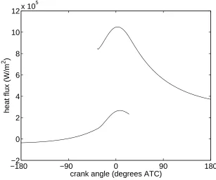
[1] conrms that the present implementation produces the expected results. Figure 11 indicates

theheatux withintheburned and unburned zonesforthefergusoncase. Toproducetheseheat

uxresults, an additionalfunction,calcq.m (AppendixJ) isusedto post-processthe results.

The indicated mean eective pressurefrom the current calculations is 0.95278MPa whereas F

er-guson[1 ]obtainsavalueof0.95102MPa{adierenceofaround0.2%. Errorsintheconservation

of mass(error1) andenergy (error2)are around0.04%forthecurrentcalculations.

7 Conclusions

A numberof Matlabfunctions andscript leshavebeenwrittento simulate thethermodynamics

of spark ignition internal combustion engines, based on the various FORTRAN codes described

[image:13.595.136.446.85.337.2]

(14)

−180

0

−90

0

90

180

500

1000

1500

2000

2500

3000

crank angle (degrees ATC)

temperature (K)

burned gas

unburned gas

Figure7: Temperature fromahrind.m(lines)and Ferguson [1 ](symbols).

−180

−90

0

90

180

−300

−150

0

150

300

450

600

crank angle (degrees ATC)

[image:14.595.138.445.110.353.2] [image:14.595.141.444.456.696.2]

(15)

−180

−90

0

90

180

−50

0

50

100

150

200

250

300

heat transfer (J)

Figure 9: Heat transferfrom ahrind.m(line) andFerguson[1 ] (symbols).

−180

−8

−90

0

90

180

−7

−6

−5

−4

−3

−2

−1

0

[image:15.595.138.446.107.352.2] [image:15.595.139.446.451.703.2]

(16)

−180

−2

−90

0

90

180

0

2

4

6

8

10

12

x 10

5

heat flux (W/m

2

)

Figure 11: Heatux resultsfromahrind.m.

The accuracy of thecurve coeÆcientsthat areused to describe thethermodynamicproperties of

the fuel, air, and combustion products has been established through internal consistency checks

and comparisons to well established properties at the reference conditions, T = 298:15K and

p = 101:325kPa. Based on these results, it is concluded that the fundamental thermodynamic

propertiesof thefuel,air,and combustion productspeciesareinagreement withpreviously

pub-lished resultsto withinthe scatterof those results{typicallylessthan 1%.

The accuracy of the Matlab equilibrium combustion products routine was established through

comparison with a comparable FORTRAN routine (Turns [7 ]) which has been revised over a

numberof years. Maximum dierences inmolar concentrations of less than 0.2%were typically

apparentovertherangeofconditionscalculatedbythetworoutines. Adiabaticametemperature

calculations also conrmed that dierences between the new Matlab routines and established

resultsaretypicallylessthanthe round-oerrors intheestablishedresults{ around0.05%.

ComparisonofanexampleenginecalculationusingthenewMatlabroutinesandtheoriginalresults

obtainedbyFerguson[1 ]demonstratesthatroutinesproduceaccurateresults. Theindicatedmean

eective pressurecalculatedbythetwo methodsdiersbyaround0.2%.

References

[1] C. R. Ferguson, Internal Combustion Engines, Applied Thermosciences, John Wiley and

Sons,New York,1986.

[2] S. Gordon and B. J. McBride, \Computer Program for Calculation of Complex Chemical

[image:16.595.138.445.84.340.2]

(17)

Chapman-[3] \JANAFThermochemicalTables", U.S NationalBureauof StandardsPublications

NSRDS-NBS37,June 1971.

[4] R. J. Kee, F. M. Rupley, and J. A. Miller, \The Chemkin Thermodynamic Data Base",

SandiaReportSAND87-8215B, March 1991.

[5] J.B. Heywood, Internal Combustion EngineFundamentals, McGraw-Hill,New York,1988.

[6] R.Stone, Introduction toInternal Combustion Engines, MacmillanPress,Basingstoke, third

edition,1999.

[7] S.R.Turns, An Introduction toCombustion, Concepts and Applications, McGraw-Hill,New

York, 1996.

[8] R.R.Raine, \ISIS_319UserManual,computermodellingofnitricoxideformationinaspark

ignitionengine", Report, Revision3,Oxford Engine Group,October2000.

[9] S. D. Hires, A. Ekchian, J. B. Heywood, R. J. Tabaczynski, and J. C. Wall, \Performance

andNOxEmissionsModelingofaJetIgnitionPre-ChamberStratiedChargeEngine", SAE

Transactions, vol. 85,Paper760161, 1976.

[10] C. Olikaraand G. L.Borman, \Calculating Properties of EquilibriumCombustion Products

withSome Applicationsto I.C.Engines", SAEPaper750468, 1975.

[11] G.Woschni, \A UniversallyApplicableEquation fortheInstantaneousHeatTransfer

(18)

A airdata.m

function A=airdata(scheme);

%

% A=airdata(scheme)

%

% Routine to specify the thermodynamic properties of air and

% combustion products.

% Data taken from:

% 1. Gordon, S., and McBride, B. J., 1971, "Computer Program for

% Calculation of Complex Chemical Equilibrium Composition, Rocket

% Performance, Incident and Reflected Shocks, and Chapman-Jouguet

% Detonations," NASA SP-273. As reported in Ferguson, C. R., 1986,

% "Internal Combustion Engines", Wiley.

% 2. Kee, R. J., et al., 1991, "The Chemkin Thermodynamic Data Base",

% Sandia Report, SAND87-8215B. As reported in

% Turns, S. R., 1996, "An Introduction to Combustion:

% Concepts and Applications", McGraw-Hill.

% ********************************************************************

% input:

% scheme switch:

% 'GMcB_low' - Gordon and McBride 300 < T < 1000 K

% 'GMcB_hi' - Gordon and McBride 1000 < T < 5000 K

% 'Chemkin_low' - Chemkin 300 < T < 1000 K

% 'Chemkin_hi' - Chemkin 1000 < T < 5000 K

% output:

% A - matrix of polynomial coefficients for cp/R, h/RT, and s/R

% of the form h/RT=a1+a2*T/2+a3*T^2/3+a4*T^3/4+a5*T^4/5*a6/T (for

% example) where T is expressed in K

% columns 1 to 7 are coefficients a1 to a7, and

% rows 1 to 10 are species CO2 H2O N2 O2 CO H2 H O OH and NO

% ********************************************************************

switch scheme

case 'GMcB_low'

A=[ 0.24007797E+01 0.87350957E-02 -0.66070878E-05 0.20021861E-08 ...

0.63274039E-15 -0.48377527E+05 0.96951457E+01

0.40701275E+01 -0.11084499E-02 0.41521180E-05 -0.29637404E-08 ...

0.80702103E-12 -0.30279722E+05 -0.32270046E+00

0.36748261E+01 -0.12081500E-02 0.23240102E-05 -0.63217559E-09 ...

-0.22577253E-12 -0.10611588E+04 0.23580424E+01

0.36255985E+01 -0.18782184E-02 0.70554544E-05 -0.67635137E-08 ...

0.21555993E-11 -0.10475226E+04 0.43052778E+01

0.37100928E+01 -0.16190964E-02 0.36923594E-05 -0.20319674E-08 ...

0.23953344E-12 -0.14356310E+05 0.29555350E+01

0.30574451E+01 0.26765200E-02 -0.58099162E-05 0.55210391E-08 ...

-0.18122739E-11 -0.98890474E+03 -0.22997056E+01

(19)

0.29464287E+01 -0.16381665E-02 0.24210316E-05 -0.16028432E-08 ...

0.38906964E-12 0.29147644E+05 0.29639949E+01

0.38375943E+01 -0.10778858E-02 0.96830378E-06 0.18713972E-09 ...

-0.22571094E-12 0.36412823E+04 0.49370009E+00

0.40459521E+01 -0.34181783E-02 0.79819190E-05 -0.61139316E-08 ...

0.15919076E-11 0.97453934E+04 0.29974988E+01];

case 'GMcB_hi'

A=[ 0.44608041E+01 0.30981719E-02 -0.12392571E-05 0.22741325E-09 ...

-0.15525954E-13 -0.48961442E+05 -0.98635982E+00

0.27167633E+01 0.29451374E-02 -0.80224374E-06 0.10226682E-09 ...

-0.48472145E-14 -0.29905826E+05 0.66305671E+01

0.28963194E+01 0.15154866E-02 -0.57235277E-06 0.99807393E-10 ...

-0.65223555E-14 -0.90586184E+03 0.61615148E+01

0.36219535E+01 0.73618264E-03 -0.19652228E-06 0.36201558E-10 ...

-0.28945627E-14 -0.12019825E+04 0.36150960E+01

0.29840696E+01 0.14891390E-02 -0.57899684E-06 0.10364577E-09 ...

-0.69353550E-14 -0.14245228E+05 0.63479156E+01

0.31001901E+01 0.51119464E-03 0.52644210E-07 -0.34909973E-10 ...

0.36945345E-14 -0.87738042E+03 -0.19629421E+01

0.25000000E+01 0.00000000E+00 0.00000000E+00 0.00000000E+00 ...

0.00000000E+00 0.25471627E+05 -0.46011763E+00

0.25420596E+01 -0.27550619E-04 -0.31028033E-08 0.45510674E-11 ...

-0.43680515E-15 0.29230803E+05 0.49203080E+01

0.29106427E+01 0.95931650E-03 -0.19441702E-06 0.13756646E-10 ...

0.14224542E-15 0.39353815E+04 0.54423445E+01

0.31890000E+01 0.13382281E-02 -0.52899318E-06 0.95919332E-10 ...

-0.64847932E-14 0.98283290E+04 0.67458126E+01];

case 'Chemkin_low'

A=[ 0.02275724E+02 0.09922072E-01 -0.10409113E-04 0.06866686E-07 ...

-0.02117280E-10 -0.04837314E+06 0.10188488E+02

0.03386842E+02 0.03474982E-01 -0.06354696E-04 0.06968581E-07 ...

-0.02506588E-10 -0.03020811E+06 0.02590232E+02

0.03298677E+02 0.14082404E-02 -0.03963222E-04 0.05641515E-07 ...

-0.02444854E-10 -0.10208999E+04 0.03950372E+02

0.03212936E+02 0.11274864E-02 -0.05756150E-05 0.13138773E-08 ...

-0.08768554E-11 -0.10052490E+04 0.06034737E+02

0.03262451E+02 0.15119409E-02 -0.03881755E-04 0.05581944E-07 ...

-0.02474951E-10 -0.14310539E+05 0.04848897E+02

0.03298124E+02 0.08249441E-02 -0.08143015E-05 -0.09475434E-09 ...

0.04134872E-11 -0.10125209E+04 -0.03294094E+02

0.02500000E+02 0.00000000E+00 0.00000000E+00 0.00000000E+00 ...

0.00000000E+00 0.02547162E+06 -0.04601176E+01

0.02946428E+02 -0.16381665E-02 0.02421031E-04 -0.16028431E-08 ...

0.03890696E-11 0.02914764E+06 0.02963995E+02

0.03637266E+02 0.01850910E-02 -0.16761646E-05 0.02387202E-07 ...

-0.08431442E-11 0.03606781E+05 0.13588605E+01

0.03376541E+02 0.12530634E-02 -0.03302750E-04 0.05217810E-07 ...

-0.02446262E-10 0.09817961E+05 0.05829590E+02];

(20)

-0.16690333E-13 -0.04896696E+06 -0.09553959E+01

0.02672145E+02 0.03056293E-01 -0.08730260E-05 0.12009964E-09 ...

-0.06391618E-13 -0.02989921E+06 0.06862817E+02

0.02926640E+02 0.14879768E-02 -0.05684760E-05 0.10097038E-09 ...

-0.06753351E-13 -0.09227977E+04 0.05980528E+02

0.03697578E+02 0.06135197E-02 -0.12588420E-06 0.01775281E-09 ...

-0.11364354E-14 -0.12339301E+04 0.03189165E+02

0.03025078E+02 0.14426885E-02 -0.05630827E-05 0.10185813E-09 ...

-0.06910951E-13 -0.14268350E+05 0.06108217E+02

0.02991423E+02 0.07000644E-02 -0.05633828E-06 -0.09231578E-10 ...

0.15827519E-14 -0.08350340E+04 -0.13551101E+01

0.02500000E+02 0.00000000E+00 0.00000000E+00 0.00000000E+00 ...

0.00000000E+00 0.02547162E+06 -0.04601176E+01

0.02542059E+02 -0.02755061E-03 -0.03102803E-07 0.04551067E-10 ...

-0.04368051E-14 0.02923080E+06 0.04920308E+02

0.02882730E+02 0.10139743E-02 -0.02276877E-05 0.02174683E-09 ...

-0.05126305E-14 0.03886888E+05 0.05595712E+02

0.03245435E+02 0.12691383E-02 -0.05015890E-05 0.09169283E-09 ...

-0.06275419E-13 0.09800840E+05 0.06417293E+02];

end

B fueldata.m

function [alpha,beta,gamma,delta,Afuel]=fueldata(fuel);

%

% [alpha,beta,gamma,delta,Afuel]=fueldata(fuel)

%

% Routine to specify the thermodynamic properties of a fuel.

% Data taken from:

% 1. Ferguson, C.R., 1986, "Internal Combustion Engines", Wiley;

% 2. Heywood, J.B., 1988, "Internal Combustion Engine Fundamentals",

% McGraw-Hill; and

% 3. Raine, R. R., 2000, "ISIS_319 User Manual", Oxford Engine Group.

% ********************************************************************

% input:

% fuel switch

% from Ferguson: 'gasoline', 'diesel', 'methane', 'methanol',

% 'nitromethane', 'benzene';

% from Heywood: 'methane_h', 'propane', 'hexane', 'isooctane_h',

% 'methanol_h', 'ethanol', 'gasoline_h1', gasoline_h2', 'diesel_h';

% from Raine: 'toluene', 'isooctane'.

% output:

% alpha, beta, gamma, delta - number of C, H, 0, and N atoms

% Afuel - vector of polynomial coefficients for cp/R, h/RT, and s/R

% of the form h/RT=a1+a2*T/2+a3*T^2/3+a4*T^3/4-a5/T^2+a6/T (for

(21)

% Set values for conversion of Heywood data to nondimensional format

% with T expressed in K

SVal=4.184e3/8.31434;

SVec=SVal*[1e-3 1e-6 1e-9 1e-12 1e3 1 1];

switch fuel

case 'gasoline' % Ferguson

alpha=7; beta=17; gamma=0; delta=0;

Afuel=[4.0652 6.0977E-02 -1.8801E-05 0 0 -3.5880E+04 15.45];

case 'diesel' % Ferguson

alpha=14.4; beta=24.9; gamma=0; delta=0;

Afuel=[7.9710 1.1954E-01 -3.6858E-05 0 0 -1.9385E+04 -1.7879];

case 'methane' % Ferguson

Afuel=[1.971324 7.871586E-03 -1.048592E-06 0 0 -9.930422E+03 8.873728];

case 'methanol' % Ferguson

Afuel=[1.779819 1.262503E-02 -3.624890E-06 0 0 -2.525420E+04 1.50884E+01];

case 'nitromethane' % Ferguson

Afuel=[1.412633 2.087101E-02 -8.142134E-06 0 0 -1.026351E+04 1.917126E+01];

case 'benzene' % Ferguson

Afuel=[-2.545087 4.79554E-02 -2.030765E-05 0 0 8.782234E+03 3.348825E+01];

case 'toluene' % Raine

Afuel=[-2.09053 5.654331e-2 -2.350992e-5 0 0 4331.441411 34.55418257];

case 'isooctane' % Raine

Afuel=[6.678E-1 8.398E-2 -3.334E-5 0 0 -3.058E+4 2.351E+1];

case 'methane_h' % Heywood

Afuel=[-0.29149 26.327 -10.610 1.5656 0.16573 -18.331 19.9887/SVal].*SVec;

case 'propane' % Heywood

Afuel=[-1.4867 74.339 -39.065 8.0543 0.01219 -27.313 26.4796/SVal].*SVec;

case 'hexane' % Heywood

Afuel=[-20.777 210.48 -164.125 52.832 0.56635 -39.836 79.5542/SVal].*SVec;

case 'isooctane_h' % Heywood

Afuel=[-0.55313 181.62 -97.787 20.402 -0.03095 -60.751 27.2162/SVal].*SVec;

case 'methanol_h' % Heywood

Afuel=[-2.7059 44.168 -27.501 7.2193 0.20299 -48.288 31.1406/SVal].*SVec;

case 'ethanol' % Heywood

Afuel=[6.990 39.741 -11.926 0 0 -60.214 8.01623/SVal].*SVec;

(22)

Afuel=[-24.078 256.63 -201.68 64.750 0.5808 -27.562 NaN].*SVec;

case 'gasoline_h2' % Heywood

Afuel=[-22.501 227.99 -177.26 56.048 0.4845 -17.578 NaN].*SVec;

case 'diesel_h' % Heywood

Afuel=[-9.1063 246.97 -143.74 32.329 0.0518 -50.128 NaN].*SVec;

end

C farg.m

function [h,u,v,s,Y,cp,dlvlT,dlvlp]=farg(p,T,phi,f,fueltype,airscheme);

%

% [h,u,v,s,Y,cp,dlvlT,dlvlp]=farg(p,T,phi,f,fueltype,airscheme)

%

% Routine to determine the state of mixtures of fuel, air

% and residual combustion products at low temperatures.

% Method closely follows that of:

% 1. Ferguson, C.R., 1986, "Internal Combustion Engines", Wiley, p108;

% who uses the results of:

% 2. Hires, S.D., Ekchian, A., Heywood, J.B., Tabaczynski, R.J., and

% Wall, J.C., 1976, "Performance and NOx Emissions Modeling of a Jet

% Ignition Pre-Chamber Stratified Charge Engine", SAE Trans., Vol 85,

% Paper 760161.

% ********************************************************************

% input:

% p,T,phi - pressure (Pa), temperature (K), and equivalence ratio

% f - residual mass fraction; set f=0 if no combustion products

% are present and f=1 if only combustion products are present

% fueltype - 'gasoline', 'diesel', etc - see fueldata.m for full list

% airscheme - 'GMcB' (Gordon and McBride) or 'Chemkin'

% output:

% h - enthalpy (J/kg), u - internal energy (J/kg),

% v - specific volume (m^3/kg), s - entropy (J/kgK),

% Y - mole fractions of 6 species: CO2, H2O, N2, O2, CO, and H2,

% cp - specific heat (J/kgK),

% dlvlT - partial derivative of log(v) wrt log(T)

% dlvlp - partial derivative of log(v) wrt log(p)

% ********************************************************************

[alpha,beta,gamma,delta,Afuel]=fueldata(fueltype);

switch airscheme

case 'GMcB'

A=airdata('GMcB_low');

case 'Chemkin'

(23)

Ru=8314.34; % J/kmolK

table=[-1 1 0 0 1 -1]';

M=[44.01 18.02 28.008 32.000 28.01 2.018]'; % kg/kmol

MinMol=1e-25;

dlvlT=1; dlvlp=-1;

eps=0.210/(alpha+0.25*beta-0.5*gamma);

if phi <= 1.0 % stoichiometric or lean

nu=[alpha*phi*eps beta*phi*eps/2 0.79+delta*phi*eps/2 ...

0.21*(1-phi) 0 0]';

dcdT=0;

else % rich

z=1000/T;

K=exp(2.743+z*(-1.761+z*(-1.611+z*0.2803)));

dKdT=-K*(-1.761+z*(-3.222+z*0.8409))/1000;

a=1-K;

b=0.42-phi*eps*(2*alpha-gamma)+K*(0.42*(phi-1)+alpha*phi*eps);

c=-0.42*alpha*phi*eps*(phi-1)*K;

nu5=(-b+sqrt(b^2-4*a*c))/2/a;

dcdT=dKdT*(nu5^2-nu5*(0.42*(phi-1)+alpha*phi*eps)+ ...

0.42*alpha*phi*eps*(phi-1))/(2*nu5*a+b);

nu=[alpha*phi*eps-nu5 0.42-phi*eps*(2*alpha-gamma)+nu5 ...

0.79+delta*phi*eps/2 0 nu5 0.42*(phi-1)-nu5]';

end

% mole fractions and molecular weight of residual

tmoles=sum(nu);

Y=nu/tmoles;

Mres=sum(Y.*M);

% mole fractions and molecular weight of fuel-air

fuel=eps*phi/(1+eps*phi);

o2=0.21/(1+eps*phi);

n2=0.79/(1+eps*phi);

Mfa=fuel*(12.01*alpha+1.008*beta+16*gamma+14.01*delta)+ ...

32*o2+28.02*n2;

% mole fractions of fuel-air-residual gas

Yres=f/(f+Mres/Mfa*(1-f));

Y=Y*Yres;

Yfuel=fuel*(1-Yres);

Y(3)=Y(3)+n2*(1-Yres);

Y(4)=Y(4)+o2*(1-Yres);

% component properties

Tcp0=[1 T T^2 T^3 T^4]';

(24)

cp0=A(1:6,1:5)*Tcp0;

h0=A(1:6,1:6)*Th0;

s0=A(1:6,[1:5 7])*Ts0;

Mfuel=12.01*alpha+1.008*beta+16.000*gamma+14.01*delta;

a0=Afuel(1); b0=Afuel(2); c0=Afuel(3); d0=Afuel(6); e0=Afuel(7);

cpfuel=Afuel(1:5)*[1 T T^2 T^3 1/T^2]';

hfuel=Afuel(1:6)*[1 T/2 T^2/3 T^3/4 -1/T^2 1/T]';

s0fuel=Afuel([1:5 7])*[log(T) T T^2/2 T^3/3 -1/T^2/2 1]';

% set min value of composition so log calculations work

if Yfuel<MinMol

Yfuel=MinMol;

end

i=find(Y<MinMol);

Y(i)=ones(length(i),1)*MinMol;

% properties of mixture

h=hfuel*Yfuel+sum(h0.*Y);

s=(s0fuel-log(Yfuel))*Yfuel+sum((s0-log(Y)).*Y);

cp=cpfuel*Yfuel+sum(cp0.*Y)+sum(h0.*table*T*dcdT*Yres/tmoles);

MW=Mfuel*Yfuel+sum(Y.*M);

R=Ru/MW;

h=R*T*h;

u=h-R*T;

v=R*T/p;

s=R*(-log(p/101.325e3)+s);

cp=R*cp;

D ecp.m

function [h,u,v,s,Y,cp,dlvlT,dlvlp]=ecp(p,T,phi,fueltype,airscheme,Yguess);

%

% [h,u,v,s,Y,cp,dlvlT,dlvlp]=ecp(p,T,phi,fueltype,airscheme,Yguess)

%

% Routine to determine the equilibrium state of combustion products.

% Method closely follows that of:

% 1. Ferguson, C.R., 1986, "Internal Combustion Engines", Wiley, p122;

% which uses the method described by:

% 2. Olikara, C., and Borman, G.L., 1975, "A Computer Program for

% Calculating Properties of Equilibrium Combustion Products with

% Some Applications to I.C. Engines", SAE Paper 750468.

% ********************************************************************

% input:

% p,T,phi - pressure (Pa), temperature (K), and equivalence ratio

(25)

% species CO2 H2O N2 O2 CO H2 H O OH and NO

% output:

% h - enthalpy (J/kg), u - internal energy (J/kg),

% v - specific volume (m^3/kg), s - entropy (J/kgK),

% Y - mole fractions of 10 species, cp - specific heat (J/kgK),

% dlvlT - partial derivative of log(v) wrt log(T)

% dlvlp - partial derivative of log(v) wrt log(p)

% ********************************************************************

[alpha,beta,gamma,delta,Afuel]=fueldata(fueltype);

switch airscheme

case 'GMcB'

A0=airdata('GMcB_hi');

case 'Chemkin'

A0=airdata('Chemkin_hi');

end

% Equilibrium constant data from Olikara and Borman via Ferguson

Kp=[ 0.432168E+00 -0.112464E+05 0.267269E+01 -0.745744E-04 0.242484E-08

0.310805E+00 -0.129540E+05 0.321779E+01 -0.738336E-04 0.344645E-08

-0.141784E+00 -0.213308E+04 0.853461E+00 0.355015E-04 -0.310227E-08

0.150879E-01 -0.470959E+04 0.646096E+00 0.272805E-05 -0.154444E-08

-0.752364E+00 0.124210E+05 -0.260286E+01 0.259556E-03 -0.162687E-07

-0.415302E-02 0.148627E+05 -0.475746E+01 0.124699E-03 -0.900227E-08];

MinMol=1e-25;

tol=3e-12;

Ru=8314.34; % J/kmol.K

M=[44.01 18.02 28.008 32.000 28.01 2.018 1.009 16 17.009 30.004]'; % kg/kmol

dcdT=zeros(4,1);

dcdp=zeros(4,1);

dfdT=zeros(4,1);

dfdp=zeros(4,1);

dYdT=zeros(10,1);

dYdp=zeros(10,1);

B=zeros(4,1);

% check if solid carbon will form

eps=0.210/(alpha+0.25*beta-0.5*gamma);

if phi>(0.210/eps/(0.5*alpha-0.5*gamma))

error('phi too high - c(s) and other species will form');

end

if nargin==5 % no Yguess so estimate the composition using farg

[h,u,v,s,Y,cp,dlvlT,dlvlp]=farg(p,T,phi,1,fueltype,airscheme);

Y(7:10)=ones(4,1)*MinMol; % since farg only returns first 6 species

(26)

end

% evaluate constants

patm=p/101.325e3; % convert Pa to atmospheres

TKp=[log(T/1000) 1/T 1 T T^2]';

K=10.^(Kp*TKp);

c=K.*[1/sqrt(patm) 1/sqrt(patm) 1 1 sqrt(patm) sqrt(patm)]';

d=[beta/alpha (gamma+0.42/eps/phi)/alpha (delta+1.58/eps/phi)/alpha]';

if abs(phi-1)<tol

phi=phi*(1+tol*sign(phi-1));

end

i=find(Y<MinMol);

DY3to6=2*tol*ones(4,1);

MaxIter=500;

MaxVal=max(abs(DY3to6));

Iter=0;

DoneSome=0;

while (Iter<MaxIter)&((MaxVal>tol)|(DoneSome<1))

Iter=Iter+1;

if Iter>2,

DoneSome=1;

end

D76=0.5*c(1)/sqrt(Y(6));

D84=0.5*c(2)/sqrt(Y(4));

D94=0.5*c(3)*sqrt(Y(6)/Y(4));

D96=0.5*c(3)*sqrt(Y(4)/Y(6));

D103=0.5*c(4)*sqrt(Y(4)/Y(3));

D104=0.5*c(4)*sqrt(Y(3)/Y(4));

D24=0.5*c(5)*Y(6)/sqrt(Y(4));

D26=c(5)*sqrt(Y(4));

D14=0.5*c(6)*Y(5)/sqrt(Y(4));

D15=c(6)*sqrt(Y(4));

A(1,1)=1+D103;

A(1,2)=D14+D24+1+D84+D104+D94;

A(1,3)=D15+1;

A(1,4)=D26+1+D76+D96;

A(2,1)=0;

A(2,2)=2*D24+D94-d(1)*D14;

A(2,3)=-d(1)*D15-d(1);

A(2,4)=2*D26+2+D76+D96;

A(3,1)=D103;

A(3,2)=2*D14+D24+2+D84+D94+D104-d(2)*D14;

(27)

A(4,1)=2+D103;

A(4,2)=D104-d(3)*D14;

A(4,3)=-d(3)*D15-d(3);

A(4,4)=0;

B(1)=-(sum(Y)-1);

B(2)=-(2*Y(2)+2*Y(6)+Y(7)+Y(9)-d(1)*Y(1)-d(1)*Y(5));

B(3)=-(2*Y(1)+Y(2)+2*Y(4)+Y(5)+Y(8)+Y(9)+Y(10)-d(2)*Y(1)-d(2)*Y(5));

B(4)=-(2*Y(3)+Y(10)-d(3)*Y(1)-d(3)*Y(5));

invA=inv(A);

DY3to6=invA*B;

MaxVal=max(abs(DY3to6));

Y(3:6)=Y(3:6)+DY3to6/10;

i=find(Y<MinMol);

Y(7)=c(1)*sqrt(Y(6));

Y(8)=c(2)*sqrt(Y(4));

Y(9)=c(3)*sqrt(Y(4)*Y(6));

Y(10)=c(4)*sqrt(Y(4)*Y(3));

Y(2)=c(5)*sqrt(Y(4))*Y(6);

Y(1)=c(6)*sqrt(Y(4))*Y(5);

end

if Iter>=MaxIter

warning('convergence failure in composition loop');

end

TdKdT=[1/T -1/T^2 1 2*T]';

dKdT=2.302585*K.*(Kp(:,[1 2 4 5])*TdKdT);

dcdT(1)=dKdT(1)/sqrt(patm);

dcdT(2)=dKdT(2)/sqrt(patm);

dcdT(3)=dKdT(3);

dcdT(4)=dKdT(4);

dcdT(5)=dKdT(5)*sqrt(patm);

dcdT(6)=dKdT(6)*sqrt(patm);

dcdp(1)=-0.5*c(1)/p;

dcdp(2)=-0.5*c(2)/p;

dcdp(5)=0.5*c(5)/p;

dcdp(6)=0.5*c(6)/p;

x1=Y(1)/c(6);

x2=Y(2)/c(5);

x7=Y(7)/c(1);

x8=Y(8)/c(2);

x9=Y(9)/c(3);

x10=Y(10)/c(4);

dfdT(1)=dcdT(6)*x1+dcdT(5)*x2+dcdT(1)*x7+dcdT(2)*x8+ ...

dcdT(3)*x9+dcdT(4)*x10;

(28)

dcdT(4)*x10-d(2)*dcdT(6)*x1;

dfdT(4)=dcdT(4)*x10-d(3)*dcdT(6)*x1;

dfdp(1)=dcdp(6)*x1+dcdp(5)*x2+dcdp(1)*x7+dcdp(2)*x8;

dfdp(2)=2*dcdp(5)*x2+dcdp(1)*x7-d(1)*dcdp(6)*x1;

dfdp(3)=2*dcdp(6)*x1+dcdp(5)*x2+dcdp(2)*x8-d(2)*dcdp(6)*x1;

dfdp(4)=-d(3)*dcdp(6)*x1;

B=-dfdT;

dYdT(3:6)=invA*B;

dYdT(1)=sqrt(Y(4))*Y(5)*dcdT(6)+D14*dYdT(4)+D15*dYdT(5);

dYdT(2)=sqrt(Y(4))*Y(6)*dcdT(5)+D24*dYdT(4)+D26*dYdT(6);

dYdT(7)=sqrt(Y(6))*dcdT(1)+D76*dYdT(6);

dYdT(8)=sqrt(Y(4))*dcdT(2)+D84*dYdT(4);

dYdT(9)=sqrt(Y(4)*Y(6))*dcdT(3)+D94*dYdT(4)+D96*dYdT(6);

dYdT(10)=sqrt(Y(4)*Y(3))*dcdT(4)+D104*dYdT(4)+D103*dYdT(3);

B=-dfdp;

dYdp(3:6)=invA*B;

dYdp(1)=sqrt(Y(4))*Y(5)*dcdp(6)+D14*dYdp(4)+D15*dYdp(5);

dYdp(2)=sqrt(Y(4))*Y(6)*dcdp(5)+D24*dYdp(4)+D26*dYdp(6);

dYdp(7)=sqrt(Y(6))*dcdp(1)+D76*dYdp(6);

dYdp(8)=sqrt(Y(4))*dcdp(2)+D84*dYdp(4);

dYdp(9)=D94*dYdp(4)+D96*dYdp(6);

dYdp(10)=D104*dYdp(4)+D103*dYdp(3);

% calculate thermodynamic properties

Tcp0=[1 T T^2 T^3 T^4]';

Th0=[1 T/2 T^2/3 T^3/4 T^4/5 1/T]';

Ts0=[log(T) T T^2/2 T^3/3 T^4/4 1]';

cp0=A0(:,1:5)*Tcp0;

h0=A0(:,1:6)*Th0;

s0=A0(:,[1:5 7])*Ts0;

% Y(1) and Y(2) reevaluated

Y(1)=(2*Y(3)+Y(10))/d(3)-Y(5);

Y(2)=(d(1)/d(3)*(2*Y(3)+Y(10))-2*Y(6)-Y(7)-Y(9))/2;

i=find(Y<MinMol);

% properties of mixture

h=sum(h0.*Y);

s=sum((s0-log(Y)).*Y);

cp=sum(Y.*cp0+h0.*dYdT*T);

MW=sum(Y.*M);

MT=sum(dYdT.*M);

Mp=sum(dYdp.*M);

R=Ru/MW;

(29)

dlvlT=1+max(-T*MT/MW,0);

dlvlp=-1-max(p*Mp/MW,0);

h=R*T*h;

s=R*(-log(patm)+s);

u=h-R*T;

E Tadiabatic.m

function Tb=Tadiabatic(p,Tu,phi,f,fueltype,airscheme);

%

% Tb=Tadiabatic(p,Tu,phi,f,fueltype,airscheme)

%

% Routine for calculating the adiabatic flame temperature.

% Method involves iteratively selecting flame temperatures until

% the enthalpy of the combustion products (in equilibrium) matches

% the enthalpy of the initial gas mixture.

% farg.m is used to determine the enthalpy of the unburned mixture,

% and ecp.m is used to determine the enthalpy of the burned gas.

% ********************************************************************

% input:

% p - pressure (Pa)

% Tu - temperature of the unburned mixture (K)

% phi - equivalence ratio

% f - residual mass fraction; set f=0 if no combustion products

% are present and f=1 if only combustion products are present

% airscheme - 'GMcB' (Gordon and McBride) or 'Chemkin'

% output:

% Tb - temperature of the burned gas (K) - adiabatic flame temperature

% ********************************************************************

MaxIter=50;

Tol=0.00001; % 0.001% allowable error in temperature calculation

Tb=2000; % initial estimate

DeltaT=2*Tol*Tb; % something big

Iter=0;

[hu,u,v,s,Y,cp,dlvlT,dlvlp]=farg(p,Tu,phi,f,fueltype,airscheme);

while (Iter<MaxIter)&(abs(DeltaT/Tb)>Tol)

Iter=Iter+1;

[hb,u,v,s,Y,cp,dlvlT,dlvlp]=ecp(p,Tb,phi,fueltype,airscheme);

DeltaT=(hu-hb)/cp;

Tb=Tb+DeltaT;

end

if Iter>=MaxIter

(30)

F enginedata.m

% enginedata.m

%

% Script file used by the function ahrind.m to

% define the engine properties and initial conditions

% ***** engine geometry **********************************************

b=0.1; % engine bore (m)

stroke=0.08; % engine stroke (m)

eps=0.25; % half stroke to rod ratio, s/2l

r=10; % compression ratio

Vtdc=pi/4*b^2*stroke/(r-1); % volume at TDC

Vbdc=pi/4*b^2*stroke+Vtdc; % volume at BDC

% ***** engine thermofluids parameters *******************************

Cblowby=0.8; % piston blowby constant (s^-1)

f=0.1; % residual fraction

fueltype='gasoline';

airscheme='GMcB';

phi=0.8; % equivalence ratio

thetas=-35*pi/180; % start of burning

thetab=60*pi/180; % burn duration angle

RPM=2000;

omega=RPM*pi/30; % engine speed in rad/s

heattransferlaw='constant'; % 'constant', or 'Woschni'

hcu=500; % unburned zone heat transfer coefficient/weighting

hcb=500; % burned zone heat transfer coefficient/weighting

Tw=420; % engine surface temperature

% ***** initial conditions *******************************************

p1=100e3;

T1=350;

theta1=-pi;

V1=Vbdc;

[h1,u1,v1,s1,Y1,cp1,dlvlT1,dlvlp1]=farg(p1,T1,phi,f,fueltype,airscheme);

mass1=Vbdc/v1;

U1=u1*mass1;

G RatesComp.m & RatesComb.m & RatesExp.m

function yprime=RatesComp(theta,y,flag);

%

% yprime=RatesComp(theta,y,flag)

%

(31)

% 1) pressure; 2) unburned temperature;

% 3) work; 4) heat transfer; and 5) heat leakage.

% See Ferguson, C.R., 1986, "Internal Combustion Engines", Wiley,

% p174.

global b stroke eps r Cblowby f fueltype airscheme phi ...

thetas thetab omega ...

heattransferlaw hcu ...

Tw theta1 Vtdc mass1 ...

p=y(1);

Tu=y(2);

yprime=zeros(5,1);

% mass in cylinder accounting for blowby:

mass=mass1*exp(-Cblowby*(theta-theta1)/omega);

% volume of cylinder:

V=Vtdc*(1+(r-1)/2*(1-cos(theta)+ ...

1/eps*(1-(1-eps^2*sin(theta).^2).^0.5)));

% derivate of volume:

dVdtheta=Vtdc*(r-1)/2*(sin(theta)+ ...

eps/2*sin(2*theta)./sqrt(1-eps^2*sin(theta).^2));

switch heattransferlaw

case 'constant'

hcoeff=hcu;

case 'Woschni'

upmean=omega*stroke/pi; % mean piston velocity

C1=2.28;

hcoeff=hcu*130*b^(-0.2)*Tu^(-0.53)*(p/100e3)^(0.8)*C1*upmean;

end

A=1/mass*(dVdtheta+V*Cblowby/omega);

Qconv=hcoeff*(pi*b^2/2+4*V/b)*(Tu-Tw);

Const1=1/omega/mass;

[h,u,v,s,Y,cp,dlvlT,dlvlp]=farg(p,Tu,phi,f,fueltype,airscheme);

B=Const1*v/cp*dlvlT*Qconv/Tu; % note typo on p174, eq. 4.76

C=0;

D=0;

E=v^2/cp/Tu*dlvlT^2+v/p*dlvlp;

yprime(1)=(A+B+C)/(D+E);

yprime(2)=-Const1/cp*Qconv+v/cp*dlvlT*yprime(1);

yprime(3)=p*dVdtheta;

yprime(4)=Qconv/omega;

(32)

%

% yprime=RatesComb(theta,y,flag)

%

% Function that returns the drivatives of the following 6 variables

% w.r.t. crank angle (theta) for the combustion phase:

% 1) pressure; 2) unburned temperature; 3) burned temperature;

% p174.

thetas thetab RPM omega ...

heattransferlaw hcu hcb ...

p1 T1 V1 Tw theta1 Vtdc Vbdc mass1

p=y(1);

Tb=y(2);

Tu=y(3);

yprime=zeros(6,1);

% volume of cylinder:

V=Vtdc*(1+(r-1)/2*(1-cos(theta)+ ...

1/eps*(1-(1-eps^2*sin(theta).^2).^0.5)));

% mass fraction burned and derivative:

x=0.5*(1-cos(pi*(theta-thetas)/thetab));

dxdtheta=pi/2/thetab*sin(pi*(theta-thetas)/thetab);

if x<0.0001, x=0.0001; end;

if x>0.9999, x=0.9999; end;

case 'constant'

hcoeffu=hcu;

hcoeffb=hcb;

case 'Woschni'

C1=2.28;

C2=3.24e-3;

Vs=Vbdc-Vtdc;

k=1.3;

pm=p1*(V1/V)^k; % motoring pressure

hcoeffu=hcu*130*b^(-0.2)*Tu^(-0.53)*(p/100e3)^(0.8)* ...

(C1*upmean+C2*Vs*T1/p1/V1*(p-pm))^(0.8);

hcoeffb=hcb*130*b^(-0.2)*Tb^(-0.53)*(p/100e3)^(0.8)* ...

(33)

Qconvu=hcoeffu*(pi*b^2/2+4*V/b)*(1-sqrt(x))*(Tu-Tw);

Qconvb=hcoeffb*(pi*b^2/2+4*V/b)*sqrt(x)*(Tb-Tw);

[hu,uu,vu,s,Y,cpu,dlvlTu,dlvlpu]= ...

farg(p,Tu,phi,f,fueltype,airscheme);

[hb,ub,vb,s,Y,cpb,dlvlTb,dlvlpb]= ...

ecp(p,Tb,phi,fueltype,airscheme);

B=Const1*(vb/cpb*dlvlTb*Qconvb/Tb+ ...

vu/cpu*dlvlTu*Qconvu/Tu);

C=-(vb-vu)*dxdtheta-vb*dlvlTb*(hu-hb)/cpb/Tb*(dxdtheta- ...

(x-x^2)*Cblowby/omega);

D=x*(vb^2/cpb/Tb*dlvlTb^2+vb/p*dlvlpb);

E=(1-x)*(vu^2/cpu/Tu*dlvlTu^2+vu/p*dlvlpu);

yprime(2)=-Const1/cpb/x*Qconvb+vb/cpb*dlvlTb*yprime(1)+ ...

(hu-hb)/cpb*(dxdtheta/x-(1-x)*Cblowby/omega);

yprime(3)=-Const1/cpu/(1-x)*Qconvu+vu/cpu*dlvlTu*yprime(1);

yprime(5)=Const1*mass*(Qconvb+Qconvu);

yprime(6)=Cblowby*mass/omega*((1-x^2)*hu+x^2*hb);

function yprime=RatesExp(theta,y,flag);

%

% yprime=RatesExp(theta,y,flag)

%

% Function that returns the drivatives of the following 5 variables

% w.r.t. crank angle (theta) for the expansion phase:

% 1) pressure; 2) unburned temperature;

% p174.

thetas thetab RPM omega ...

heattransferlaw hcb ...

p1 T1 V1 Tw theta1 Vtdc Vbdc mass1

p=y(1);

Tb=y(2);

yprime=zeros(5,1);

(34)

1/eps*(1-(1-eps^2*sin(theta).^2).^0.5)));

case 'constant'

hcoeff=hcb;

case 'Woschni'

C1=2.28;

C2=3.24e-3;

Vs=Vbdc-Vtdc;

k=1.3;

pm=p1*(V1/V)^k; % motoring pressure

hcoeff=hcb*130*b^(-0.2)*Tb^(-0.53)*(p/100e3)^(0.8)* ...

(C1*upmean+C2*Vs*T1/p1/V1*(p-pm))^(0.8);

end

Qconv=hcoeff*(pi*b^2/2+4*V/b)*(Tb-Tw);

if Tb<1000

[h,u,v,s,Y,cp,dlvlT,dlvlp]=farg(p,Tb,phi,1,fueltype,airscheme);

else

[h,u,v,s,Y,cp,dlvlT,dlvlp]=ecp(p,Tb,phi,fueltype,airscheme);

end

B=Const1*v/cp*dlvlT*Qconv/Tb;

C=0;

D=v^2/cp/Tb*dlvlT^2+v/p*dlvlp;

E=0;

yprime(2)=-Const1/cp*Qconv+v/cp*dlvlT*yprime(1);

yprime(4)=Qconv/omega;

yprime(5)=Cblowby*mass/omega*h;

H ahrind.m

% ahrind.m

%

% Script file to determine the performance of a fuel inducted engine

% based on a (user-specified) arbitrary heat release profile as a

% function of crank angle.

(35)

% ********************************************************************

% input:

% enginedata.m - this is another script file that defines all of the

% relevant engine parameters and operating conditions.

% output:

% ahrind.mat - this file contains all of the variables. For plotting

% the results, see the example script file plotresults.m

% ********************************************************************

timestart=cputime;

thetas thetab omega ...

Tw theta1 Vtdc Vbdc mass1 ...

p1 T1 V1

% load the engine parameters and initial conditions

enginedata

case 'Woschni'

if (abs(hcu) > 10)|(abs(hcb) > 10),

warning('Woschni model with weighting factor > 10')

end

% integration parameters

dtheta=1*pi/180;

options=odeset('RelTol',1e-3);

% integration during compression phase

disp(['integrating over the compression phase']);

[thetacomp,pTuWQlHl]=ode45('RatesComp', ...

[-pi:dtheta:thetas],[p1 T1 0 0 0],options);

% specification of initial conditions at start of combustion phase

% b - beginning of combustion

pb=interp1(thetacomp,pTuWQlHl(:,1),thetas);

Tub=interp1(thetacomp,pTuWQlHl(:,2),thetas);

Tbb=Tadiabatic(pb,Tub,phi,f,fueltype,airscheme);

Wb=interp1(thetacomp,pTuWQlHl(:,3),thetas);

Qlb=interp1(thetacomp,pTuWQlHl(:,4),thetas);

Hlb=interp1(thetacomp,pTuWQlHl(:,5),thetas);

% integration during combustion phase

disp(['integrating over the combustion phase']);

(36)

% specification of initial conditions at start of expansion phase

% e - end of combustion / start of expansion

pe=interp1(thetacomb,pTbTuWQlHl(:,1),thetas+thetab);

Tbe=interp1(thetacomb,pTbTuWQlHl(:,2),thetas+thetab);

We=interp1(thetacomb,pTbTuWQlHl(:,4),thetas+thetab);

Qle=interp1(thetacomb,pTbTuWQlHl(:,5),thetas+thetab);

Hle=interp1(thetacomb,pTbTuWQlHl(:,6),thetas+thetab);

% integration during expansion phase

disp(['integrating over the expansion phase']);

[thetaexp,pTbWQlHl]=ode45('RatesExp', ...

[thetas+thetab:dtheta:pi],[pe Tbe We Qle Hle],options);

% error checks

mass4=mass1*exp(-Cblowby*2*pi/omega);

p4=interp1(thetaexp,pTbWQlHl(:,1),pi);

T4=interp1(thetaexp,pTbWQlHl(:,2),pi);

W4=interp1(thetaexp,pTbWQlHl(:,3),pi);

Ql4=interp1(thetaexp,pTbWQlHl(:,4),pi);

Hl4=interp1(thetaexp,pTbWQlHl(:,5),pi);

[h4,u4,v4,s4,Y4,cp4,dlvlT4,dlvlp4]= ...

farg(p4,T4,phi,1,fueltype,airscheme);

U4=u4*mass4;

error1=1-v4*mass4/Vbdc;

error2=1+W4/(U4-U1+Ql4+Hl4);

% indicated mean effective pressure and thermal efficiency

imep=W4/(pi*b^2/4*stroke);

eta=W4/mass1*(1+phi*0.06548*(1-f))/phi/0.06548/(1-f)/47870/1e3;

% calcuate the heat flux in W/m^2

qcomp=calcq(thetacomp,pTuWQlHl,'comp'); % compression

qcombu=calcq(thetacomb,pTbTuWQlHl,'combu'); % combustion-unburned zone

qcombb=calcq(thetacomb,pTbTuWQlHl,'combb'); % combustion-burned zone

qexp=calcq(thetaexp,pTbWQlHl,'exp'); % expansion

timefinish=cputime;

timetaken=timefinish-timestart;

% save all data

save ahrind.mat

clear

I plotresults.m

(37)

% Script file to plot output from ahrind.m and compare results

% with output listed in:

% Ferguson, C.R., 1986, "Internal Combustion Engines", Wiley, p178;

load ahrind.mat; % results from ahrind.mat

load ferguson.txt; % tabulated output from ferguson p178-179

% Set some parameters to make figures look attractive

NLW=1; % normal line width

NFS=18; % normal font size

NMS=1; % normal marker size

close all;

figure(1);

plot(thetacomp*180/pi,pTuWQlHl(:,1)/1e6); hold on;

plot(thetacomb*180/pi,pTbTuWQlHl(:,1)/1e6);

plot(thetaexp*180/pi,pTbWQlHl(:,1)/1e6);

plot(ferguson(:,1),ferguson(:,4)*1e5/1e6,'o');

axis([-180 180 0 7]);

set(gca,'FontSize',NFS)

set(gca,'LineWidth',NLW)

set(gca,'XTick',[-180 -90 0 90 180]);

set(gca,'XTickLabel',[-180 -90 0 90 180]);

xlabel('crank angle (degrees ATC)')

ylabel('pressure (MPa)')

print -deps p_ahr.eps

figure(2);

plot(ferguson(:,1),ferguson(:,5),'o'); hold on;

plot(ferguson(:,1),ferguson(:,6),'s');

plot(thetacomp*180/pi,pTuWQlHl(:,2));

plot(thetacomb*180/pi,pTbTuWQlHl(:,3));

plot(thetacomb*180/pi,pTbTuWQlHl(:,2));

plot(thetaexp*180/pi,pTbWQlHl(:,2));

axis([-180 180 0 3000]);

set(gca,'XTick',[-180 -90 0 90 180]);

ylabel('temperature (K)')

legend('burned gas','unburned gas',2);

print -deps T_ahr.eps

figure(3);

nn=4; % for work plot

plot(thetacomp*180/pi,pTuWQlHl(:,nn-1)); hold on;

(38)

plot(ferguson(:,1),ferguson(:,7),'o');

axis([-180 180 -300 600]);

set(gca,'XTick',[-180 -90 0 90 180]);

set(gca,'YTick',[-300 -150 0 150 300 450 600]);

set(gca,'YTickLabel',[-300 -150 0 150 300 450 600]);

ylabel('work (J)')

print -deps W_ahr.eps

figure(4);

nn=5; % for heat transfer plot

plot(thetacomb*180/pi,pTbTuWQlHl(:,nn));

plot(thetaexp*180/pi,pTbWQlHl(:,nn-1));

axis([-180 180 -50 300]);

set(gca,'XTick',[-180 -90 0 90 180]);

ylabel('heat transfer (J)')

print -deps Ql_ahr.eps

figure(5);

nn=6; % for heat leakage plot

plot(thetacomb*180/pi,pTbTuWQlHl(:,nn));

plot(thetaexp*180/pi,pTbWQlHl(:,nn-1));

axis([-180 180 -8 0]);

set(gca,'XTick',[-180 -90 0 90 180]);

ylabel('heat leakage (J)')

print -deps Hl_ahr.eps

figure(6);

doflamearrivalplot=0;

thetaflame=-5*pi/180;

lengththeta=length(thetacomb);

plot(thetacomp*180/pi,qcomp); hold on;

if doflamearrivalplot==1,

(39)

plot(thetacomb(nflameu:nflameb)*180/pi, ...

[qcombu(nflameu) qcombb(nflameb)]);

else

nflameb=1;

nflameu=length(thetacomb);

end

Nunburned=1:nflameu;

Nburned=nflameb:lengththeta;

plot(thetacomb(Nunburned)*180/pi,qcombu(Nunburned));

plot(thetacomb(Nburned)*180/pi,qcombb(Nburned));

plot(thetaexp*180/pi,qexp);

axis([-180 180 -0.2e6 1.2e6]);

set(gca,'XTick',[-180 -90 0 90 180]);

ylabel('heat flux (W/m^2)')

print -deps qflux_ahr.eps

J calcq.m

function q=calcq(theta,pTarray,phase);

%

% calculation of the heat flux (W/m^2) from the data generated

% by ahrind.

% theta is an array of crank angles

% pTarray is the corresponding array of pressure, Temperature,

% Work, etc data as generated by running arhind.m

% phase is a switch indicating the part of the cycle:

% 'comp' - compression phase

% 'combu' - combustion phase, unburned gas zone

% 'combb' - combustion phase, burned gas zone

% 'exp' - expansion phase

global b stroke eps r ...

omega ...

Tw Vtdc Vbdc ...

p1 T1 V1

switch phase

case 'comp'

p=pTarray(:,1);

T=pTarray(:,2);

hc=hcu;

(40)

p=pTarray(:,1);

T=pTarray(:,3);

hc=hcu;

C2=3.24e-3;

case 'combb'

p=pTarray(:,1);

T=pTarray(:,2);

hc=hcb;

C2=3.24e-3;

case 'exp'

p=pTarray(:,1);

T=pTarray(:,2);

hc=hcb;

C2=3.24e-3;

end

case 'constant'

hcoeff=hc;

case 'Woschni'

V=Vtdc*(1+(r-1)/2*(1-cos(theta)+ ...

1/eps*(1-(1-eps^2*sin(theta).^2).^0.5)));

Vs=Vbdc-Vtdc;

k=1.3;

C1=2.28;

pm=p1*(V1./V).^k; % motoring pressure

hcoeff=hc*130*b^(-0.2)*T.^(-0.53).*(p/100e3).^(0.8).* ...

(C1*upmean+C2*Vs*T1/p1/V1*(p-pm)).^(0.8);

end

q=hcoeff.*(T-Tw);

K ferguson.txt

-180. 698. 0. 1.00 NaN 350. 0. 0. 0.714 0.

-170. 695. 0. 1.01 NaN 353. -0. -1. 0.714 -0.14

-160. 684. 0. 1.04 NaN 357. -1. -2. 0.713 -0.28

-150. 666. 0. 1.08 NaN 362. -3. -4. 0.713 -0.42

-140. 641. 0. 1.14 NaN 369. -6. -4. 0.712 -0.56

-130. 609. 0. 1.23 NaN 377. -10. -5. 0.712 -0.69

-120. 571. 0. 1.35 NaN 386. -15. -6. 0.711 -0.81

-110. 527. 0. 1.50 NaN 398. -21. -6. 0.711 -0.93

-100. 477. 0. 1.72 NaN 413. -29. -7. 0.710 -1.05

-90. 424. 0. 2.01 NaN 430. -39. -7. 0.710 -1.15

-80. 368. 0. 2.43 NaN 451. -51. -6. 0.709 -1.25

(41)

-50. 205. 0. 5.24 NaN 544. -109. -4. 0.708 -1.46

-40. 160. 0. 7.28 NaN 588. -137. -2. 0.708 -1.49

-30. 122. 0.017 10.90 2143. 647. -170. -0. 0.707 -1.49

-20. 93. 0.146 20.93 2296. 752. -212. 5. 0.707 -1.45

-10. 76. 0.371 38.59 2439. 863. -262. 14. 0.706 -1.34

0. 70. 0.629 56.28 2514. 936. -289. 27. 0.706 -1.15

10. 76. 0.854 61.31 2497. 952. -253. 41. 0.705 -0.91

20. 93. 0.983 52.13 2400. 916. -152. 57. 0.705 -0.68

30. 122. 1.000 37.80 2248. NaN -26. 73. 0.704 -0.53

40. 160. 1.000 26.80 2091. NaN 94. 88. 0.704 -0.50

50. 205. 1.000 19.40 1948. NaN 198. 104. 0.703 -0.58

60. 257. 1.000 14.51 1822. NaN 284. 119. 0.703 -0.75

70. 312. 1.000 11.24 1714. NaN 355. 134. 0.702 -0.99

80. 368. 1.000 8.99 1621. NaN 411. 149. 0.702 -1.30

90. 424. 1.000 7.42 1541. NaN 457. 165. 0.701 -1.67

100. 477. 1.000 6.29 1472. NaN 493. 180. 0.701 -2.09

110. 527. 1.000 5.47 1412. NaN 522. 195. 0.700 -2.54

120. 571. 1.000 4.86 1360. NaN 545. 210. 0.700 -3.03

130. 609. 1.000 4.40 1315. NaN 563. 225. 0.700 -3.55

140. 641. 1.000 4.05 1276. NaN 576. 240. 0.699 -4.10

150. 666. 1.000 3.79 1241. NaN 586. 255. 0.699 -4.67

160. 684. 1.000 3.60 1212. NaN 593. 269. 0.698 -5.26

170. 695. 1.000 3.47 1186. NaN 596. 283. 0.698 -5.86