Evolution of Massive Black Hole Binaries in Rotating Stellar Nuclei and its Implications for Gravitational Wave Detection

RIT Scholar Works

Theses

Thesis/Dissertation Collections

8-7-2017

Evolution of Massive Black Hole Binaries in

Rotating Stellar Nuclei and its Implications for

Gravitational Wave Detection

Alexander Rasskazov

[email protected]

Follow this and additional works at:

http://scholarworks.rit.edu/theses

This Dissertation is brought to you for free and open access by the Thesis/Dissertation Collections at RIT Scholar Works. It has been accepted for

Recommended Citation

Ph.D. Dissertation

Evolution of Massive Black Hole

Binaries in Rotating Stellar Nuclei

and its Implications for

Gravitational Wave Detection

Author:

Alexander Rasskazov

Advisor:

Dr. David Merritt

A dissertation submitted in partial fulfillment of the requirements for the Degree of Doctor of Philosophy in Astrophysical Sciences and

Technology in the

School of Physics and Astronomy

Approved by

Astrophysical Sciences and Technologies

R

·

I

·

T

Rochester, NY, USA

The Ph.D. Dissertation of ALEXANDER RASSKAZOV has been approved by the undersigned members of the dissertation committee as

satisfactory for the degree of

Doctor of Philosophy in Astrophysical Sciences and

Technology.

Dr. David Merritt, Dissertation Advisor Date

Dr. Jeremy Schnittman Date

Dr. Michael Zemcov Date

According to the currently prevailing cosmological paradigm, mergers

between galaxies are an important part of their evolution. Assuming also

that most galaxies contain a supermassive black hole at their center, binary supermassive black holes (BSBH) should be common products of galactic

mergers.

The subject of this dissertation is the dynamical evolution of a BSBH at the center of a galaxy. I calculate the rate of change of a binary’s orbital

elements due to interactions with the stars of the galaxy by means of 3-body

scattering experiments. My model includes a new degree of freedom - the orientation of the BSBH’s orbital plane - which is allowed to change due to

interaction with the stars in a rotating nucleus. The binary’s eccentricity

also evolves in an orientation-dependent manner. I find that the dynamics are qualitatively different compared to non-rotating nuclei: 1) The orbital

orientation of a BSBH changes towards alignment with the plane of rotation

of the nucleus. 2) The orbital eccentricity of a BSBH decreases for aligned BSBHs and increases for counter-aligned ones.

I then apply my model to calculate the effects of stellar environment on

the gravitational wave background spectrum produced by BSBHs. Using the results of N-body/Monte-Carlo simulations, I account for the different

rate of stellar interactions in spherical, axisymmetric and triaxial galaxies. I also consider the possibility that supermassive black hole masses are

sys-tematically lower than usually assumed. The net result of the new physical

mechanisms included in my model is a spectrum for the stochastic gravi-tational wave background that has a significantly lower amplitude than in

ex-Abstract i

Declaration vi

Acknowledgements vii

List of published work viii

List of Tables ix

List of Figures x

1 Introduction 1

1.1 Binary supermassive black holes . . . 2

1.2 Dynamical evolution . . . 4

1.2.1 Dynamical friction . . . 4

1.2.2 Stellar ejections . . . 5

1.2.3 The effects of gas . . . 7

1.2.4 Gravitational wave emission . . . 8

1.2.5 The “final parsec problem” . . . 9

1.3 Gravitational wave emission from BSBHs and its detection prospects . . . 10

2 Dynamical evolution of a BSBH in a rotating stellar nucleus 15

2.1 Introduction . . . 15

2.2 Equations of binary evolution . . . 18

2.2.1 Fokker-Planck equation . . . 19

2.2.2 Evolution equation for the binary’s orientation . . . . 23

2.3 Numerical evaluation of the diffusion coefficients . . . 27

2.3.1 Interaction of the massive binary with a single star . 27 2.3.2 Diffusion coefficients . . . 29

2.3.3 Bound vs. unbound stars . . . 36

2.4 Understanding the results from the scattering experiments . . 39

2.5 Numerical calculation of diffusion coefficients . . . 44

2.5.1 Drift and diffusion coefficients for the semimajor axis . 45 2.5.2 Drift and diffusion coefficients for the eccentricity . . . 51

2.5.3 Diffusion coefficients for orbital inclination . . . 54

2.5.4 Diffusion coefficients for the longitude of the ascending node . . . 60

2.5.5 Diffusion coefficients for the argument of periapsis . . 62

2.6 Effect of General Relativity . . . 64

2.7 Stellar capture or disruption . . . 69

2.8 Solutions of the Fokker-Planck Equation . . . 72

2.8.1 Steady-state orientation distribution . . . 73

2.8.2 Analytical results for a Fokker-Planck equation in the small-noise limit . . . 74

2.8.3 Evolution of the orientation . . . 76

2.8.4 Joint evolution ofa,θ ande. . . 80

2.8.5 Loss-cone depletion . . . 83

2.9 Conclusions . . . 89

3 Gravitational wave background 94 3.1 Introduction . . . 94

3.2 Method . . . 98

3.2.1 Gravitational wave background from a population of massive binaries . . . 99

3.2.2 Galaxy merger rate . . . 104

3.2.3 SBH demographics . . . 109

3.2.5 Dynamical evolution of the binary . . . 114

3.3 Results . . . 120

3.4 Discussion . . . 127

4 Population synthesis 131 4.1 Sampling of BSBH parameters . . . 133

4.2 Calculation of the signal from a given source . . . 133

4.3 Results . . . 135

5 Summary and Conclusions 137 5.1 BSBH dynamics in a rotating stellar nucleus . . . 137

5.1.1 Dynamical coefficients . . . 138

5.1.2 Results and observational implications . . . 139

5.2 Stochastic GW background . . . 140

5.2.1 SBH-galaxy scaling relation . . . 141

5.2.2 Environmental effects . . . 141

5.2.3 Galaxy merger rate . . . 142

5.3 Directions for the future work . . . 142

A Appendix 144 A.1 (E, L, µ, φ) diffusion coefficients . . . 144

A.2 Fokker-Planck equation in terms of Θk,Θ⊥ . . . 146

A.3 Number density and velocity dispersion values in the integral expression for diffusion coefficients . . . 147

A.4 Diffusion coefficients in large mass ratio limit . . . 149

I, Alexander Rasskazov (“the Author”), declare that no part of this

dissertation is substantially the same as any that has been submitted for

a degree or diploma at the Rochester Institute of Technology or any other University. I further declare that this work is my own. Those who have

contributed scientific or other collaborative insights are fully credited in

this dissertation, and all prior work upon which this dissertation builds is cited appropriately throughout the text. This dissertation was successfully

defended in Rochester, NY, USA on July 31, 2017

Modified portions of this dissertation have previously been published by the Author in peer-reviewed papers:

• Chapter 2is based on a paper entitled Evolution Of Binary

Super-massive Black Holes In Rotating Nuclei (2017, ApJ, 837, 135),

co-authored by David Merritt.

• Chapter 3is based on a paper entitled Evolution Of Massive Black

Hole Binaries In Rotating Stellar Nuclei: Implications For

Gravita-tional Wave Detection (2017, Physical Review D, 95, 084032),

I am deeply grateful to my adviser, David Merritt, for always being

there to help and teaching me so many things I needed to know in these

first years of my academic career. This dissertation would not be written without the help of Eugene Vasiliev who mentored me during my study

at MIPT and got me interested in astrophysical dynamics. I also thank

the NANOGrav collaboration, in particular Steven Taylor, for expressing interest in the practical applications of my research and providing me with

the directions for future work. My gratitude also goes to many RIT staff

who created a great work environment for the students: Andrew Robinson, Cari Hindman, Cindy Drake, Joyce French and others.

I am fortunate to have made many great friends along this journey.

Among them: Davide Lena, Sravani Vaddi, Dmitry Vorobiev, Gabor Kupi, Andy Lipnicky, Ekta Shah, Jam Sadiq, Daniel Wysocky, Trent Seelig, Yashashree

Jadhav, Yuanhao Zhang, Masoud Golshadi, Mustafa Koz, Yashar Vehedein

and Eugene Chang. Special thanks go to Curtis Burtner, Steven Thull, Amalia Van Hall and all the other members of Rochester Argentine tango

community who I had so much fun with. And of course, I thank my family

1. Evolution Of Binary Supermassive Black Holes In Rotating Nuclei.

Alexander Rasskazovand David Merritt (2017, ApJ, 837, 135).

2. Evolution Of Massive Black Hole Binaries In Rotating Stellar Nuclei:

Implications For Gravitational Wave Detection.

Alexander Rasskazovand David Merritt (2017, Physical Review D,

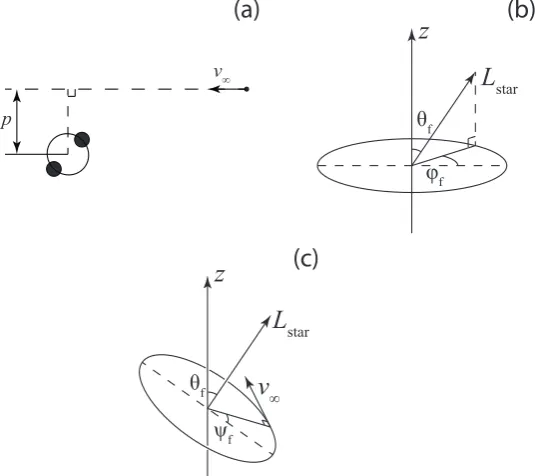
2.1 Orbital parameters of the massive binary. (a) Angular

mo-mentum Lbin, inclination θ, longitude of ascending node Ω,

argument of periapsis ω. The z axis coincides with the axis

of rotation of the nuclear cluster. (b) (θ, φ) is the direction

of the binary’s angular momentum vector in spherical coor-dinates; (Θ, ξ) or (Θ⊥,Θk) denote its change after a single interaction. . . 21

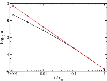
2.2 Notations for initial stellar orbital parameters used in this work. (a) Impact parameterpand velocity at infinityv∞. (b), (c) Other parameters of a star’s initial orbit: angular

momen-tumLstar, angles defining the direction of angular momentum

θf and ϕf (analogs of inclination and longitude of ascending

node, respectively, for an unbound orbit), angle defining the

direction of initial velocity in the orbital planeψf (analog of

argument of periapsis for an unbound orbit). . . 30

2.3 Left: shaded (blue) area corresponds to orbits in the

scat-tering experiments that would be bound to the galaxy given our adopted mapping (p, v∞) ⇔ (E, L), assuming γ = 5/2 and S = 6. Right: shaded area shows the region in (E, L)

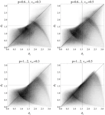
2.4 Black: number density of stars having (E, L) values that are representable via the scattering experiments. Red: total

num-ber density. This figure assumes a power-law density profile,

n∝r−5/2, and a binary hardnessS = 6. . . 39 2.5 Density plots showing the final angle, θf, between l and lbin

versus the initial angle,θi. Each frame contains results from

106 trajectories for different values ofp andv∞. . . 40 2.6 (a) Distribution of angular momentum changes for the stars

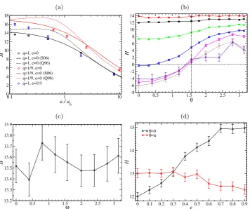
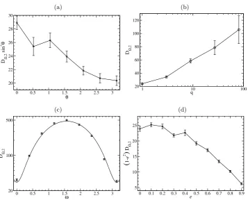
with p = 1. . .2, v∞ = 0.3. (b) Distribution of angular mo-mentum changes for the stars withp= 0.3, v∞= 1. . . 42 2.7 Dimensionless hardening rate H (Equation 2.72c) as a

func-tion of binary orbital elements and the parameters that define the stellar nucleus. (a) Dependence of H on binary hardness

a/ah (Equation 3.5) for a binary in a nonrotating nucleus.

Black is for q = 1, e = 0, red is for q = 9, e = 0, blue is for q = 1, e = 0.9. Symbols are the results of scattering

experiments, solid curves are Equation (16) of Sesana et al.

(2006), dashed curves are Equation (18) of Quinlan (1996). (b) Dependence of H on binary orbital inclination θ for a

circular, equal-mass binary in a maximally rotating (η = 1)

nucleus. Different colors are for S = 0.1,0.2,0.5,1,2,4,8 (a/ah = 1600,400,64,16,4,1,0.25), with higher S (lower

a/ah) corresponding to higher H(θ=π). (c) Dependence of

Hon the argument of periapsisωfor an equal-mass binary in a maximally-rotating nucleus, withS = 4,e= 0.5, θ=π/2.

(d) Dependence of H on binary eccentricity e for an

equal-mass binary in a maximally-rotating nucleus; S = 4. Black:

θ = 0; red: θ = π. The values of H are averaged over ω,

assuming a uniform distribution ofω. . . 47

2.8 Dimensionless diffusion coefficient in semimajor axisH0 (Equa-tion 2.72d) as a func(Equa-tion of binary orbital elements forq= 1,

η = 1. (a) Dependence of H0 on binary orbital inclination

θ for e= 0. (b) Dependence of H on binary eccentricity e.

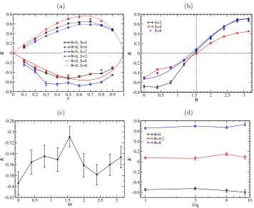
2.9 Dimensionless rate of change of eccentricityK(Equation 2.85c). Points: the dependence of K on various parameters for a

maximally-rotating nucleus (η = 1). Unless otherwise

indi-cated,q = 1, S = 4 (S= 8 on Fig. d), e= 0.5,θ=π/4. All of the figures show values of K averaged over ω assuming a

uniform distribution ofω. Curves: fits to Equation (2.86). . 52

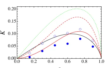
2.10 Eccentricity growth rate K for equal-mass binaries in non-rotating nuclei. Black line: our analytical approximation.

Green line: the results ofMikkola & Valtonen (1992) inS → ∞ limit. Red lines: the results ofQuinlan (1996) forS = 10

(solid) and S = 30 (dashed). Blue circles: the results of

Sesana et al.(2006) forS = 10 (filled) and S= 30 (empty). . 54

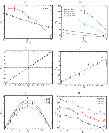
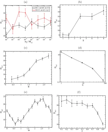
2.11 Dependence ofDθ,1andDθ,2 on various parameters:

semima-jor axis aexpressed in units ofah (defined in Equation 3.5),

degree of corotationη, binary inclinationθ, eccentricitye, bi-nary mass ratioq and argument of periapsis ω. If not stated

otherwise, S = 4, η = 1, e= 0 and q = 1 for both Dθ,1 and

Dθ,2,θ=π/2 for Dθ,1 and θ= 0 forDθ,2. . . 56

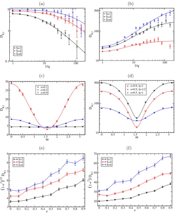
2.12 Continuation of Figure 2.11. The default parameter values

are the same except as follows: (b) η = 1/2; (d) θ = π/2,

e = 0.9; (f) θ = π/2. The lines on (a) and (b) are the an-alytical approximations given by Equation (2.90). The lines

on (c) and (d) are a0 +a1cos 2ω fits. (e) and (f) show the

values averaged over the argument of periapsis ω, assuming the uniform distribution of ω; note that these two figures

show√1−e2_D

θ,1and (1−e2)Dθ,1which have finite limits at

e→ 1, so Dθ,1 ∼ (1−e2)−1/2 and Dθ,2 ∼(1−e2)−1 in the

high-eccentricity limit. . . 57

2.13 Dependence ofDΩ,2on various parameters: binary inclination

θ, eccentricity e, mass ratio q and argument of periapsis ω. Unless otherwise stated, S = 4, η= 1, e= 0,q = 1 and θ=

π/2, except fore= 0.9 in (c). The line in (c) isa0+a1cos 2ω

fit. . . 62

2.14 Dependence ofDω,1 on various parameters. Unless otherwise

stated,mf/M12= 10−6,S= 4,η = 1,e= 0.8,q= 1,θ= 0.5.

2.15 Fraction of stars that ended up being captured by one of the (equal mass) black holes instead of escaping to infinity after

interacting with the binary. Capture radius was assumed to

ber0= 4rg = 4·GM_c2 . Black dots: v= 0.5vb,p= 0.6a..1a; red

dots: v= 200 km/s,p= 0..

√

2GM a

v (rp = 0..a); blue dots: the

same as red dots, but without relativistic terms in equations

of motion (that would correspond to tidal disruption instead of capture). Black and red lines correspond to κ = 3.1 and

κ= 4.5, whereκis the ratio of fraction of captured/disrupted stars tor0/a. . . 70

2.16 (a) Fraction of captured stars among the ones that have

ex-perienced n close interactions with the binary (or revolu-tions around the binary, measured as number of times when

drstar/dt= 0) for r0/(0.5a) = 0.005, v = 200 km/s; only the

values for odd n are shown, because even n already means that the star was captured. Horizontal line marks the overall

fraction of captured stars. (b) Total number of stars

cap-tured after n-th interaction; parameter values are the same as in Figure 2.16. . . 72

2.17 Distribution function f(θ, τ) sinθ for τ = 0,1,2,3,4,6 found

from numerical solution of Eq. (2.121) withα= 0.01; smaller mean values ofθ correspond to later times. The steady-state

distribution (f(θ, τ) at τ → ∞) is almost indistinguishable

from f(θ,6). . . 77 2.18 Upper panels show the time dependence of the mean (left) or

variance (right) of θ, computed numerically from Eq. (2.121)

(black) and analytically from Eq. (2.139) (red). Lower panels show the difference between numerical and analytic solutions. 78

2.19 Evolution of binary inclination θ for Dθ,1/H = 1/3 (solid

lines) and Dθ,1/H = 1 (dashed lines) with different initial

2.20 Evolution of orbital inclinationθand eccentricityeof a binary with M12 = 108M and q = 1 in a maximally corotating nucleus (η = 1), according to Equations (2.147) and (2.153).

Different line styles correspond to different initial values of

θ. The initial eccentricity is (a) 0.1, (b) 0.5, (c) 0.9. The

red curve separates the regimes where the hardening of the

binary is dominated by stellar encounters (to the left) and GW emission (to the right); its equation is a = aGR (see

Eq. 2.153). Note the use of a different scale for different plots. 84 2.21 The same as Figure 2.20 but for η= 0.8. . . 85

2.22 The same as Figure 2.20 but for η= 0.6. . . 86

2.23 The same as Figure 2.20 but for a nonrotating nucleus (η = 0.5) and initial eccentricities 0.1, 0.3, 0.5, 0.7 and 0.9. The

evolution ofθ is not shown because θ= const. . . 87

2.24 Contour plots ofeGR (Eq. 2.154) in the (e0, θ0) plane (initial

eccentricity and initial inclination at a/ah = 1) for M12 =

108M,q= 1 and four different corotation fractions. . . 87 2.25 Evolution of orbital inclinationθand eccentricityeof a binary

with M12 = 108M,q = 1,e0 = 0.5 and θ= 5π/6 at

differ-ent degrees of corotation, integrated using Equations (2.155)

and (2.156) for triaxial (dashed), axisymmetric (dotted) and spherical (dot-dashed) galaxies as well as in the full-loss-cone

approximation (solid). . . 90

2.26 Time dependence of orbital parameters of a binary withM12=

108M,q = 1,e0 = 0.5 and θ= 5π/6 at different degrees of

corotation, integrated using Equations (2.155) and (2.156) for

triaxial (dashed), axisymmetric (dotted) and spherical (dot-dashed) galaxies as well as in the full-loss-cone approximation

3.1 Fraction of the total GW strain atf = 1yr−1 contributed by massive binaries with (a) z < zmax, (b) M12 > M12,min, (c)

q > qmin or (d) M12 < M12,max. If not otherwise specified,

zmax = 4, qmin = 1/100, M12,min = 106M and M12,max =

1010M. Plots assume circular-orbit binaries and SBH-bulge mass ratio β = 0.001 (straight lines) or β = 0.003 (dashed

lines); for (a) and (c) both lines look identical. . . 105 3.2 Published estimates of the ratioMBH/Mgalaxy(orMBH/Mbulge)

ordered by publication date and SBH mass measurement method used. Every point corresponds to a single galaxy; mean

val-ues are indicated with horizontal ticks. Horizontal dashed

lines mark the values 0.003 (the currently accepted value) and 0.001 (the more conservative estimate considered in this

work). References: Magorrian et al. (1998), Merritt &

Fer-rarese (2001), Marconi & Hunt (2003), McConnell & Ma

(2013),Kormendy & Ho (2013),Reines & Volonteri (2015). . 111

3.3 Left: rotational properties of the galaxy models as a

func-tion of the parameter η. Filled and open circles show values measured at the galaxy half-mass radius and the SBH

influ-ence radius respectively, the line is Eq. (3.35). The

nonro-tating model from which the rononro-tating models were generated by orbit-flipping was described byDehnen(1993) density law

with γ = 1 and with an assumed SBH mass of 0.002Mgal.

Right: two distributions of η used in this work (see Eq.3.36 and 3.34). . . 114

3.4 Dimensionless eccentricity growth rateK(Eq. 3.47a) for

equal-mass binaries and varying eccentricity (left) or e = 0.9 and varying mass ratio (right) in nonrotating nuclei. Black curve

is our expression (3.48). Green dotted curve: the expression

of Mikkola & Valtonen (1992) in a → 0 limit. Red curves:

the results of Quinlan (1996) for a/ah = 0.16 (solid) and

3.5 Evolution of orbital inclination θ and eccentricity e for an equal-mass binary in a slowly-rotating nucleus (η= 0.6, left)

and (b) a maximally-rotating nucleus (η = 1, right),

com-puted using Eqs. (3.46) and (3.47) with M12 = 108M and

S = Sh. Different line styles correspond to different initial

values of θ. The initial eccentricity is always e0 = 0.5. The

red curve separates the regimes where the hardening of the bi-nary is dominated by stellar encounters (to the left) and GW

emission (to the right); its equation is a(e) = aGR,0F1/5(e)

(see Eq. 3.38a). . . 119

3.6 (a) Predicted GW strain for circular binaries. Black: our

model described in § 3.2 assuming the “triaxial” (efficient) hardening law and β = 0.003. Red: model from Sesana

(2013b). Blue: models from Ravi et al. (2014); solid lines

correspond to M12/M = 106.5...1011 and two different as-sumption about the stellar density profile; circles correspond

toM12/M = 106.5...1010. (b) Predicted GW strain for dif-ferent assumptions aboutβ(SBH mass) and binary hardening law. Black dot indicates the 95%-confidence upper limit from

PPTA (Shannon et al.,2015). . . 121

3.7 (a) Coalescence time (froma=ah toa≈0) as a function of

M12for equal-mass circular binaries in triaxial, axisymmetric

and spherical galaxies. (b) Coalescence time as a function

of q forM12 = 108M. (c) Strain amplitude (Eq. 3.50) for circular-orbit binaries in triaxial and axisymmetric galaxies

as a function ofβ (for spherical galaxiesAyr= 0). . . 122

3.8 Predicted GW strain for four different values of the nuclear corotation fraction η. All curves assume β = 0.001. Initial

orbital elements (e0, θ0) are assumed to be the same for all

binaries. . . 123 3.9 The dependence of strain amplitude for axisymmetric galaxy

3.10 Predicted GW strain assuming β = 10−3, “thermal” distri-butions of initial eccentricity, two different distridistri-butions of

θ0 (Eq. 3.31) and two different distributions of η (“low η”,

Eq. (3.34a); “highη”, Eq. (3.34b)) for (a) triaxial and (b) ax-isymmetric galaxies. Also shown for comparison is the curve

computed assuming a thermal eccentricity distribution and

no rotation (η= 1/2). . . 127 3.11 (a) Contribution of different galaxy types to the predicted

GW strain assuming β = 10−3 and zero eccentricity for all binaries. (b) Strain spectra including the mixture of galaxy

types described in the text, for different assumed distributions

of e0 and θ0. . . 127

4.1 A flowchart representation of the population synthesis

algo-rithm described in this chapter. . . 132

4.2 Comparison of the population synthesis method with the one presented in Chapter 3 for different initial BSBH parameters,

values of the SBH-bulge mass ratioβ and random realizations

of the model. Galaxies are assumed triaxial with the rotation parameter distribution as in Eq. (3.34a). In the left panel

e0= 0. . . 135

INTRODUCTION

In this dissertation I present a numerical model of the dynamical evolu-tion of a binary supermassive black hole (BSBH) in the stellar nucleus of a

galaxy (Chapter 2). One of the new features of the model is the inclusion

of galactic rotation which adds a new degree of freedom – the orientation of the BSBH orbit – and makes eccentricity evolution more complex.

The model is then applied to the calculation of the stochastic gravita-tional wave (GW) background generated by an evolving, cosmological

pop-ulation of BSBHs (Chapter 3). The GW background spectra are calculated

under different assumptions about the initial orbital elements of the BSBHs; galactic morphology; and SBH-galaxy scaling relations.

Finally, in Chapter 4 I describe a “population synthesis” method that

is based on the model for BSBH dynamics described in Chapter 2 and the distribution of galaxy and BSBH parameters used in Chapter 3. The work

described in Chapter 4 was carried out as part of my collaboration with the

NANOGrav1 group. The output of the population synthesis code is going to be used in the analysis accompanying their 11-year data release (to come

out in 2017). Comparison of the numerically generated strain spectra with

observational pulsar timing array (PTA) constraints on the GW background level will allow us to place constraints on the parameters that define the

distribution of BSBHs.

The current chapter presents the background information that is

sary to place my work in the broader context of modern astrophysics and cosmology. In Section 1.1, I outline the theoretical arguments and the

ob-servational evidence in favor of the existence of BSBHs. In Section 1.2, I

describe the dynamical evolution of BSBHs in the stellar nuclei of galaxies and present an overview of previous results on that subject. Section 1.3

then discusses the GW emission from BSBHs, focusing on the stochastic

background and the prospects of its detection by means of pulsar timing data. Section 1.4 gives the chapter synopsis.

1.1

Binary supermassive black holes

According to the current cosmological paradigm, galaxies are surrounded

by extensive dark matter halos, and galaxies can grow in size when they

come close enough to other galaxies for the dark matter to induce a merger

(Mo et al.,2010). Many galaxies are also known to contain a supermassive

black hole (SBH) at their center, and it is commonly assumed that SBHs are

universally present in early-type galaxies, and in the bulges of disk galaxies, at least for galaxies above a certain mass (Merritt,2013, Chapter 1). Taken

together, these two hypotheses imply the formation of binary SBHs. The

idea was pioneered by Begelman et al.(1980), who suggested that both of the SBHs would lose energy due to interaction with the galactic environment

(stars and/or gas) until they become gravitationally bound to each other and eventually start losing energy due to GW emission and coalesce. All

these mechanisms of BSBH orbital evolution are analyzed in more detail in

Sections 1.2 and 1.3.

If the merging galaxies are gas rich, it is possible that at least one of the

two SBHs will accrete significant amounts of gas and will become an active

galactic nucleus (AGN). In those cases, it is possible to distinguish a binary from a single SBH by means of electromagnetic observations. The most

convincing detection method is direct imaging of a dual or displaced AGN

(if both or just one SBH is active, respectively). This technique requires a high enough angular resolution, which is why only one of the dual/displaced

AGN detected so far has a separation of 7.3 pc (Rodriguez et al.,2006) with

all the others being at least two orders of magnitude wider (Barth et al.,

merger.

The detection of SBH pairs with parsec-scale separations, which in most cases cannot be resolved, requires the use of different techniques. One of

them is periodic variability in AGN luminosity on a timescale associated

with the orbital period of the binary. As was shown in hydrodynamical sim-ulations (e.g.Noble et al.,2012), BSBHs carve a cavity in the accretion disc

and the gas flows from the inner edge of the accretion disc onto the binary

in a periodic fashion. More than a hundred of such BSBH candidates have been found already (Charisi et al., 2016; Graham et al., 2015). The most

well-studied of them is the quasar OJ 287 (Valtonen et al.,2008) which has

the first photometric measurements dating back to 19th century. However, it has been argued that unless most of the aforementioned candidates are false

positives, such a large number of BSBHs is inconsistent with the current upper limits on the stochastic GW background (Sesana et al.,2017).

Another BSBH observational signature is periodic variation of the AGN

spectrum, namely the offset of broad emission lines with respect to the narrow emission lines (Ju et al., 2013; Runnoe et al., 2017; Wang et al.,

2017). The former are generated by the gas bound to the SBHs whereas

the latter are generated by the gas in the galaxy far from the BSBH, so the periodic Doppler shift of broad lines is due to the orbital motion of SBHs

around each other. However, for very compact BSBHs the broad lines might

in fact be generated within the circumbinary disk, making this interpretation problematic.

There is also the following indirect evidence of past or ongoing BSBH

formation in massive elliptical galaxies: the presence of low-density cores, or “mass deficits” (Merritt, 2013, §2.1). Mass deficits arise due the “gravita-tional slingshot” mechanism (see Section 1.2 for more detail) when a BSBH

effectively ejects the stars from the galactic center with high velocities. Finally, a possible observable consequence of BSBH mergers is emission

of gravitational waves (GWs). Compared with the GWs detected by LIGO

from stellar-mass BHs, the GWs produced during the late evolution of BS-BHs would have much lower frequencies and thus require different sorts of

equipment to detect. So far two different techniques have been proposed:

(1) space-based laser interferometers (LISA, ALIA, DECIGO) and (2) pul-sar timing arrays (PTAs). The latter are used to carry out decades-long

subtle effects of the passage of gravitational waves through the intervening

space. Space-based interferometers are still in the development stage; PTAs (e.g. NANOGrav, EPTA, PPTA) are currently active, but have so far only

established upper limits on the intensity of the GW background radiation.

See Section 1.3 for a detailed discussion.

1.2

Dynamical evolution

Begelman et al.(1980), who first suggested the concept of BSBHs, broke

down the likely evolution of a massive binary into three stages:

1. In the early phases of the galaxy merger, the two SBHs are far enough

apart that they move independently in the potential of the merger remnant. Both SBHs sink toward the center of the potential due to

dynamical friction against the stars.

2. When they are close enough together – roughly speaking, within their

mutual spheres of gravitational influence – the two SBHs form a bound pair. Their two-body orbit continues to shrink due to exchange of

energy and angular momentum with nearby matter: through

gravita-tional slingshot interactions with stars, or gravitagravita-tional torques from gas.

3. If the binary separation manages to shrink to a small fraction of a

parsec, emission of gravitational waves brings the two SBHs even closer

together, resulting ultimately in coalescence.

I now briefly describe these three phases of evolution in more detail.

1.2.1 Dynamical friction

When a massive object moves through a field of stars, a region of over-density is formed behind it, which exerts an extra gravitational force and

slows it down (Chandrasekhar,1943). This extra force is called “dynamical

friction”. A standard expression, due to S. Chandrasekhar, for the dynami-cal friction force is

dυυυ ₂υυυ Z υ

wherem? is the stellar mass,mis the mass of the massive object,vits

veloc-ity, ln Λ the Coulomb logarithm, and f(v?) the stellar velocity distribution

function. We see that deceleration due to that force is proportional to the

mass of the object, which is why it is an effective energy loss mechanism for

a SBH. Applied to the case of a BH spiraling toward the center of a spherical galaxy on a circular orbit,2 this formula gives an inspiral timescale of the

order of 10 Gyr (Binney & Tremaine,1987, Eq. 8.12):

TDF≈

19 ln Λ

Re

5kpc

2

σ

200km s−1

108M

m

Gyr (1.2)

where Re and σ are the galaxy’s effective radius and velocity dispersion,

and m is the BH’s mass. However, the preceding equation assumes the

BH to be “naked”, while in reality a SBH brought in during the course of a galaxy merger would retain a fraction of its host galaxy’s stellar bulge,

increasing its effective mass. Considering that the mass of a central bulge is about 103_M

BH (McConnell & Ma, 2013; Merritt & Ferrarese, 2001), it

follows that the actual inspiral time could be up to three orders of magnitude

shorter. Given a realistic estimate of a galaxy mass fraction that would be tidally stripped, the resultant timescale is shorter than 1 Gyr (Dosopoulou

& Antonini, 2017) as long as the mass ratio of the two SBHs is not too

extreme (&10−2).

1.2.2 Stellar ejections

As the two SBHs spiral toward the center of the galaxy, eventually they

come close enough together that they form a bound pair. This occurs,

roughly, when the mass in stars interior to the binary’s orbit is less than the binary’s mass. Once this happens, a new dynamical mechanism comes

into play: slingshot ejection of stars. Whenever a star approaches within a

few orbital separations of the binary, it experiences a strong, and strongly time-dependent, gravitational interaction with the SBHs. That interaction

sometimes ends with the star getting captured on a stable orbit around one of the SBHs, but in the vast majority of cases the star gets ejected away

from the binary, carrying a small part of the binary’s energy and angular

momentum with it. As a consequence, the binary continues to shrink. Slingshot ejections continue until the supply of stars is depleted. That

2

may never happen; but at least in a spherical galaxy, the number of stars on

orbits that intersect the binary is expected to drop suddenly when the binary becomes “hard”, i.e. when its semimajor axis falls below the “hard-binary

separation”ah:

ah =

GM1M2/(M1+M2)

4σ2 (1.3)

whereσ is stellar velocity dispersion in the galaxy center (Merritt,2013, Eq.

8.23). Whena < ah, stars are ejected with high enough velocities to escape

completely from the nucleus. The result would be a rapid depletion of the supply of interacting stars, and binary evolution would cease: the evolution

would “stall.”

In addition to changing the semimajor axis (i.e. binding energy) of the binary, slingshot interactions cause changes in the other binary orbital

ele-ments as well. To calculate the rate of change of a BSBH orbital eleele-ments, a technique called “scattering experiments” is usually employed: a three-body

interaction between the two SBHs and a star approaching them is simulated

until the star becomes unbound from the BSBH (is ejected with velocity large enough to escape from the BSBH to infinity), and that simulation is repeated a large number of times (∼105) with the parameters of the stellar

orbit (initial velocity, impact parameter etc.) chosen randomly every time. At the end of every simulation the changes in the BSBH orbital parameters

are recorded, and after enough simulations are made to cover all stellar

or-bit parameter space, that change is averaged over all simulations and then converted into an average rate of change.

In the simplest case of a circular BSBH placed in an isotropic and

uni-form stellar background, there is only one orbital parameter of importance: the orbital separation or semimajor axis a. It has been shown in different

scattering experiment studies (Mikkola & Valtonen, 1992; Quinlan, 1996;

Sesana et al.,2006) that for hard binaries the “hardening rate” is

d dt

1

a

= HGρ

σ , H ≈15, (1.4)

whereρandσ are stellar density and velocity dispersion. The characteristic

stellar hardening timescale is

It becomes longer as the binary shrinks because its effective “capture radius”

for close stellar interactions (which is proportional to a) is decreasing, i.e. less stars approach the binary close enough to contribute to its hardening.

If the BSBH eccentricity is nonzero, it is affected by stellar ejections as

well. In the studies cited above, eccentricity was shown to increase signifi-cantly for hard binaries in isotropic stellar backgrounds, although different

papers give somewhat different estimates of its rate of change.3 As for the

orientation of a BSBH orbit, it experiences a small random walk akin to Brownian motion due to the random and discrete nature of stellar

interac-tions (Merritt,2002).

However, some recent studies have shown that the situation becomes qualitatively different if we consider a massive binary in a rotating stellar

nucleus (a nucleus with nonzero total angular momentum). The eccentricity evolution then depends on the mutual orientation of the BSBH orbit and the

axis of nuclear rotation: the eccentricity tends to decrease if the BSBH is

corotating (i.e. has angular momentum in the same direction as that of the stellar nucleus) and tends to increase if the BSBH is counterrotating (Sesana

et al.,2011). The orientation of the binary’s orbital plane also evolves: the

binary tends to become corotating, i.e. its angular momentum vector aligns in direction with the stellar angular momentum vector(Gualandris et al.,

2012;Wang et al.,2014). Cui & Yu(2014) have shown that a similar effect

takes place if the stellar nucleus is flattened (axisymmetric).

1.2.3 The effects of gas

During galaxy mergers, gas, if present, can be driven by torques and

dynamical instabilities to the center of the merger remnant (Mihos &

Hern-quist,1996), interacting with the SBHs. In the early stages of BSBH

evo-lution, large amounts of gas can significantly increase the dynamical

fric-tion (Escala et al., 2005). After the hard binary formation, a rotationally supported gas disk might form around the binary. The binary excites

non-axisymmetric perturbations in the disk which exert a torque on the binary

reducing its energy and angular momentum (Haiman et al., 2009). Unlike stellar hardening, the characteristic timescale for this effect decreases as the

binary shrinks: thard ∼aγ, γ >0, where the exact value ofγ depends on the

3

de/dtis more computationally difficult to calculate thanda/dtbecause the eccentricity

binary and disk parameters. This makes the presence of an accretion disk a

promising mechanism for overcoming the “final parsec problem” (§1.2.5). The accretion disk also influences BSBH eccentricity depending on their

mutual orientation, similarly to a rotating stellar nucleus (§1.2.2): corotating gas disks decrease the BSBH eccentricity and counterrotating ones increase

it (Dotti et al.,2006;Schnittman & Krolik,2015). If the gas disk is initially

misaligned with respect to the BSBH orbital plane (such a configuration can

occur from the infall and subsequent circularization of gas into the inner few parsecs of the merger remnant), it tends to align with it, becoming

either co- or counterrotating. If the binary is eccentric, polar alignment can

also occur, when the disk angular momentum is aligned with the binary periapsis or apoapsis direction (Aly et al.,2015). Such polar disks are prone

to disruption with subsequent gas infall onto the binary, which is then ejected via gravitational slingshot, hardening the binary.

1.2.4 Gravitational wave emission

In addition to changes due to interaction with its nuclear environment,

BSBH orbital parameters can also change due to the effects of general rel-ativity (GR). In particular, the emission of gravitational waves results in

the binary losing energy (which decreasesa) and causes its orbit to become

more circular:

da dt

GR

= −64 5

νG3M₁₂3

c5_a3 f(e), (1.6a)

de dt

GR

= −304 15

νG3M₁₂3

c5_a4 g(e), (1.6b)

M12 = M1+M2, ν =

M1M2

(M1+M2)2

, (1.6c)

f(e) = 1 + (73/24)e

2_{+ (37/96)e}4

(1−e2₎7/2 , (1.6d)

g(e) = e1 + (121/304)e

2

(1−e2₎5/2 . (1.6e)

It is easy to see from these equations that effects of GW emission have a very

steep dependence ona. As a result, they are insignificant at the early stages

of a BSBH dynamical evolution, but at a certain orbital separationaGRthey

is approximately the time it takes the binary to reach aGR. The orbital

shrinking is enhanced for eccentric binaries (the f(e) factor), so the GR-dominated regime starts earlier for them. Then the eccentricity decreases

quickly, so the SBHs enter the final stages of coalescence on almost circular

orbits.

1.2.5 The “final parsec problem”

A shortcoming of the scattering experiments method is that it assumes

an unchanging distribution of stars in the nucleus, while in reality, evolu-tion of a massive binary is likely to be accompanied by changes in the stellar

density: the stars that get ejected from the galactic center are unlikely to

interact with the binary again. The orbits of the ejected stars can be re-populated because of the process called “relaxation”: random fluctuations

in stellar orbital parameters due to either occasional close gravitational

in-teractions with other stars or massive perturbers (“collisional relaxation”) or non-sphericity of the galactic potential (“collisionless relaxation”). This

way, the hardening rate depends on the repopulation rate of the orbits

ap-proaching the pericenter closer than∼a(“loss cone”) as much as onρandσ. And if this repopulation is not fast enough, the BSBH might stall ata > aGR

for more than a Hubble time, never reaching coalescence. This phenomenon

is known as the “final parsec problem” (Milosavljevi´c & Merritt,2003). How strong this effect is likely to be in real galaxies has been a subject

of debate. One way to find out is to perform a numerical simulation that

includes all the stars of the galaxy (an N-body simulation). In practice, the number of stars in a real galaxy (&109) would be too high for such a simulation to be computationally feasible, so what people do instead is a simulation in which every particle represents a large number of stars (e.g.

103). Because the timescale for collisional relaxation scales as ∼ N (given

fixed, total mass in stars), these simulations have difficulty moving out of the collisional regime, and it is difficult to scale the results so obtained to the

regime of largerN. While all studies agree that the final parsec problem does

indeed exist in spherically symmetric galaxies where collisional relaxation is absent (stellar energy and angular momentum are conserved in spherical

potentials), different N-body models give contradicting results on whether

it is solved in axisymmetric or triaxial galaxies with finite N (Khan et al.,

A numerical technique that attempts to remove this drawback ofN-body

simulations was developed by Vasiliev et al. (2014, 2015): a Monte-Carlo method where all the stars are assumed to be moving in a smooth potential,

and random fluctuations imitating collisional relaxation are periodically

ap-plied to the orbital parameters. These authors conclude that axisymmetry is not enough to make the SBHs coalesce in less than a Hubbe time, but even

a modest degree of triaxiality (e.g. 1:0.9:0.8) implies coalescence timescales

.1 Gyr. Vasiliev et al. have also derived analytical approximations for the hardening rate in galaxies of different geometry which I use in my model of

BSBH dynamics as a correction to the results of scattering experiments.

1.3

Gravitational wave emission from BSBHs and

its detection prospects

As discussed above, the emission of gravitational waves (GWs) will dom-inate the evolution of a BSBH if its orbital separation is small enough. As

of this writing, no detection has been made of GWs from supermassive

bi-naries, even though GWs from stellar-mass binary black holes have been detected by the LIGO collaboration (Abbott et al.,2016). Part of the

rea-son is that GWs from BSBHs typically have much lower frequency. The

fre-quency of the emitted GW is determined by the binary’s orbital frefre-quency

forb: the radiation is monochromatic (f = 2forb) for circular binaries, and

eccentric binaries radiate at a discrete spectrum of frequencies: fn=nforb,

n= 1,2,3, . . ., with

forb=

1 2π

r

GM12

a3 = 3.4×10

−12

M12

108_M

1/2

a

1 pc

−3/2

Hz, (1.7)

whereM12 is the total BSBH mass andais its semimajor axis. Because of

the low frequencies, detection of GWs from BSBHs requires techniques

dif-ferent from LIGO’s ground-baser laser interferometry. One such techniques is pulsar timing. Millisecond pulsars, with their highly periodic radio

emis-sion, provide an opportunity to detect space-time perturbations caused by

a GW passing between the pulsar and the Earth. A set of pulsars is chosen and the moments of arrival of its pulses are recorded by an array of radio

the pulses – the timing residuals – carry information about the GWs, and

this information is extracted by cross-correlating residuals between different pulsars (Hellings & Downs, 1983). There are, however, many other

possi-ble sources of non-periodicity in the pulse arrival times, such as pulsar spin

instability, fluctuations in pulsar magnetospheres, dispersion and scattering in the interstellar plasma etc., which makes the extraction of a GW

sig-nal a very challenging problem (Cordes, 2013; Cordes et al., 2016; Lentati

et al., 2016). The frequency range that PTAs can probe is limited by the

observation time to f & 1/T, with T the total time of observation. The frequency of greatest sensitivity is of order of that minimal frequency.

Cur-rent PTA groups include the European PTA (EPTA), the North American Nanohertz Observatory for Gravitational Waves (NANOGrav), the Parkes

PTA, and the International PTA (IPTA), the latter being the union of the former three. All of these groups have been collecting data forT ≈10 yr.

The PTA method can be used to detect both GWs from a single BSBH

(“continuous GWs”) and the local superposition of GWs from all the BSBHs in the universe (“GW background”). The detection of the former opens an

interesting possibility for multimessenger observations of BSBHs, combining

GWs and conventional electromagnetic observations (Burke-Spolaor,2013). However, it is considered much less likely to happen in the next few years

compared to the GW background detection (Rosado et al.,2015), which is

why the latter is the main focus of most PTA studies.

The measure of GW background intensity is its characteristic strain4 hc,

a measure of its energy density per unit frequency (Phinney,2001):

hc(f) =

4G πf

dρGW

df . (1.8)

The exact value of hc(f) is defined by the time binaries spend radiating

at the frequency f – in other words, by their dynamical evolution. In the simplest case of circular-orbit binaries that are evolving solely due to GW

emission (Eqs. 1.6), the resultant spectrum is

hc(f) =Ayr

f fyr

−2/3

(1.9)

4

where fyr ≡ 1/yr. This expression was derived in the assumption of a

large number of binaries, radiating at a randomly distributed points in their lifetime (which is what we would expect from the BSBHs in the universe);

a small number of binaries would produce a more discrete spectrum, as was

mentioned earlier. If we take environmental effects (interaction with stars or gas) into account, the value of hc will be decreased at low frequencies,

since those effects accelerate the evolution of the binary’s orbit at high a

(i.e. lowforb). Sampson et al.(2015) suggested a simple parametrization of

the strain spectrum for a population of environmentally influenced binaries:

hc(f) = A

(f /fyr)−2/3

[1 + (fbend/f)κ]1/2

, (1.10a)

A = Ayr[1 + (fbend/fyr)κ]1/2 (1.10b)

wherefbend is understood as the orbital frequency below which

environmen-tal interactions dominate the binary’s evolution andκ is determined by the

type of interaction; in the case of stellar scattering in a full loss-cone regime,

κ = 10/3. Simple evolutionary models suggest fbend ≈ 10−9 Hz (Sesana,

2013b), a frequency regime that is beginning to be probed by PTAs. Nonzero

eccentricity also changes the shape of the spectrum, decreasinghcatf .forb

(Ravi et al.,2014).

It is difficult to make definite theoretical estimates ofAyrsince it depends

on many uncertain factors: the galaxy merger rate, the SBH-galaxy scaling relations, the strength of environmental effects, the eccentricity distribution

of BSBHs at their time of formation etc. (Chen et al., 2016; McWilliams

et al.,2014;Ravi et al.,2014; Sesana et al.,2016;Sesana,2013a; Simon &

Burke-Spolaor,2016). The predictions of the cited studies range from 10−16

to 10−14 at f = fyr. The current observational upper limits on Ayr are

3.0×10−15 (EPTA, Lentati et al., 2015); 1.0×10−15 (PPTA, Shannon et al.,2015); and 1.5×10−15 (NANOGrav, Arzoumanian et al., 2016), which is already low enough to rule out some of the models.

There is another possible class of instruments for low-frequency GW de-tection which hopefully will become available in the future: space-based laser

around 2030.5 The proposed configuration is a constellation of three

space-craft, arranged in an equilateral triangle with sides 2.5 million km long, on a heliocentric orbit trailing the Earth. The distance between the satellites will

be precisely monitored by means of laser interferometry to detect a passing

gravitational wave. Such a telescope would be sensitive to frequencies above 10−4 Hz, which would allow it to detect BSBH mergers as well as extreme mass-ratio inspirals and the early evolution of stellar-mass BHs.

In principle, it is possible to detect the same individual BSBH using both PTA and SLI: a BSBH can be tracked by PTA first and them by

SLI during merger and ring-down (Pitkin et al., 2008). Alternatively, SLI

can detect a BSBH first and place constraints on its parameters, and these constraints can provide information on where to search for its signal at the

earlier evolution stages in the PTA data. However, the possibility of such complimentary detections is estimated to be rather low (Spallicci,2013).

1.4

Chapter synopsis

In this dissertation I present the results of two numerical studies on the dynamics of BSBHs in rotating galactic nuclei and its impact on the

nanohertz GW background. This work aims to construct more realistic

models of both BSBH dynamics and GW background as most of the galaxies possess some degree of rotation.

In Chapter 2, I present the results of the scattering experiments

per-formed in the assumption of anisotropic distribution of stellar angular mo-menta (i.e. nonzero rotation). I calculate first- and second-order diffusion

coefficients for all the BSBH orbital components and find their dependence on the degree of stellar rotation. I then derive the differential equations

that describe the time evolution of BSBH orbital parameters for given

ini-tial conditions and galaxy parameters.

These equation are then used in Chapters 3 and 4 to calculate the strain

spectrum of GW background in different assumptions about BSBH and

galaxy parameter distribution. Apart from BSBH dynamics, the impact of other factors is discussed, such as SBH-galaxy scaling relations and galaxy

merger rate. As those are not very well observationally constrained, its

important to understand how varying them affects the GW background

tensity and which values of those parameters are allowed by the current PTA

constraints.

Chapter 5 summarizes the results of my work and their implications for

DYNAMICAL EVOLUTION OF A BSBH IN A

ROTATING STELLAR NUCLEUS

2.1

Introduction

According to the current paradigm, galaxies are surrounded by extensive

dark matter halos, and galaxies can grow in size when they come close

enough to other galaxies for the dark matter to induce a merger (Mo et al., 2010). Many galaxies are also known to contain a supermassive black

hole (SBH) at their center, and it is commonly assumed that SBHs are

universally present in early-type galaxies, and in the bulges of disk galaxies, at least for galaxies above a certain mass (Merritt,2013). Taken together,

these two hypotheses imply the formation of binary SBHs. The idea was

first explored byBegelman et al.(1980), who broke down the likely evolution of a massive binary into three stages:

1. In the early phases of the galaxy merger, the two SBHs are far enough

apart that they move independently in the potential of the merger remnant. Both SBHs sink toward the center of the potential due to

dynamical friction against the stars.

2. When they are close enough together – roughly speaking, within their

mutual spheres of gravitational influence – the two SBHs form a bound pair. Their two-body orbit continues to shrink due to exchange of

gravita-tional slingshot interactions with stars, or gravitagravita-tional torques from

gas.

3. If the binary separation manages to shrink to a small fraction of a parsec, emission of gravitational waves brings the two SBHs even closer

together, resulting ultimately in coalescence.

The present chapter focusses on the second of these three phases. Fur-thermore, only interactions of the massive binary with stars are considered;

gaseous torques are ignored. In certain respects, this is well-trodden ground.

Using numerical scattering experiments,Mikkola & Valtonen(1992), Quin-lan (1996) and Sesana et al. (2006) derived expressions for the rates of

change of binary semimajor axis and eccentricity, for binaries in spherical

nonrotating nuclei. Merritt (2002) noted that the same interactions would induce changes also in the other elements of the binary’s orbit – for instance,

its inclination – and he obtained expressions for the rate of change of a

bi-nary’s orientation from scattering experiments. If the nucleus is spherical and nonrotating, these changes take the form of a random walk, similar in

many ways to the “rotational Brownian motion” of a polar molecule that collides with other molecules in a dielectric material (Debye,1929). In both

cases, evolution can be described via a Fokker-Planck equation in which the

independent variable is a quantity (angle) that defines the orientation: the orbital plane in the case of a massive binary, the dipole moment in the case

of a molecule.

N-body simulations of galaxy mergers suggest that the stellar nuclei of merged galaxies should be flattened and rotating (e.g.Gualandris & Merritt,

2012;Milosavljevi´c & Merritt,2001). Since there is a preferred axis in such

nuclei, it would not be surprising if the orbital plane of a massive binary evolved in a qualitatively different manner, due to slingshot interactions, as

compared with binaries in spherical and nonrotating nuclei. RecentN-body

work has addressed this possibility (Cui & Yu,2014;Gualandris et al.,2012;

Wang et al., 2014). One finds in fact that the orbital angular momentum

vector of the binary tends to align with the rotation axis of the nucleus.

There are corresponding changes in the evolution of the binary’s eccentricity

(Sesana et al.,2011). Stellar encounters tend to circularize the binary if its

In the present chapter, we return to a Fokker-Planck description of the

evolution of a massive binary at the center of a galaxy. As inMerritt(2002), we use scattering experiments to extract the diffusion coefficients that

ap-pear in the Fokker-Planck equation. However we generalize the treatment in

that paper in a number of ways. (i) InMerritt (2002) (as inDebye(1929)), a single diffusion coefficient described changes in the orbital inclination, and

this coefficient was assumed to be independent both of the binary’s

instan-taneous orientation and of the direction of its change. In the present work, those assumptions are relaxed, allowing us to describe orientation changes

in the general case of a binary evolving in an anisotropic (rotating)

stel-lar background. (ii) Both first and second-order diffusion coefficients are calculated; the former are most important in the case of rapidly rotating

nuclei, the latter in the case of slowly rotating nuclei. (iii) Terms describing the rate of change of binary separation and eccentricity due to gravitational

wave emission are included; in this respect, our work carries the evolution

of the binary into the third of the three phases defined byBegelman et al.

(1980).

A shortcoming of this approach is that the scattering experiments

as-sume an unchanging distribution of stars in the nucleus, while in reality, evolution of a massive binary is likely to be accompanied by changes in the

stellar density. Exactly how these two sorts of evolution are coupled has

been debated in the past. At one extreme, it is possible for the binary to “empty the loss cone” corresponding to orbits that pass near the binary. If

this happened, the density of stars in the vicinity of the binary would drop

drastically, and the binary would cease to harden; or it would harden at a rate determined by collisional orbit repopulation, which is very slow in all

but the smallest galaxies. The possibility that binaries “stall” at

parsec-scale separations was considered likely by Begelman et al. (1980), and the term “final-parsec problem” was coined byMilosavljevi´c & Merritt(2003) to

describe the difficulty of evolving a binary past this point. However, recent

work (Gualandris et al.,2017;Khan et al.,2013;Vasiliev et al.,2014,2015) has made a strong case that massive binaries typically do not stall in this

way. Rather, one finds that even slight departures of a nucleus from spherical

symmetry allow stars to be continually fed to a central binary, at rates that decrease slowly with time, but which can be much greater than rates due to

con-sidering that the product of a galactic merger is expected to be generically

triaxial (Gualandris & Merritt, 2012; Khan et al., 2016). We incorporate the results of this work, and in particular the study ofVasiliev et al.(2015),

into our evolution equations, and thus account in an approximate way for

the back-reaction of the binary’s evolution on its stellar surroundings. This chapter is organized as follows. In §2.2 we generalize the Fokker-Planck formalism used byDebye(1929) andMerritt(2002) to include changes

in all the elements of a binary’s orbit, in a stellar nucleus that has an axis of rotational symmetry. §2.3 describes the scattering experiments and the method for extracting diffusion coefficients. In§2.4 we present a qualitative analysis of the results of the scattering experiments and try to explain some of their phenomenology. In§2.6 we estimate the influence of post-Newtonian effects. §2.5 presents the results of numerical calculation of diffusion coeffi-cients for all the orbital components of the binary. Finally, in §2.8 we use these results to solve the FPE for the distribution function of binary’s orbital

inclination. §2.9 sums up and discusses some observational implications of our results.

An important application of the results obtained here is to calculations

of the stochastic gravitational wave spectrum produced by a cosmological population of massive binaries in merging galaxies. This is the subject of

Chapter 3.

2.2

Equations of binary evolution

Consider a massive binary at the center of a galaxy. The components of

the binary have masses M1 and M2, which are assumed to be unchanging,

and M1 ≥ M2. If the binary is treated as an isolated system, its energy

Ebin and angular momentum Lbin are related to its semimajor axis a and

eccentricity evia

Ebin=−µ

GM12

2a , Lbin=µ

p

GM12a(1−e2) (2.1)

whereM12=M1+M2is the binary’s total mass andµ=M1M2/(M1+M2)

its reduced mass. For the remainder of this section, we will useE ≡Ebin/µ

momen-tum, respectively, of the massive binary:

E=−GM12

2a , L=

p

GM12a(1−e2). (2.2)

Five variables are needed to completely specify the shape and orientation

of the binary’s orbit. Four of these can be taken to be (E,L); the fifth

variable determines the orientation of the major axis of the binary’s orbit (in the plane determined by the direction ofL) and is usually taken to beω,

the argument of periapsis. BothEandLare independent ofω. In principle,

one could evaluate changes in ω due to interaction of the binary with stars using the numerical scattering experiments described below. We choose

to ignore changes in ω in our Fokker-Planck description of the binary’s

evolution. That is a valid approximation in two limiting cases: when ω

does not change at all; or when ω changes so rapidly that we can average

all the other diffusion coefficients over ω. In §2.5.5 we show the latter to be a good approximation for a wide range of possible system parameters. Accordingly, in much of what follows, our expressions for quantities like the

diffusion coefficients in E and L will be averaged overω.

2.2.1 Fokker-Planck equation

The binary is assumed to interact with stars, causing changes in its

orbital elements.1 In the simplest representation, the binary’s orbit would

evolve smoothly and deterministically with respect to time. We consider a slightly more complex model, in which a random, or diffusive, component

to the binary’s evolution is allowed as well.

Accordingly, define f(E,L, t)dE dL to be the probability that the bi-nary’s energyE and angular momentumLlie in the intervalsE toE+dE

and L to L+dL, respectively, at time t. Let ∆t denote an interval of

time that is short compared with the time over which the orbit of the bi-nary changes due to encounters with stars, but still long enough that many

encounters occur. Define the transition probability Ψ(E,L; ∆E,∆L) that

the energy and angular momentum of the binary change by ∆E and ∆L,

1_{Changes in the location of the binary’s center of mass are ignored; these were discussed}

respectively, in time ∆t. Then

f(E,L, t+ ∆t) =

Z

f(E−∆E,L−∆L, t)

× Ψ (E−∆E,L−∆L; ∆E,∆L)dEd∆L. (2.3)

This equation assumes in addition that the evolution off depends only on its instantaneous value, that is, that its previous history can be ignored

(“Markov process”).

We now expand f(E,L, t+ ∆t) on the left-hand side of Equation (2.3) as a Taylor series in ∆t, and f(E−∆E,L−∆L, t) and

Ψ (E−∆E,L−∆L; ∆E,∆L) on the right-hand side as Taylor series in ∆E and ∆L. Retaining only terms up to second order, the result is

∂f

∂t = −

∂ ∂Lx

(fh∆Lxi)−

∂ ∂Ly

(fh∆Lyi)−

∂ ∂Lz

(fh∆Lzi)−

∂

∂E(fh∆Ei)

+ 1 2

∂2 ∂L2

x

fh∆L2_xi

+1 2

∂2 ∂L2

y

fh(∆Ly)2i

+1 2 ∂2 ∂L2 z

fh(∆Lz)2i

+ 1 2

∂2

∂E2 fh(∆E) 2_i

+ ∂

2

∂Lx∂Ly

(fh∆Lx∆Lyi)

+ ∂

2

∂Lx∂Lz

(fh∆Lx∆Lzi) +

∂2

∂Ly∂Lz

(fh∆Ly∆Lzi)

+ ∂

2

∂Lx∂E

(fh∆Lx∆Ei) +

∂2

∂Ly∂E

(fh∆Ly∆Ei)

+ ∂

2

∂Lz∂E

(fh∆Lz∆Ei). (2.4)

Diffusion coefficients are defined in the usual way as

h∆xi = 1

∆t

Z

Ψ(E,L; ∆E,∆L) ∆x d∆E d∆L,

h∆x∆yi = 1

∆t

Z

Ψ(E,L; ∆E,∆L) ∆x∆y d∆Ed∆L, (2.5)

where{x, y} can be any of {Lx, Ly, Lz, E}.

We will often be interested in the case of a binary that evolves in a

ro-tating stellar nucleus. Suppose that the nucleus is unchanging and spherical

and that the center of mass of the binary coincides with that of the nuclear star cluster. Assume furthermore that the total angular momentum with

di-angular momentum vector may be inclined with respect to this axis, by an

angleθ(t). In this case it is useful to express the Fokker-Planck equation in terms of angular momentum variables for the binary that are defined with

respect to thez-axis, for instance

x1 =L, x2 =µ= cosθ=Lz/L, x3=φ, x4 =E. (2.6)

With the right choice of “reference axis” and “reference plane,”θ is

equiv-alent to the orbital inclination of the binary, usually denoted byi, and φis equivalent to the longitude of its ascending node, or Ω (Figure 2.1a).

Θ_║

Θ┴ Θ ξ θ

φ

(a)

(b)

z

L

bin

x

ω

Ω θ

Figure 2.1: Orbital parameters of the massive binary. (a) Angular momen-tumLbin, inclinationθ, longitude of ascending node Ω, argument of periapsis

ω. Thez axis coincides with the axis of rotation of the nuclear cluster. (b) (θ, φ) is the direction of the binary’s angular momentum vector in spherical coordinates; (Θ, ξ) or (Θ⊥,Θk) denote its change after a single interaction.

Risken(1989, Section 4.9) shows how to transform Equation (2.4) under

a change in variables:

J∂f

∂t =−

4

X

i=1

∂ ∂xi

(h∆xiiJf) + 4

X

i,j=1

1 2

∂2 ∂xi∂xj

(h∆xi∆xjiJf) (2.7)

where J = Det{∂Li/∂xj} is the Jacobian relating old (E, Li) to new (xi)

coefficients in the following way:

h∆xii =

∂xi ∂t + 4 X j=1 ∂xi ∂Lj

h∆Lji

+ 1 2

4

X

j,k=1

∂2xi

∂Lj∂Lk

h∆Lj∆Lki, (2.8a)

h∆xi∆xji = 4 X k,l=1 ∂xi ∂Lk ∂xj ∂Ll

h∆Lk∆Lli. (2.8b)

In our case, the old variables are

L1=Lx, L2=Ly, L3=Lz, L4=E.

Setting (x1, x2, x3, x4) = (L, µ, φ, E) we obtain J =L2 and Equation (2.7)

becomes

∂g

∂t = −

∂

∂L(gh∆Li)− ∂

∂µ(gh∆µi)− ∂

∂φ(gh∆φi)− ∂

∂E(gh∆Ei)

+ 1 2

∂2

∂L2(gh∆L

2_{i) +} 1

2

∂2

∂µ2(gh∆µ

2_{i) +}1

2

∂2

∂φ2(gh∆φ 2_i)

+ 1 2

∂2

∂E2(gh∆E

2_{i) +} ∂2

∂µ∂L(gh∆L∆µi) + ∂2

∂µ∂φ(gh∆φ∆µi)

+ ∂

2

∂L∂φ(gh∆φ∆Li) + ∂2

∂E∂L(gh∆L∆Ei)

+ ∂

2

∂E∂µ(gh∆µ∆Ei) + ∂2

∂E∂φ(gh∆φ∆Ei) (2.9)

whereg=f L2. Furthermore

f(E,L)dE dL = f(E,L)dE dLxdLydLz

= f(E, L, µ, φ)L2dE dL dµ dφ

= g(E, L, µ, φ)dE dL dµ dφ. (2.10)

The new diffusion coefficients can be expressed in terms of the old ones

via Equations (2.8); we give the explicit expressions in Appendix A.1.

Ex-pressed in terms of any other choices for the independent variables, the Fokker-Planck equation would have the same form as Equation (2.9) but

with different J = g/f. For instance, J = L for xi = (L, Lz, φ, E) or

When the distribution of velocities and angular momenta in the nucleus

has an axis of symmetry that is unchanging with respect to time, all the diffusion coefficients are independent of φ, and furthermore we may not be

interested in the dependence of f on φ. These considerations motivate the

definition of the reduced probability densityf:

f =

Z 2π

0

f dφ (2.11)

and g=f L2, so that

Z 0 −∞ dE Z ∞ 0 dL Z 1 −1

dµ g=

Z 0 −∞ dE Z ∞ 0 dL Z 1 −1

dµ f L2 = 1. (2.12)

Integrating both sides of Equation (2.9) over φ eliminates the terms

con-taining∂/∂φ:

∂g

∂t = −

∂

∂L(gh∆Li)− ∂

∂µ(gh∆µi)− ∂

∂E(gh∆Ei)

+ 1 2

∂2

∂L2(gh∆L

2_{i) +} 1

2

∂2

∂µ2(gh∆µ

2_{i) +}1

2

∂2

∂E2(gh∆E 2_i)

+ ∂

2

∂µ∂L(gh∆L∆µi) + ∂2

∂E∂L(gh∆L∆Ei)

+ ∂

2

∂E∂µ(gh∆µ∆Ei). (2.13)

2.2.2 Evolution equation for the binary’s orientation

We also consider the case of a binary for which the energy, E, and the magnitude of the angular momentum,L, change with time in some specified

way: E =E0(t), L=L0(t). In that case, the reduced probability density is

g(E, L, µ) =δ(L−L0(t))δ(E−E0(t))f(µ)L0(t)2. (2.14)

Substituting this expression into Equation (2.13) and integrating overEand

L leaves a Fokker-Planck equation describing the evolution of the binary’s orientation:

∂f

∂t =−

∂

∂µ fh∆µi

+1 2

∂2

∂µ2 fh∆µ

2_i

This reduced problem is similar to one considered byDebye(1929), who

derived a Fokker-Planck equation describing the evolution of the orienta-tion of a polar molecule in an electric field, subject to collisions with other

molecules. Debye’s treatment appears to be the closest existing treatment

to our own, and it is of interest to demonstrate the correspondence of his expressions with the equations derived here. We begin by replacing µ by

cosθ:

∂

∂µ = −

1 sinθ

∂ ∂θ,

∂2

∂µ2 =

1 sin2θ

∂2 ∂θ2 −

cosθ

sin3θ ∂ ∂θ,

h∆µi = −h∆θisinθ−1 2h(∆θ)

2_{icosθ, (2.16)}

(∆µ)2 = h(∆θ)2isin2θ (2.17)

so that Equation (2.15) becomes

sinθ∂f

∂t =−

∂

∂θ fsinθh∆θi

+1 2

∂2

∂θ2 fsinθh(∆θ) 2_i

. (2.18)

For instance, we will show below that for a binary in a rotating nucleus,

h(∆θ)2i ≈ζ(t)C2, h∆θi ≈ζ(t)

−C1sinθ+

1

2C2cotθ

(2.19)

whereC1,2are non-negative constants andζ(t) is some function of time; in a

nonrotating nucleus,C1 = 0. With these forms for the diffusion coefficients,

the evolution equation (2.18) becomes

∂f ∂τ = 1 sinθ ∂ ∂θ sinθ α∂f

∂θ +fsinθ

(2.20)

wheredτ =C1ζ(t)dtandα=C2/(2C1). This equation has exactly the same

form as Equation (46) of Debye(1929). We can also write this equation in terms ofµ:

∂f

∂τ =

∂ ∂µ

1−µ2

α