Rochester Institute of Technology
RIT Scholar Works
Theses
5-2018
Discriminative Feature Extraction of Time-Series
Data to Improve Temporal Pattern Detection using
Classification Algorithms
David Stolze
Follow this and additional works at:https://scholarworks.rit.edu/theses
This Thesis is brought to you for free and open access by RIT Scholar Works. It has been accepted for inclusion in Theses by an authorized administrator of RIT Scholar Works. For more information, please [email protected].
Recommended Citation
Discriminative Feature Extraction of Time-Series Data to
Improve Temporal Pattern Detection using Classification
Algorithms
by
David Stolze
A Thesis Submitted in Partial Fulfillment
of the Requirements for the Degree of
Master of Science in Industrial and Systems Engineering
Department of Industrial and Systems Engineering
Kate Gleason College of Engineering
Rochester Institute of Technology
Rochester, NY
DEPARTMENT OF INDUSTRIAL AND SYSTEMS ENGINEERING
KATE GLEASON COLLEGE OF ENGINEERING
ROCHESTER INSTITUTE OF TECHNOLOGY
ROCHESTER, NY
M.S. DEGREE THESIS
The M.S. Degree thesis of David Stolze has been examined and approved by the thesis
committee as satisfactory for the thesis requirements for the Master of Science Degree
Approved by:
Dr. Katie McConky, Thesis Advisor
Date
Abstract
Acknowledgements
This research is supported by the Office of the Director of National Intelligence (ODNI) and the Intelligence Advanced Research Projects Activity (IARPA) via the Air Force Research
Laboratory (AFRL) contract number FA875016C0114. The U.S. Government is authorized to reproduce and distribute reprints for Governmental purposes notwithstanding any copyright annotation thereon. Disclaimer: The views and conclusions contained herein are those of the authors and should not be interpreted as necessarily representing the official policies or endorsements, either expressed or implied, of ODNI, IARPA, AFRL, or the U.S. Government.
I cannot overstate the contribution that my primary advisor Dr. Katie McConky and committee member Dr. Michael E. Kuhl made to the research conducted in this thesis. Their advice and guidance were key in both conducting an effective experiment and helping me become a better data scientist and student.
Table of Contents
1. Introduction 1
2. Problem Statement 5
3. Literature Review 9
3.1. Event Prediction Using Forecasting and Machine Learning 10
3.2. Feature Reduction and Extraction 13
3.3. Classification Methods 16
3.4. Meta-Features for Classifier Selection 18
4. Methodology 21
4.1. Transformation Method 21
4.1.1. Transformation Method Input 22
4.1.2. Spike Transformation 24
4.1.3. Determining Tail Length and Lead Time 25
4.1.4. Creating Binned Spike Profiles 26
4.1.5. Transformation Process Overview 29
4.2. Transformation Method Experimentation 31
4.2.1. Data Set Generation 31
4.2.1.1. Data Set Generation Procedure 31
4.2.1.2. Feature Screening Experiment 40
4.2.1.3. Initial Transformation Method Testing 42
4.2.1.4. Feature Limit Experiment 43
4.2.2. Transformation Method Testing 43
4.2.3. Real Data Validation Experiment 46
4.3. Landmarking System 48
4.3.1. Identifying Landmark System Features 49
4.3.2. Landmarking System Functionality 50
4.3.3. Landmarking System Performance 52
4.3.4. Landmarking System Experiment 53
5. Results and Discussion 56
5.1. Screening Experiment 56
5.2. Initial Transformation Method Performance 59
5.3. Landmark Selection 60
5.3.2. DDist Landmark 63
5.3.3. DAmp Landmark 65
5.3.4. Final Landmarking Feature Selection 66
5.4. Limit Experiment 66
5.4.1. GTTL 68
5.4.2. GTProb 69
5.4.3. DAmp 70
5.4.4. Sensitivity (s) 72
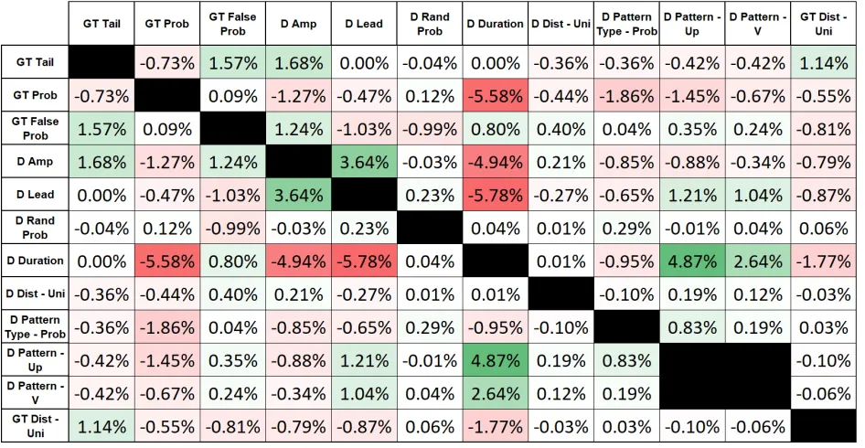
5.4.5. Landmark/Transformation Parameter Correlation 73
5.5. Landmarking System Testing 76
5.5.1. Test Data Generation 77
5.5.2. Effect of LSpliton Landmarking Performance 78 5.5.3. Effects of LN, LMaxon Landmarking Performance 79
5.5.4. Final Landmark Conclusions 82
6. Validation Experiment 83
6.1. Results 83
6.2. Validation Experiment Conclusions 87
7. Conclusions and Future Work 88
List of Tables
Table 1 - Sample Transformation Parameters 27
Table 2 - Sample Consecutive GTTest Instances Before and After Binning 29
Table 3 - GT Generation Parameters 32
Table 4 - D Generation Parameters 34
Table 5 - DPattern Values 35
Table 6 - DPatternType Values 36
Table 7 - Sample GT Parameter Values 38
Table 8 - Sample D Parameters 39
Table 9 - Screening Generation Parameters 41
Table 10 - Screening Transformation Parameters 41
Table 11- Raw Values Transformation Parameters 44
Table 12 - Test Parameter Values 48
Table 13 - Sample KNearestNeighbors Landmark Search 50
Table 14 - Sample Landmarking Knowledge Base 51
Table 15 - Sample Landmarking System Parameter Values 52
Table 16 - Landmark System Parameters 53
Table 17 - Screening Generation Parameters Results 57 Table 18 - 2-Factor Interaction of Generation Parameters 58
Table 19 - Predeterminable Features 61
Table 20 - GTDist Landmark Correlation Testing 63
Table 21 - DDist Landmark Correlation Testing 64
Table 22 - DAmp Landmark Correlation Testing 65
Table 23 - Final Landmarking Features 66
Table 24 - Limit Experiment Generation Parameters 67
Table 25 - Limit Experiment Transformation Parameters 68 Table 26 - Generation & Transformation Parameter Values Used for GTTL Limit Test 68 Table 27 - Generation & Transformation Parameter Values Used for GTProb Limit Test 69
Table 28 - Generation & Transformation Parameter Values Used for DAmp Limit Test 71
Table 29a & b - Landmark/Transformation P-Value (a) & Correlation Coefficients (b) 74
Table 30 - Landmarking Parameters Test Values 76
Table 31 - Landmark Testing Data Generation Parameters 77 Table 32 - Landmark Testing Transformation Parameters 78
Table 33 - Validation Testing F-Score Results 84
List of Figures
Figure 1 - Leading Indicator Time-Series Example ... 5
Figure 2 - Sample GT(a) and D(b) Data Streams ... 23
Figure 3 - Sample Spike Transformation before (a) and after (b) at s = 1 ... 25
Figure 4 - Lead Time Profiles... 26
Figure 5 - Spike Binning Transformation Example ... 27
Figure 6 - Maintaining Temporal Patterns: Transformation Method vs Aggregation ... 28
Figure 7 - Transformation System Overview ... 30
Figure 8 - DPattern Samples ... 35
Figure 9 - Sample Patterns Applied at DAmp = 1 (a) & DAmp = 4 (b) ... 35
Figure 10 - Sample Patterns Applied at DDur = 6 (a) & DDur = 10 (b) ... 36
Figure 11 - DPatternType Sample... 37
Figure 12 - Sample Event Distribution using GTProb = .05 & GTDist = Sine ... 38
Figure 13 - Sample Event Distribution using GTProb = .05 & GTDist = Uniform ... 38
Figure 14 - Generated D Raw Values ... 39
Figure 15 - Generated D with Pattern Applied ... 39
Figure 16 - Landmarking System Overview ... 51
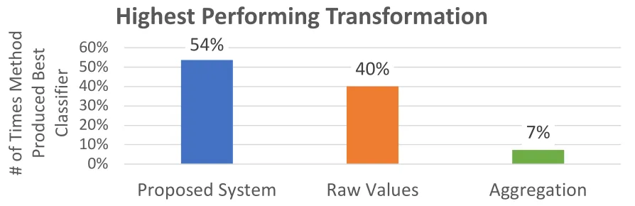
Figure 17 - Total Enumeration Test - Best Method ... 59
Figure 18 - F-Score Improvement from use of Transformation Method ... 60
Figure 19 - GTDist Coefficient of Variation Correlation ... 63
Figure 20 - DDist NRange Correlation ... 64
Figure 21 - DAmp Coefficient of Variation Correlation ... 65
Figure 22a & b - GTTail Limit Testing Results... 68
Figure 23a & b - GTProb Limit Testing Results... 69
Figure 24a & b - DAmp Limit Testing Results ... 71
Figure 25 - Sensitivity Limit Testing Results ... 73
Figure 26 - Effect of LSplit on F-Score Percentile ... 78
Figure 27 - Interaction Plot LN & LMax ... 80
Figure 28 - Prediction Timeline of Baseline vs Transformation Method at N=1... 85
1.
Introduction
Cyber-attacks have been the cause of massive loss of capital and damage to vital infrastructure in
both the private and public sectors over the last few years (Bronk & Tikk-Ringas, 2013;Lee,
Assante, & Conway, 2014). A large scale cyber-attack has the potential to cost the United States
government upwards of $121 billion dollars, more than the total damages of Hurricane Katrina
(Maynard & Ng, 2017). The rise of the “Internet of Things” has created wireless connections and
access between systems that have never before been remotely tethered. These vast networks can
result in very real risks to connected individuals (Roman, Zhou, & Lopez, 2013). In late-2016,
malicious software known as Mirai was able to take down multiple major sites such as Twitter and
PayPal by utilizing the computing power of millions of vulnerable devices connected through the
“Internet of Things” (Kolias et al., 2017). Although these connections are created for ease-of-use
and streamlining purposes, they drastically increase the risk of a devastating infiltration.
If businesses could see these types of attacks coming before they occurred, even without absolute
certainty of the time and place, they may drastically reduce their losses incurred. Forewarning
would allow for the focusing of security efforts and heightened defenses around a given network
during the expected window of the attack. While current approaches rely on network sensor
activity to detect cyber-attacks, the method is limited by the origin of the data being utilized. There
must already be unwanted access of or attempts on the network for these sensors to generate
The future of cyber-defense may lie in providing warning before an attempt on a system is even
made. Research has been conducted regarding the use of traditional forecasting methods such as
multi-correlation and ARIMA models in predicting the number of cyber-attacks that may occur in
a given time period (Pontes et al., 2011;Werner, Yang, & McConky, 2017). Forecasting models
utilize the rates at which cyber-attacks have transpired and attempt to decipher patterns or trends
that have predictive value moving forward. These models function by exploiting autocorrelations
in the data set, which may make generating predictions difficult for events which are very sparse
or follow no detectable trend or seasonality. Instead of trying to find a pattern within the timing of
the events themselves, more benefit may be found in examining external data, such as public
outrage or availability of malicious software tools, suspected of providing evidence or latent
indicators of attacks (Jordan, 2001;Ashford, 2012). Outside data sets which may contain predictive
value are known as leading indicators. The greatest difficulty lies in determining which data
streams function as leading indicators for cyber-attacks.
There has never been more data readily available to researchers than there is now. The types of
data available range from historical weather and environmental data to counts of traffic violations
issued in a geographical region (NOAA, 2017;MCoM, 2015). One major source of data which
appeared in 2006 and has grown rapidly ever since is Twitter. As of 2016, more than 500 million
tweets were created each day, with the number increasing every year (InternetLiveStats, 2017).
Numerous analytical techniques have been employed, both traditional and novel in their methods,
in attempts to make use of the wealth of available data. Tools to derive information such as public
sentiment and trending topics amongst populations from Twitter usage data have become popular
of Twitter data has been promising in some fields, such as social sciences and business, while
lacking in others, such as cyber security (Lerman & Ghosh, 2010;Chae, 2015). The promise of
valuable insight continues to drive research utilizing Twitter as well as other data sources for
predictive purposes in the realm of cyber-defense. The study in this thesis aims to approach the
predictive problem through the application of a novel method which may be used to extract
predictive patterns from many of the data sources mentioned.
Even though an individual or organization may have access to large amounts of data, how best to
derive useful information from a given data set is not always clear. Transforming a temporal data
stream containing millions of entries into a feature set which may be used to train a machine
learning algorithm involves numerous challenges. The difficulties faced include questions such as
how much historical data to incorporate, which classification algorithm to use, and how these
factors may influence the time required to train a desired algorithm. Simply training on all available
data is almost never the best approach and is often not possible due to constraints on run-time and
processing power. In the case of a time-series data set, many features of the data beyond just the
raw values may be used, such as trends and statistical characteristics (Meina et al., 2015). The
“Curse of Dimensionality” often comes into play, with each additional feature extracted from a
data set creating a more complex training process while potentially adding little to no value
(Friedman, 1997). Without active reduction, a feature set can rapidly become too complex to train
a classifier within a reasonable amount of time.
The practice of reducing the data used for training and extracting useful features may be referred
is too large or complex to use into a manageable form. Feature engineering may involve
aggregating multiple values into one, removing unneeded features that provide little or no value to
the task at hand, or finding value in the interactions of features. Unfortunately, the best approach
to engineering the features of a data set to make them more useful is not always clear.
While many approaches to improve the predictive power of a given data set exist, no best fit
method will apply to more than a specific assortment of similar data sets. Single-featured,
time-series data sets may be particularly difficult to extract information from if they contain no trend or
seasonality. A given time-series data set may contain predictive information over any range of
time or type of pattern. The challenge is now determining an efficient and automated method to
extract maximum predictive value from a range of single-feature time-series data streams. Once a
method is developed, available time-series streams which meet the necessary input format may be
utilized in a more effective form to attempt to forecast oncoming cyber-attacks. Even without high
precision, any method to provide forewarning of cyber-attacks could be very useful. In the realm
of predicting a major attack, a false positive warning is far less harmful to a target than failing to
2.
Problem Statement
All the relevant data in the world is of no use when solving a problem if the data cannot be
practically applied. Large data sets regularly require extensive dimensionality reduction to be used
in the training of machine learning classifiers. Although the problem of extracting value exists for
all data types, time-series data can be particularly challenging to use efficiently. Time-series data,
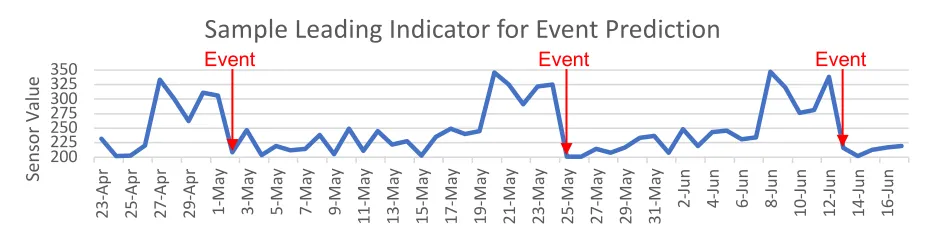
such as the sample shown in Figure 1, is defined as a sequence of observations recorded at distinct
time intervals and stored in chronological order, usually recorded over successive time intervals
with consistent spacing. A time-series data stream can represent anything from barometric pressure
[image:14.612.75.539.338.455.2]to occupants of a building at various points in time.
Figure 1 - Leading Indicator Time-Series Example
An acquired data stream may be used to generate predictions against a provided Ground Truth
(GT). The GT is a data series containing the time-stamps of occurrences of an event type to be
predicted. Training a classifier on the GT series requires converting the provided time-series data
stream into a useable feature set. Training on the entire time-series is often infeasible and almost
never the best approach, as each data point would be handled as a separate feature by the classifier
and dimensionality could become a problem. The challenge becomes developing an algorithm to
reduce time-series data in order to condense the resulting feature set while extracting significant
predictive value and retaining the temporal nature of any trends or patterns. 200 225 250 275 300 325 350 23-Ap r 25-Ap r 27-Ap r 29-Ap r 1-M ay 3-M ay 5-M ay 7-M ay 9-M ay 11-M ay 13-M ay 15-M ay 17-M ay 19-M ay 21-M ay 23-M ay 25-M ay 27-M ay 29-M ay 31-M ay 2-Ju n 4-Ju n 6-Ju n 8-Ju n 10-Ju n 12-Ju n 14-Ju n 16-Ju n Se nso r V al ue
Sample Leading Indicator for Event Prediction
The purpose of the research moving forward is to determine an efficient, automated, and effective
method to extract useful feature sets from time-series data streams for use in predicting if an event
will occur on a given day or not. A series of transformations will be performed on single-feature
time-series data streams to determine how each transformation must be applied for best
performance. The transformations are meant to clarify or retain patterns that exist in the data while
reducing the size of the feature set being used to train a classifier.
The transformation parameters to be determined by the process include lead time of predictions
(lead time), length of data used for feature set creation (tail length), the length of aggregation
periods used (bin size), and sensitivity to abnormally high values, referred to as spikes, in the data
(sensitivity). The resulting feature set extracted from the transformed data will be used to train
classifiers for event prediction. The process has been designed to both reduce the feature set for
the purpose of faster classifier training as well as extract maximum predictive value from any
pattern that exists within the provided data set.
Testing the transformation method will involve measuring the performance of classifiers trained
on the transformed feature sets versus classifiers trained on a baseline feature transformation. The
baseline features will be a set containing the untransformed time-series values. The performance
of baseline features will be compared to the performance of the transformed feature sets to
determine if performance was improved. The significance of the performance differences will
A system to utilize prior knowledge to predetermine a best fit transformation set and classifier type
will also be developed and tested. Testing of the prior knowledge selection system, further referred
to as the landmarking system, will be conducted using generated data stream and event set pairs.
The generation of artificial testing sets will allow for a set of controllable generation parameters
determining event frequency and distribution, as well as the shape of predictive patterns in the data
stream. The transformation and classifier combination selected by the landmarking system will
then be compared to the performance of all transformation sets recorded to determine the
significance of the tradeoff in classifier performance. The effect of varying the number of top
performing similar transformations selected by the landmarking system will be examined as well.
The testing process will determine the landmarking system’s capability to accelerate
transformation set selection without significant performance loss. If the landmarking system is
able to select a transformation set that creates a classifier close enough to the best observed
transformation while also saving a significant amount of run time versus total enumeration, the
system will be considered successful. The other significant performance measure is whether the
best observed classifier produces a statistically significant performance improvement over the
baseline feature set. The results of the experiment will determine whether the transformation
process paired with the landmarking system yield a significant improvement or not.
The purpose of the transformation method is to convert single-feature time-series data into a form
which clarifies predictive patterns and improves classifier performance. The method may be used
to find the predictive power of a provided time-series data stream. The ability to do so would be
complete data reduction, feature extraction, and classifier selection in an accelerated way using the
landmarking system would allow for testing to be conducted on more data streams in less time
than could be achieved through total enumeration. The likelihood of producing a useful feature set
3.
Literature Review
Review of literature pertaining to cyber-attacks, feature engineering and classification methods
was conducted to establish a “best-practice” wherever possible in developing an automated feature
engineering system. Understanding what methods have been conducted in creating better
cyber-attack prediction methods ensures that the proposed research does not retrace any previously tested
models. While the system focuses on the intelligent feature engineering of time-series data streams,
methods used previously on both time-series and non-time-series data can reveal techniques that
may be tested, and if successful, included in the final system. The final piece of the proposed
method is the classification method being employed to create a prediction from the transformed
data stream. While finding the best values of the classifier parameters themselves is not the primary
focus of the proposed research, being a data transformation experiment, confirming that the
classifiers tested are appropriate for the task at hand, and will yield useful testing results, is
important to the experiment as a whole.
The literature review begins with an evaluation of current methods being applied to the forecasting
of attacks. Models and methods which are shown to be effective in the realm of
cyber-security prediction are used to help develop the approach of the proposed system. In addition to
determining research methods that have been shown to be effective, determining where they have
fallen short assists in guiding the newly developed method towards a novel objective. The next
section of the literature review examines current feature engineering techniques to determine what
methods yield performance improvement. The following section provides background on the
application and performance of the classifiers that are to be included in the automated feature
classifier, which will be adopted for use in the proposed system. The section also discusses the use
of meta-features to improve selection of the transformations and classifiers used in the proposed
research.
3.1.
Event Prediction Using Forecasting and Machine Learning
Forecasting techniques are commonly used to generate predictions using a time-series data set.
One study reviewed tested the application of an ARIMA model to the field of cyber defense in
event prediction(Werner et al., 2017). In the model, time-series data containing information
regarding the time and type of cyber-attacks is used to train a forecasting method meant to predict
the number of cyber-attacks on a given day.
When tested on historical attack data, the ARIMA model followed spikes in occurrence data, albeit
with some lag behind the initial spike, indicating that using ARIMA forecasting leads to better
performance than simply following the mean. Prediction error for less frequently occurring events
such as denial of service or malicious URL was twice that of attacks on internet facing servers, in
part due to forecasting methods performing better when the data set being examined contains a
fewer number of zeros. One of the limitations of ARIMA forecasting is that increasing sparsity in
data has a negative performance impact. The data patterns contained in the test data used in the
proposed thesis may also be sporadic and difficult to identify on a large scale, which can lead to
reduced performance using traditional forecasting methods.
Experimentation has also been conducted using a Bayesian Network to attempt to predict
signals into the training of a Bayes Net. Once all the signals are formatted, an individual Bayes
Net is trained for each of the five types of attacks being investigated.
Through 5-fold cross validation testing Bayes Net was found to perform well on more frequent
attack types while failing to predict any of the sparse DDoS events. The results reflect an issue of
the Bayes Net valuing precision in negative event prediction over positive event prediction when
trained on sparse data (less than 9% occurrence rate).
Research conducted using a Support Vector Machine and the traffic of malicious IPs showed the
method effective at predicting cyber-attack incidences up to 3 months prior to their occurrence
(Liu et al., 2015). A feature set was generated to capture the behavior of malicious IP addresses in
a way which reveals anomalies in their behavior as individuals as well as a group. Testing was
performed using subsets of these features to determine which features yielded the greatest
performance gain. The study validated the use of a separate set of leading indicators to predict the
timing of a major attack on the Univ. of Maryland. All 3 classifiers were capable of indicating a
high risk of an oncoming attack, however, an interesting result was that the highest performing
classifier was that trained only on Nov-Dec-Jan data rather than Nov-Dec-Jan-Feb data. The results
indicate that the classifier may achieve highest performance with a certain amount of lead time >1
day.
Another research team developed a method to create a general cyber-attack forecast built on
Japanese tweet counts and the activity of Twitter accounts of 90 know hacktivist groups
the tweets of hacktivist groups. An artificial neural network (ANN) was trained and tested using
these factors on 34 unique cyber-attack events.
Results of the experiment show that the activity of accounts known to be linked to cyber-attack
display a pattern of higher than average activity during the month prior to an attack occurring for
all events tested. The experiment also stated that a limitation of examining the hacktivist data was
the sparsity of activity, where the data examined in the proposed thesis is more densely populated,
providing the capability to examine the time frame preceding each cyber-attack with more
granularity.
Major issues, such as predicting infrequent events, faced with each of these methods are addressed
through the transformation method applied in the proposed thesis. Predicting infrequent events is
difficult using the aforementioned forecasting or Bayes Net approaches because of their innate
tendency to predict all negative for a sufficiently sparse event type, resulting in high precision, but
providing little real value. By using the new method being investigated to utilize recognizable data
patterns as opposed to single aggregated values, the classifier will be better able to predict sparse
events. Creating a method meant to accurately predict when sparse events occur could complement
a traditional method by being used on attacks below a set occurrence rate. Liu et al., (2015) shows
SVM’s validity for predicting cyber-attack and for utilizing large feature sets. Liu et al. also
suggest that prediction accuracy may be maximized through testing on lead times > 1 day, which
will be incorporated into the developed transformation system. Munkhdorj & Yuji, (2017) shows
that analysis of Hacktivist groups provided some predictive value. The data to be used for the
information known to coincide with malicious activity are contained. The combination of utilizing
a more correlated, closely populated data set as well as the testing of multiple classification
methods is expected to clarify the predictive value of the detected activity increase prior to attack
occurrences.
3.2.
Feature Reduction and Extraction
The data sets examined through the proposed research are numerical counts in the form of
time-series data streams. The temporal data provides a basis from which forecasts or predictions may
be generated, often used to estimate future events or behaviors (Antunes & Oliveira, 2001). Most
time-series data streams contain a vast number of values, many of which may provide little
predictive values in their initial form. For example, a data set containing the readings of 10 sensors
within a system each providing a reading every 2ms would generate 5000 unique values/ second.
Perhaps the user is interested in predicting an event which is influenced by the difference in 2 pairs
of these sensors as opposed to the raw values of all 10. In addition, the event being predicted may
be preceded by spikes every 30 seconds. An improved data set may contain only the differences
between the 2 sensor pairs and an aggregated value for each second. Through the proposed
transformation, the data set would be reduced from 5000 features and 10 unique values/second to
2 features and 1 value/second. Reducing data sets through similar feature reduction techniques,
such as aggregation, removal, and similar transformations, is a key focus of the proposed
transformation method.
The goal of feature engineering techniques is to remove features which provide little or no
time of classifiers, as well as reducing “noise” which negatively affects the accuracy of predictions
generated. The aggregation of numerical features may be achieved through a variety of reduction
techniques such as summation, averaging, or many other methods.
Another study examined utilized multiple data transformation techniques in order to create useful
features out of 2 large data sets (Yu et al., 2010). The method used involved assessing performance
metrics of a set of students in order to predict their future performance. After creating categorical
features to identify question type, student id, and other identifying characteristics, the first data set
had approximately 1,000,000 unique features and the second data set had approximately 200,000
unique features. Training classifiers on these data sets remained infeasible due to training
time/processing power restrictions.
To reduce the number of features in the student data, past performance metrics on identical
question types were averaged to create a single past performance measure for each question type.
In addition to averaging matching features, single features were generated for each student, each
identical problem type, etc. which measured the percentage of attempts which were correct the
first time. Another transformation technique employed was creating a set of 4 binary features
indicating student familiarity with a given question type, indicating if a student had encountered a
given problem type within a prior window of time. The final data sets used in the research project
had been reduced from more than 100,000 features to only 17.
Performance was measured first using the untransformed data set, followed by the 17-feature data.
performance was achieved using both of the condensed data sets compared to using the
untransformed data. The results display that a massive reduction in features, 99.9983% and
99.9915% respectively, was achieved without sacrificing significant performance. These types of
transformations extract the useable information from patterns within a data set and are similar to
those being employed in the transformation system being developed. The performance
improvement achieved shows the promise of being able to extract and simplify the meaningful
value of a large data set down to a small set of features through feature engineering.
The Heritage Health Prize (HHP) competition focused on predicting the likelihood of patients to
be admitted to a hospital based on historical data("Heritage Health Prize," 2012). The first-place
team used two distinct methods of feature reduction in order to create multiple testing data sets
(Brierley, Vogel, & Axelrod, 2011). The first method employed by the researchers was yearly
aggregation, resulting in (# of years * # of unique patients) instances to be trained on. The second
method tested was aggregating all claims by patient. The combined results yielded a .0035
improvement in root-mean-square error over what any one model could achieve on the original
data sets, a significant improvement with the difference between the 1st and 5th place teams being
<.002. Using the described method of aggregating multiple data sets over varied aggregation
periods could yield both higher performance than using a single test set in the proposed
transformation system.
In the AAIA’15 Data Mining Competition competitors were tasked with classifying the
research team used histograms of occurrence frequency within the 42 unique time-series data
streams per firefighter to train a Support Vector Machine (SVM) (Zdravevski et al., 2015).
Testing results showed that when the team aggregated the provided data streams into small
windows of time, with the total number of aggregation periods referred to as B, the use of more,
and therefore smaller, aggregation windows frequently resulted in overfitting of the SVM. The top
14 performing classification methods used only B = 30 or B = 50 while B = 100 resulted in reduced
predictive performance.
The results of the study suggest that training on only the most valuable portion of the training data
rather than the full data stream improves classifier performance while reducing complexity and
training time. The method of generating training histograms employed in the experiment sacrifices
the temporal component of the data set, which the proposed thesis system seeks to retain through
utilizing a similar binning process aggregated by time as well as value.
3.3.
Classification Methods
An algorithm, or machine learning model, may be trained to classify an outcome based on a set of
values provided. The value set provided are related to a set of features common to the data set
upon which a given classifier was trained. Classification algorithms allow predictions to be made
regarding the likelihood of an event occurring through examining one or more related data sets.
Classification methods use a variety of algorithms to determine how best to classify a given
prediction differs, which may result in different classifier types producing different results when
provided the same data set for training and testing.
The classifiers used in the proposed thesis are binary classifiers which predict 0 or 1 when given a
set of features. An algorithm for classifying new instances is generated based on the correlation
between values of the features of examined instances and their respective categories. The use of
labeled examples for training is known as supervised learning, as opposed to unsupervised learning
in which the algorithm must generate classes within the data (Brownlee, 2016).
The “No Free Lunch” theorem stated that one cannot determine a best fit classification method
based on prior knowledge alone, the classifier must be tested against a ground truth. Different
classification algorithms may be more effective in handling factors adverse to effective machine
learning such as sparse data sets or vast feature quantities. Because of this, multiple distinct
classification methods will be incorporated into the system to allow for the widest range of
classifiers tested per dataset. In order to conduct the study on a large number of classifiers in a
practical way, the WEKA machine learning library will be utilized (Frank et al., 2009). The WEKA
classifiers to be tested in the experiment are an Unpruned Classification Tree, a K-Nearest
Neighbors algorithm, a Bayes Net and an SVM classifier.
The Classification Tree and KNN algorithms will be included as both have shown to provide
differing results with reasonably consistent performance in a previously discussed meta-learning
experiment (Reif, Shafait, & Dengel, 2011). Because these two classifiers utilize fundamentally
Decision Tree, they will function well early in the research for comparison. Random Forest, an
extension of the Decision Tree algorithm will not be used for the research case as the training
demand would be much higher than a Decision Tree. Any additional predictive performance
Random Forest would provide is unneeded as measuring performance changes across different
data transformations is more important to the experiment than overall precision of the classifier.
The Bayes Net classification method was selected due to robustness when handling many features
which have little predictive value as well as use in similar research examined (Okutan et al., 2017).
The SVM classifier has been shown to be effective in previous research regarding data
transformation testing so will be included in the proposed thesis (Liu et al., 2015;Meina et al.,
2015).
3.4.
Meta-Features for Classifier Selection
Determining a best fit classification method has been a problem since the origin of machine
learning. According to the “No Free Lunch” theorem, first proposed by David Wolpert, one cannot
determine what supervised classification method will yield the best results based on prior results
alone (Wolpert, 1996). One method proposed for solving the problem of finding a best performing
classification method is through landmarking (Bernhard, Hilan, & Christophe, 2000).
Landmarking was developed through a study in which the landmarking system was used to predict
a best fit classifier through the performance results of a small set of experiments, or “landmarks”.
Landmarks are algorithms which have performed successfully on a specific data set, or better yet
Meta-features are features which exist as a quality of the data set as a whole. Research into a field
referred to as “meta-learning” aims to study the effect of “meta-features” on the performance run
times of classifiers (Doan & Kalita, 2016). Simple meta-features refer to features pertaining to a
data set such as number of features, number of classes, number of instances, etc. which do not
require extensive calculation to be derived from the data set. Applying transformation methods in
a novel way to time-series data as well as utilizing meta-features to improve performance is the
primary objective of the proposed research.
A study was also conducted with the intent of examining the effects of simple meta-features on
the run time of different classification methods (Reif et al., 2011). The results gathered through
the testing of 5 classifiers (KNN, SVM, MLP, Ripper, Decision Tree) on a traditional grid search
problem suggest that there is significant correlation between the values of a set of “simple
meta-features” and the run-time of a given classifier. The normalized absolute error of the predicted
runtimes of each of these classifiers using only simple meta-features was ~.6, resulting in 40%
lower error than when not considering these features. In addition to demonstrating that reducing
the factor set assists with altering run-time, the results show that examining meta-features with
relation to transformed data sets in the proposed system may allow for identification of data sets
with beyond feasible run-times before they are tested.
The meta-features of the data sets which result in their similarities are then identified. By grouping
a new data set with which there is no prior testing with other data sets based on its meta-features,
the classifier which has the best performance on the similar data sets may provide a good starting
study and discovered promise for application of the system in improving classifier selection. A
similar method can be employed in attempting to determine which classifier and transformation
values may work best on a given data stream, using features such as the number of events in the
event set, variance of the values within the data set, length of historical data available for training,
4.
Methodology
The methodology first introduces the proposed transformation developed and tested for the study.
Once all steps of the transformation process have been examined and their application as a single
process is presented, the experiment for testing the transformation process is introduced. The
process of generating test data sets to measure the performance of the transformation process is
explained in depth followed by the procedures used to narrow down these data sets and
experimental parameters for more efficient testing. The proposed method of measuring the
performance of the transformation process and validation testing using real data is then proposed.
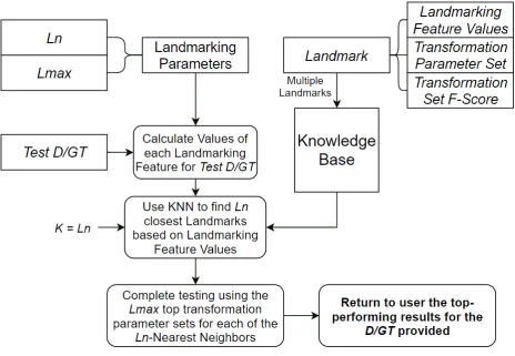
Section 4.3 of the methodology introduces the landmarking system and explains how the
landmarking system is intended to improve the efficiency of the proposed transformation method.
The functionality of the landmarking system is then explained as a step-by-step process to detail
the purpose of the system. Finally, an approach for measuring how effectively the landmarking
system performs and an experiment designed to measure the system’s performance is laid out. The
last section covers exactly what performance measures were collected and how they were used to
gauge the usefulness of the landmarking system.
4.1.
Transformation Method
The method used in the proposed research requires a specific format of data to perform certain
transformations. The restrictions on the format of the data, requiring a time-series numerical data
stream and set of event time stamps, are key to the operation of the process as a whole. Some
approaches are used to modify the provided data streams to enhance the performance of the
The proposed method applies all transformations put forth by the study. The transformations
include spike conversion, which involves transforming the data set from a data stream with a
continuous range of numerical values to a set of binary values. Additional transformations include
reducing the number of data points considered for training, known as tail length, as well as testing
differing spans of time intervals between the data to be trained on and the event to be predicted,
known as lead times. The final transformation used involves aggregating these data points into
bins of a predefined width.
4.1.1.
Transformation Method Input
Input Terminology
D Continuous single-feature time-series data stream to be used as a leading indicator
GT Series of time-stamps of events to be predicted by the trained classifier
The instances within the provided time-series data stream each contain a timestamp and
corresponding value. These sets may contain 0 values, however the “Time” column must be
uniform with no missing values. Having no missing values allows the transformation method to
better identify temporal patterns without inconsistent spacing of time-intervals. Formatting of data
streams and backfilling of missing values was not considered part of the core program tested and
was handled through external scripts. Each instance Di consists of a time Di,t and level Di,l.
A data set containing the timings of events to be predicted must be provided in order to train the
classifiers as well as generate performance metrics. After removing any duplicates, the stream of
individual instances GTi. Partial examples of appropriate supplied D and GT data sets, prior to
removal of GT duplicates, are shown in Figure 2.
GT is then subdivided into a training set, GTTrain, and a testing set, GTTest, such that:
𝐺𝑇#$%&'∪ 𝐺𝑇#)*+ ≤ 𝐺𝑇 (1)
after removal of duplicate event dates. In order to train the classifiers using GTTrainboth positive,
𝐺𝑇-.*&+&/) #$%&', and negative, 𝐺𝑇0)1%+&/) #$%&', event instances must exist within the data set such
that:
𝐺𝑇-.*&+&/) #$%&' + 𝐺𝑇0)1%+&/) #$%&' = 𝐺𝑇#$%&' (2)
Having close to a 1:1 ratio between positive and negative occurrences in GTTrain is preferred in
order to avoid generating a biased classifier (Kubat & Matwin, 1997). Therefore, simply using all
dates not contained in 𝐺𝑇-.*&+&/) #$%&'as negative occurrences, although valid, was not the chosen
method for the experiment. The approach taken for the purpose of the research is to calculate a
time centrally positioned between each 𝐺𝑇-.*&+&/) #$%&',&,𝐺𝑇-.*&+&/) #$%&',&67 timestamp pair where:
𝐺𝑇-.*&+&/) #$%&',& = 𝑡𝑖𝑚𝑒 𝑜𝑓 𝑖+>𝑒𝑣𝑒𝑛𝑡 𝑜𝑐𝑐𝑢𝑟𝑎𝑛𝑐𝑒 𝑖𝑛 𝑡𝑟𝑎𝑖𝑛𝑖𝑛𝑔 𝑠𝑒𝑡 (3)
𝐺𝑇0)1%+&/) #$%&',& = G𝐺𝑇-.*&+&/) #$%&',&+ 𝐺𝑇-.*&+&/) #$%&',&67
2
∀ 𝑖 𝑖𝑛 𝐺𝑇-.*&+&/) #$%&' 𝑤ℎ𝑒𝑟𝑒 𝑖 ≠ 𝑖 + 1
(4)
DDoS Attack Dates Daily Twitter Mentions
Figure 2 - Sample GT(a) and D(b) Data Streams
These times are used as the 𝐺𝑇0)1%+&/) #$%&' for training purposes so as to provide maximum
disparity between the spike profiles of positive and negative occurrences. The process of creating
an equal number of positive and negative GTTrain events is referred to as leveling the training set.
In the case of a 𝐺𝑇-.*&+&/) #$%&',&,𝐺𝑇-.*&+&/) #$%&',&67 pair occurring at sequential times, no negative
event is generated and the 𝐺𝑇-.*&+&/) #$%&',&67 event is removed.
The process for creating the negative events of GTTest involves simply labeling every time instance
not contained within the provided event set as a negative occurrence. The creation of these negative
occurrences is done under the assumption that the provided GT is complete for the associated span
of time contained. GTTest cannot have empty or irregular time-intervals in order to allow the
classifier to test on each time instance in sequence.
4.1.2.
Spike Transformation
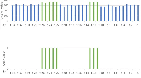
The first transformation applied to each data stream is a conversion from the individual raw values,
referred to as Di,l, to individual “spikes”, referred to as Pi. The most basic application of the spike
transformation utilizes the formula:
𝑃& = O1 𝑖𝑓 𝐷&,Q ≥ 𝑠𝜎 + 𝜇
0 𝑜𝑡ℎ𝑒𝑟𝑤𝑖𝑠𝑒, (5)
where s is sensitivity or number of standard deviations and σ is the standard deviation of the values
of Dland µ is the mean of Dlin the training set. The transformation to spikes is meant to clarify
patterns of abnormally high values in the data set and reduce the raw values to a set of binary
values, resulting in a simplified training process. An example of an application of the spike
Figure 3 - Sample Spike Transformation before (a) and after (b) at s = 1
The spike transformation is also used to normalize values across multiple data sets, allowing for
easier inclusion of additional data streams and potential cross-set transformations such as
combining spikes with matching time-stamps. The transformation may be modified through
varying the number of standard deviations (σ), referred to as sensitivity s, above the mean
necessary for a value to be transformed into a “spike”, as well as testing numerical transformations
on values based on how many standard deviations over the mean they are.
4.1.3.
Determining Tail Length and Lead Time
Further transformations to be tested include adjusting the number of data points included in each
training set, referred to as Tail Length (TL) and testing the method over a variety of lead times (N),
the number of data points prior to the event being predicted at which the training set concludes.
0 100 200 300 400
t-34 t-32 t-30 t-28 t-26 t-24 t-22 t-20 t-18 t-16 t-14 t-12 t-10 t-8 t-6 t-4 t-2 t0
Or ig in al V al ue 0 1
t-34 t-32 t-30 t-28 t-26 t-24 t-22 t-20 t-18 t-16 t-14 t-12 t-10 t-8 t-6 t-4 t-2 t0
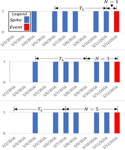
The lead time parameter is illustrated in Figure 4 as N and allows a classifier to train on patterns
occurring greater than 1-time interval prior to an event.
TL is varied as a parameter of the transformation method to determine the minimum amount of
data to be included while improving predictive performance. In addition to the specified tail length
TL, the value of the lead time N for a given test affects which data points are analyzed leading up
to an event time. For N = 1, the spike profile used to train consists of the data points immediately
preceding the event time. If N > 1, the spike profile must be shifted to account for the gap between
the event to be predicted and the time at which a prediction is generated.
4.1.4.
Creating Binned Spike Profiles
Once the data stream has been subsetted into TLlength training sets with lead time N,the spikes
[image:35.612.74.286.130.385.2]are aggregated into a set number of bins (Bi), where i = bin location in array. The width of each
bin, A, is another parameter of the transformation method which was varied in testing. All Pi within
the bin are summed following the formula:
𝐵& = W 𝑃& X&
&Y76X(&[7)
(6)
to generate the value of Bi, which is then appended to the training set. An example transformation
using the parameters in Table 1 is shown in Figure 5.
Table 1 - Sample Transformation Parameters
Parameter Value
TL 8
A 4
Figure 5 - Spike Binning Transformation Example
Because the generation of Bi’srelies on the aggregated values at each time stamp, only factors of
TL are used as values of A in the testing process.The process of binning Pi’s into Bi’s to construct
a spike profile B with length #]
The binning process is meant to both reduce the number of features required to train a classification
engine, as well as expose underlying trends or patterns in the training data. The bins are expected
to capture irregular patterns in a form more useful for classification than raw values would. Within
a given pattern, activity at a particular point in time may matter less than activity over a span of
time, which a bin captures.
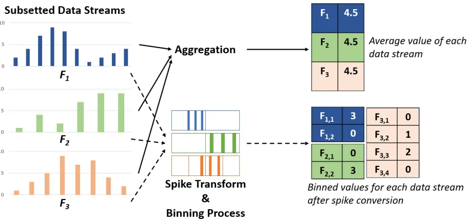
The binning process also holds a distinct advantage over total aggregation of a training set through
maintaining temporal patterns. An example of how a pattern may be lost through aggregation is
[image:37.612.82.537.329.544.2]shown in Figure 6.
Figure 6 - Maintaining Temporal Patterns: Transformation Method vs Aggregation
As shown through the conversion of the three subsetted data streams to feature sets, total
aggregation views all data streams identically while binning maintains the temporal patterns while
Table 2 shows an example of two consecutive instances that could be contained in GTTest, along
with the values of each feature of these instances both before and after their spike values have been
binned using A = 2.
Table 2 - Sample Consecutive GTTest Instances Before and After Binning
F1 F2 F3 F4 F5 F6 F7 F8 Event
0 1 0 0 1 1 1 0 1
1 0 0 1 1 1 0 0 0
F1 F2 F3 F4 Event
1 0 2 1 1
1 1 2 0 0
4.1.5.
Transformation Process Overview
A process to identify the best set of transformation parameters is shown in Figure 7 and functions
through being provided with both a time-series data set D as well as a set of event times known as
the ground truth GT. The GT is then leveled resulting in an equal number of positive and negative
events to provide an unbiased training set, after which transformations are applied to Dl, the values
of D, based on the timing of both the positive and negative events in GT. The transformations
involve first converting the time-series values into a binary set using the spike transformation. The
tail length TL and lead time LT are then used to subset the data and adjust the number of data points
used for each event prediction. The values are then aggregated into bins Bi containing a predefined
number of data points A as a reduction technique to create both a training and testing set to be used
Figure 7 - Transformation System Overview
After all transformations have been performed, the transformed training sets are used to train a
classifier using the GTTrain event set. After training, the classifier is then used to predict events. In
the case of the testing process, the events being predicted are those contained in GTTest. Each
time-interval of GTTest is used to create a unique training set based on the defined transformation
parameters. The training set is then used by the trained classifier to create a prediction of whether
the time-interval in question contains an event. Performance is then measured based on how well
4.2.
Transformation Method Experimentation
The following sections cover in detail how the data used to test the proposed transformation
method and landmarking system was generated. Performance metrics were gathered through the
process’s predictive accuracy when trained on all points of each generated GTTest. Methods for
reducing the number of generation parameters through a screening experiment and levels at which
these parameters must be tested through a limit experiment are discussed. The approach to testing
the transformation process used in the study is explained, as well as how the transformation process
was tested on a real data stream for validation of the proposed method. The effectiveness of the
proposed process when tested on real data was measured by performance improvement compared
to when no spike transformation is applied and A = 1, representing the raw values.
4.2.1.
Data Set Generation
In order to test the developed transformation method, testing data sets were generated using a
known set of parameters. These parameters will allow for analysis of the effects of particular
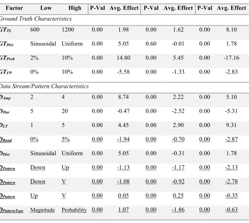
variables on the method’s ability to detect and utilize patterns. The effect of each of these
generation parameters were analyzed through a screening experiment to allow for the elimination
of any parameters with little effect or no further value to the research being conducted. Following
the screening experiment, a limit experiment was conducted with the purpose of establishing
effective upper and lower values at which to test the generation parameters.
4.2.1.1.
Data Set Generation Procedure
A controlled experiment was conducted to determine how well the transformation process
characteristics. The experiment first involved generating GT event sets with different distributions
as to when and how often events occur. By testing on a variety of GTs determining limitations or
highest performing event distributions in terms of prediction accuracy of the generated classifiers
is possible. For each of the GTs, multiple D data sets were generated containing different predictive
patterns and noise levels in Dl. By testing on multiple Ds for each GT, features of Dl and the
contained patterns may be altered and their effects on predictive performance measured.
Artificial GTs were generated to allow for performance testing of the developed method on a
variety of event distributions and frequencies. Each artificial GT was generated by applying a
probability distribution over a specified span of time to determine the likelihood of each time stamp
containing an event. The parameters affecting the GT set are shown in Table 3.
Table 3 - GT Generation Parameters
Parameter Description Test Values
GTTL Time intervals covered by GT 50, 100, 200, 500
GTDist Probability distribution of an event occurring on a given
day
Uniform, Sine
GTProb Average likelihood of an event across the entire GT .05, .10, .20
GTFP Likelihood of any generated event being a “false
positive”
.10, .25, .50
The number of points in time considered for the GT is determined by the value of GTTL. The
frequency of GT events and their distribution along the length of the GT are determined by GTProb
and GTDist. GTProb is a probability distribution spanning the length of the entire GT. The probability
GTProb determines the mean probability of GTDist, providing a way of estimating the number of
events to be generated based on the equation:
𝑇𝑜𝑡𝑎𝑙 𝐺𝑇 𝐸𝑣𝑒𝑛𝑡𝑠 ≈ 𝐺𝑇#a × 𝐺𝑇-$.c (7)
In addition to the generated GT events, a certain number of negative events are created to generate
uncertainty amongst the GT set. Each negative event is included in the GT when the predictive
pattern is applied to D, but then removed prior to testing. Following the given procedure, the
predictive pattern appears in D, but the corresponding event does not exist. GTFP is the probability
that any generated event is treated as a negative event. Using these artificial GTs allows for a set
of controllable parameters to be varied in order to determine the effect of various factors on
predictive performance.
From each of these artificial GTs multiple test data sets D are generated. The generated Dlcontains
a specified number of data points which follow either a Uniform or Normal distribution. Because
the process functions through detecting anomalous values based on standard deviation, the specific
mean and standard deviation of each data set does not affect performance. Each artificial D
The parameters contained in Table 4 control the generation of the base data points contained in Dl
as well as many of the characteristics of the pattern applied.
Table 4 - D Generation Parameters
Param Description Sample Values
DPattern Predictive pattern used Upward, Downward, V
DPatternType How the predictive pattern is applied Magnitude, Probability
DAmp Size of generated pattern spikes in
standard deviations
.5, 1, 2
DDur Number of data points over which
predictive pattern is applied
5,10,25
DLT Number of data points prior to event
at which predictive pattern ends
1,3,5
DRand Chance of each spike in a given
pattern occurring in D
.25, .5, .75, 1
DDist Likelihood distribution used to
generate values between [0,100]
Uniform, Normal
DDist determines the random distribution applied to the base values generated for Dl before any
predictive pattern is applied. The distribution determines how many “spikes” naturally occur
within the data set, with a uniform distribution producing ~16% spikes and normal distribution
producing ~29% spikes at s = 1. DPattern is the predictive pattern applied to each event.
Table 5 describes the distributions defined by DPattern. The patterns areused to create spikes during
generation of each artificial D using the defined parameters. Each of these distributions produce a
probability curve spanning DDur. The probability distributions of each DPattern allow for
Table 5 - DPattern Values
DPattern Shape Probability of Spike at 𝑫𝑮𝑻𝑻𝒓𝒂𝒊𝒏𝒊6𝒋,𝒕 while 0 ≤j ≤ DDur
Upward Linear Slope 𝑃 m𝐷n#opqrsr6t,+u = 1 𝐷vw$∗ 𝑗 Downward Linear Slope 𝑃 m𝐷n#opqrsr6t,+u = 1 − 1
𝐷vw$∗ 𝑗
V 2xLinear Slope 𝑃 m𝐷n#opqrsr6t,+u = ⎩ ⎨
⎧2 −𝐷2
vw$∗ 𝑗 𝑤ℎ𝑒𝑟𝑒 𝑗 = [1: 𝐷vw$
2 ] 2
𝐷vw$∗ 𝑗 𝑤ℎ𝑒𝑟𝑒 𝑗 = ( 𝐷vw$
2 : 𝐷vw$]
Figure 8 shows each of the values of DPattern listed in Table 5 as they would appear applied to a
sample data set D.
Figure 8 - DPattern Samples
DAmp controls a multiplier determining the amplitude of the predictive pattern being used. The
value of DAmpsets the number of standard deviations of each spike leading up to an event. A
sample of what two patterns applied using different values of DAmp may look like in the same D
are shown in Figure 9.
Figure 9 - Sample Patterns Applied at DAmp = 1 (a) & DAmp = 4 (b)
DDur determines pattern duration by specifying the number of data points over which the predictive
pattern is applied prior to each event. Examples of two different values of DDur are shown in Figure
10.
Figure 10 - Sample Patterns Applied at DDur = 6 (a) & DDur = 10 (b)
DLT defines the lead time of each pattern, or the number of data points prior to each event that the
predictive pattern ends. DLT should always correlate with a best lead time for event prediction.
DRand creates variability within the predictive patterns. DRand is a likelihood that any given point in
a pattern occurrence is not generated. If not generated, the value is left as the original generated
value of the given point.
Table 6 defines the methods through which the distribution defined by DPattern is used to apply a
pattern to the given data stream, referred to as DPatternType.
Table 6 - DPatternType Values
DPatternType Description
Magnitude P(Di) used as multiplier for amplitude of spike, defined by DAmp, occurring at point i
Probability P(Di) used as probability of spike occurring at point i
The first DPatternType method is magnitude, in which case the pattern value determined by DPattern at
a given point defines the amplitude of the spike occurring at the specified point. In the case of a
magnitude pattern, each spike has a 100% chance of occurring, but the amplitude of each spike
will vary. The second DPatternType value is probability, in which case the values generated by the
DPattern applied determine the likelihood of a spike occurring at a given point. In the case of a
probability pattern, each spike with either occur with full amplitude or not occur at all. The two
methods are meant to simulate two drastically different pattern types for each of the three possible
DPattern distributions. Examples of the two values of DPatternType used in the experiment are shown
in Figure 11.
Figure 11 - DPatternType Sample
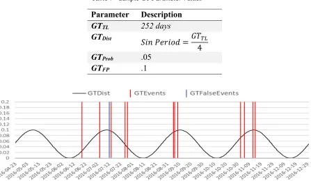
Figure 12 shows a sample GT generatedusing the parameters specified in Table 7. The total GT
set contains 252 days spanning 2016-04-23 to 2016-12-30. The sine probability curve GTDist is
shown as a black line in Figure 12. Because the curve determines the probability of an event being
generated on each given day, a clear grouping of events forms near each peak in the curve. The
GTProb of .05 results in 13 of the 252 days creating GT events, roughly 5.2% of all possible days.
The GTFP rate of .1 causes 1 of these 13 events to be classified as a false positive to be used for
Table 7 - Sample GT Parameter Values
Parameter Description
GTTL 252 days
GTDist
𝑆𝑖𝑛 𝑃𝑒𝑟𝑖𝑜𝑑 =𝐺𝑇#a 4
GTProb .05
GTFP .1
Figure 12 - Sample Event Distribution using GTProb = .05 & GTDist = Sine
Figure 13 shows another sample GT generated using the parameters shown in Table 7 but using a
uniform GTDist instead of sinusoidal. As shown by the event spacing in Figure 13, altering the
GTDist value to uniform removes the clustering of events and creates more even spacing between
event occurrences.
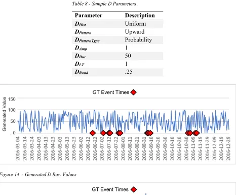
39 Figure 14 shows the raw values of a Dl set used with the GT generated in Figure 12. The data set
is generated using the GTL and DDist values shown in Table 8. The GTL value directly determines
the number of data points contained in D.
Table 8 - Sample D Parameters
Parameter Description
DDist Uniform
DPattern Upward
DPatternType Probability
DAmp 1
DDur 50
DLT 1
[image:48.612.74.540.177.563.2]DRand .25
Figure 14 - Generated D Raw Values
Figure 15 - Generated D with Pattern Applied
GT Event Times
GT Event Times
The DDistspecified creates the Uniform distribution of values between [0,100] seen in Figure 14
with no discernable pattern. These data points then have the pattern defined by DPattern, DAmp, DDur,
DLT, and DRand applied. As defined in Table 8, a DPattern value of Upward and DPatternType of
Probability result in a pattern of increasing spike likelihood until the provided event time. The
pattern is defined to be 50 data points long, with a spike amplitude of 1 standard deviation, a lead
time of 1 day, and a 25% chance of any given spike within the pattern not occurring. The D set
shown in Figure 15 has the pattern described applied, seen as higher values prior to GT events
including the negative event.
GT/D pairs generated using the method shown above determine exactly how well the method
performs when provided with different patterns and base data sets. The results