Computation of transient viscous flows using indirect
radial basis function networks
N. Mai-Duy, L. Mai-Cao and T. Tran-Cong
∗Faculty of Engineering and Surveying,
The University of Southern Queensland, Toowoomba, QLD 4350, Australia
Submitted to
CMES
, June 2006
Abstract: In this paper, an indirect/integrated radial-basis-function network (IRBFN) method is further developed to solve transient partial differential equations (PDEs)
gov-erning fluid flow problems. Spatial derivatives are discretized using one- and two-dimensional
IRBFN interpolation schemes, whereas temporal derivatives are approximated using a
method of lines and a finite-difference technique. In the case of moving interface
prob-lems, the IRBFN method is combined with the level set method to capture the evolution
of the interface. The accuracy of the method is investigated by considering several
bench-mark test problems, including the classical lid-driven cavity flow. Very accurate results
are achieved using relatively low numbers of data points.
1
Introduction
The idea of using RBFNs for solving PDEs was first proposed by Kansa (1990), where a
global multiquadric scheme was used in conjunction with point collocation to discretize
parabolic, hyperbolic and elliptic PDEs. Recently, Mai-Duy and Tran-Cong (2001a,
2001b,2003,2005) proposed an indirect RBFN method, which is based on integration
rather than differentiation, for approximating functions and their derivatives and for
solv-ing elliptic differential equations. In Kansa method, a function is first approximated by
an RBFN, and its derivatives are then obtained by differentiating such an RBFN. In the
IRBFN method, on the other hand, the highest-order derivatives in the system under
consideration are first decomposed into RBFs. Lower-order derivatives and the function
itself are then successively obtained via symbolic integrations. More recently, Mai-Cao
and Tran-Cong (2005) extended the IRBFN method for solving transient problems
gov-erned by parabolic, hyperbolic and convection-diffusion equations. This paper reports
further developments of the IRBFN method to solve transient PDEs governing viscous
flow problems. Several interpolation schemes based on 1D− and 2D−IRBFNs are
lines [e.g. Mai-Cao and Tran-Cong (2005)] and a finite-difference technique are used
for temporal discretization. For problems with moving interfaces, the present method is
combined with the level set method to capture the evolution of interfaces. A number of
benchmark test problems, namely a convection-diffusion problem governed by the Burgers
equation, the lid-driven cavity flow governed by the Navier-Stokes equations, and passive
transport problems governed by hyperbolic equations, are considered. These problems
have received much attention from the research community. The first two problems are
usually used as models for the understanding of physical flows and for the testing of new
numerical schemes in CFD, while the last problem presents several challenges associated
with the moving interfaces.
The distinguish feature of the Burgers equation is that it can be solved analytically for
many combinations of initial and boundary conditions [Fletcher (1984)] and hence, one
can evaluate the accuracy of a numerical method in a straightforward manner. In contrast,
there are no exact solutions available for the others. The lid-driven cavity flow possesses
physically unrealistic characteristics (discontinuous velocity) at the edges of the lid. This
leads to rapid changes in stress near those points, thereby making the numerical simulation
difficult. In the context of a Newtonian-fluid flow, accurate solutions for a wide range of
the Reynolds number were reported by Ghia, Ghia and Shin (1982) who used a multigrid
finite-difference (FD) scheme with very dense grids, and their results are often cited in
the literature for evaluating new viscous flow solvers. Recently, by using the Chebyshev
collocation technique, which possesses exponential convergence/spectral accuracy, for the
calculation of a regular part of the solution, and by using analytical formulae to obtain
the singular part, Botella and Peyret (1998) provided benchmark spectral results on the
flow at Re=1000. It will be shown that the 1D-IRBFN results are in closer agreement
with the spectral solutions than the FD ones. For moving interface problems, there are
two basic approaches to model the movement of the interfaces: moving-grid and
moving surface-fitted grid. This approach allows a precise representation of the interface
whereas its main drawback is the severe deformation of the mesh as the interface moves.
The second approach, which is based on fixed grids, includes capturing methods where
the moving interface is not explicitly tracked, but rather captured via a characteristic
function. For these methods, no grid manipulation (e.g. rezoning/remeshing) is needed
to maintain the overall accuracy even when the interface undergoes large deformation.
Interested readers are referred to [e.g. Floryan and Rasmussen (1989)] for a thorough
review of numerical methods for moving interfaces. In this paper, the level set method,
which belongs to fixed-grid methods, is used to capture the moving interfaces.
The remaining of the paper is organized as follows. In section 2, the IRBFN method
for solving time-dependent PDEs is described. The method is then applied to simulate
convection-diffusion, lid-driven cavity flow, and moving interface problems in sections 3,
4 and 5, respectively. Section 6 gives some concluding remarks.
2
Indirect RBFN method
2.1
Spatial discretization
A function y, to be approximated, can be represented by an RBFN as
y(x)≈f(x) =
M
X
i=1
w(i)g(i)(x), (1)
wherexis the input vector, M the number of RBFs, {w(i)}M
i=1 the set of network weights
to be found, and {g(i)(x)}M
i=1 the set of RBFs.
In the present indirect approach, RBFNs are used to represent the second-order derivatives
of a function y, i.e. ∂2y/∂x2
are then obtained by integrating those RBFNs.
2.1.1 Expressions in terms of network weights
Expressions of f and its derivatives in terms of network weights can be given by
∂2y(x)
∂x2
j
≈ ∂
2f(x)
∂x2 j = M X i=1
w[(xi)j]g[(xi)j](x), (2)
∂y(x)
∂xj
≈ ∂f(x)
∂xj
=
Z M X
i=1
w[(xi)j]g[(xi)j](x)
!
dxj = M+P
X
i=1
w[(xi)j]H[(xi)j](x), (3)
y(x) ≈ f[xj](x) =
Z M+P X
i=1
w[(xi)j]H[(xi)j](x)
!
dxj = M+Q
X
i=1
w[(xi)j]H¯[(xi)j](x), (4)
where subscript [xj] denotes the quantities resulting from the process of integration with
respect to the xj− direction, and P and Q are the numbers of centres used to represent
integration constants in the first and second derivatives, respectively (Q = 2P). Let
x(i) Ni=1 be the set of collocation points. If the above expressions are evaluated at the
chosen collocation points, one would obtain a discrete system in terms of network weights.
More details can be found in [Mai-Duy and Tran-Cong (2001a,2001b,2003)].
2.1.2 Expressions in terms of nodal function values
As an alternative approach, further manipulation of the discrete system is carried out
to convert the system into the unknown function values at collocation points. Thus,
expressions of f and its derivatives in terms of function values can be given by
∂2f(x)
∂x2
j
=hg[(1)xj](x),· · · ,0,· · · ,0,· · ·iH−1[xj]f, (5)
∂f(x)
∂xj
=hH[(1)xj](x),· · · , H[(xMj]+1)(x),· · · ,0,· · ·iH−1[xj]f, (6)
f[xj](x) =
h
¯
where f is the vector of unknown function values at the collocation points, and H[xj] is
the conversion matrix defined as
H[xj]=
¯
H[(1)xj](x(1)), · · · , H¯[(xMj]+1)(x(1)), · · · , H¯[(xMj]+P+1)(x(1)), · · ·
¯
H[(1)xj](x(2)), · · · , H¯[(xMj]+1)(x(2)), · · · , H¯[(xMj]+P+1)(x(2)), · · ·
· · · ·
¯
H[(1)xj](x(N)), · · · , H¯(M+1) [xj] (x(
N)), · · · , H¯(M+P+1) [xj] (x(
N)), · · ·
.
More details can be found in [Mai-Duy and Tran-Cong (2005)].
It can be seen that the 2D−IRBFN expressions (5)-(7) require the inversion of large
non-square matrices H[xj] of dimension N ×(M +Q). To alleviate this difficulty, one can
discretize the domain of interest using a Cartesian grid, and then apply 1D−IRBFNs to
represent the variations of the variable and its derivative along grid lines. In this case,
the inversion is conducted for a series of much smaller matrices,
H[xj]=
¯
H[(1)xj](x(1)j ) H¯
(2) [xj](x
(1)
j ) · · · H¯
(n) [xj](x
(1)
j ) x
(1)
j 1
¯
H[(1)xj](x(2)j ) H¯
(2) [xj](x
(2)
j ) · · · H¯
(n) [xj](x
(2)
j ) x
(2)
j 1
· · · ·
¯
H[(1)xj](xj(n)) H¯[(2)xj](xj(n)) · · · H¯[(xnj])(x(jn)) x(jn) 1
,
of dimensionn×(n+ 2) in which n is the number of data points along a grid line that is
parallel to the xj− direction. This leads to considerable economy in forming the system
matrix over the use of 2D-IRBFNs. As a result, much larger numbers of nodes (e.g., up to
10201 nodes in this study) can be employed. This approach is recommended for solving
complex problems, such as the lid-driven cavity flow problem, where a number of data
points is required to be large enough in order to capture complex flow patterns.
function g takes the form
g(i)(x) = qkx−c(i)k2+a(i)2, (8)
where c is the centre, a is the width and k.k denotes a Euclidean norm. The set of
collocation points is taken to be the set of centres, i.e. {x(i)}N
i=1 ≡ {c(i)}Mi=1 with N =
M, and the width a(i) is chosen to be the minimum distance from the ith centre to its
neighbours.
2.2
Temporal discretization
For problems governed by the Burgers equation and the Navier-Stokes equations, a
finite-difference scheme is used for temporal discretization, where the diffusive and convective
terms are treated implicitly and explicitly, respectively.
For moving interface problems, a method of lines is employed. The numerical solution of
the ODE system resulting from the semi-discretization of the PDE is found by means of
the fourth-order Runge-Kutta method.
3
Convection-diffusion problem
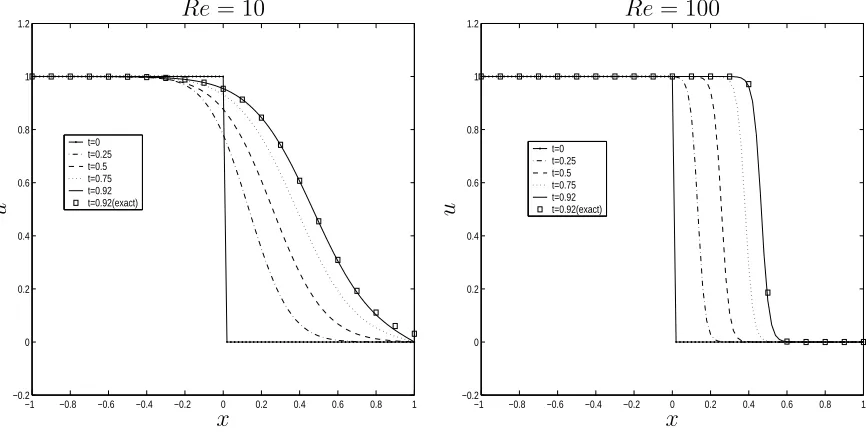
Consider a convection-diffusion problem governed by the Burgers equation. The purpose
of giving this example here is to illustrate the ability of the present method to capture
sharp gradients accurately. The method can then be used with confidence to solve more
complex problems. The Burger equation is defined as follows.
∂u ∂t +u
∂u ∂x =
1
Re ∂2u
with boundary conditions
u(−1, t) = 1, u(1, t) = 0, (10)
and initial conditions
u0(x) =u(x,0) = 1, −1≤x≤0, (11)
u0(x) =u(x,0) = 0, 0< x≤1, (12)
whereuis velocity, andRethe Reynolds number. Since it is a 1D problem, the differential
equation can be solved efficiently, without the need for converting RBF coefficients into
nodal values. The IRBFN expressions (2)-(4) can thus be used to represent the variable
and its derivatives. The space domain is discretised with 101 collocation points. Results
for the casesRe= 10 andRe= 100 are shown in Figure 1 where excelent agreement with
the exact solution [Fletcher (1984)] can be seen. The “shock” front becomes diffused at
low Revalues and remains steep with increasing Re values.
4
Lid-driven cavity flow
This is a classical benchmark problem which is suitably used here to demonstrate the
capability of the present method to simulate complex fluid flows. The lid velocity (U)
and the length of the side of the square (L) are used as reference quantities. The
non-dimensional governing equations for unsteady two-non-dimensional incompressible flow of a
Newtonian fluid in terms of the streamfunctionψand vorticityωcan be written as follows
∂ω ∂t + ∂ψ ∂x2 ∂ω ∂x1 − ∂ψ ∂x1 ∂ω ∂x2 = 1 Re
∂2ω
∂x2 1 +∂ 2ω ∂x2 2 , (13)
∂2ψ
∂x2 1 + ∂ 2ψ ∂x2 2
whereRe=U L/ν is the Reynolds number(ν: the kinematic viscosity). The vorticity and
streamfunction are defined by
ω= ∂v2
∂x1
− ∂v1
∂x2
, (15)
∂ψ ∂x1
=−v2,
∂ψ ∂x2
=v1, (16)
wherev1 and v2 are two components of the velocity vector in thex1−and x2−directions,
respectively.
The lid slides toward the right at unit velocity, while the other walls remain stationary:
ψ = 0, ∂ψ ∂x1
= 0, on x1 = 0 andx1 = 1, (17)
ψ = 0, ∂ψ ∂x2
= 0, on x2 = 0, (18)
ψ = 0, ∂ψ ∂x2
= 1, on x2 = 1. (19)
The boundary condition ψ = 0 along the boundaries can be used directly to solve (14)
for the velocity field, while one needs to derive computational boundary conditions for
the vorticity transport equation (13). Using (14) and the boundary condition ψ = 0,
expressions for the vorticity on the boundaries are reduced to ω = −∂2ψ/∂n2 (n: the
local coordinate normal to the wall). After expressing this normal second-order derivative
as a linear combination of nodal first-order derivative values, imposition of the required
boundary conditions ∂ψ/∂n is carried out. Finally, the remaining first derivative values
are written in terms of nodal streamfunction values. This process is similar to that of
a 2D-IRBFN interpolation scheme which was described in detail in [Mai-Duy and
Tran-Cong (2005)]. The present solution procedure involves the following steps
1. Guess a set of initial conditions: ω, ψ and their spatial derivatives
3. Discretize in space using 1D-IRBFN schemes:
Compute the convective term and the boundary values ofω
Solve the vorticity transport equation (13) forω
Solve Poisson equation (14) for ψ
4. Check to see whether the solution has reached a steady state
r PN
i=1
ψ(ki+1) −ψk(i)2
r PN
i=1
ψk(i+1) 2
< ǫ, (20)
wherekis the time level,ǫthe tolerance (ǫ= 10−9), andN the number of collocation
points.
5. If it is not satisfied, advance time step and repeat from step 2. Otherwise, stop the
computation and output the results.
The stability of the lid-driven cavity flow was investigated in [e.g. Poliashenko and Aidun
(1995)]. For the case of a square cavity, it was reported that the point of bifurcation
is Re = 7763, where the primary steady state becomes unstable. A range of Re =
{0,100,400,1000,3200,5000}is considered here. The computed solution at the lower and
nearest value of Re is taken to be the initial solution. The special case of Re= 0 starts
from a fluid at rest. Ten uniform grids, namely 11 ×11,21×21,· · · ,101 × 101, are
employed to study the convergence behaviour of the method. Time steps used are in the
range of 0.005−0.5. Steady-state solutions are presented in detail here, and they are
compared with some other numerical results available in the literature.
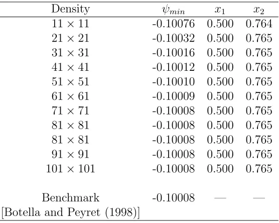
The accuracy of the method is first examined through the solution of the Stokes flow. The
governing equation for this creeping flow can be obtained from (13) by simply discarding
the nonlinear term and settingReequal to 1. The computed values of the streamfunction
Peyret (1998)] are also included to provide the basis for the assessment of the accuracy of
the present method. A very high degree of accuracy is achieved. WhenNx1 =Nx2 ≥71,
five significant digits remain unchanged.
For viscous flow (Re > 0), results concerning the extrema of the velocity profiles along
the vertical and horizontal centrelines (Re = 100 and Re = 1000), and the intensity of
the primary vortex and lower right secondary vortex (Re = 1000) are summarized in
Tables 2–5. The corresponding results obtained by the pseudospectral method [Botella
and Peyret (1998)], FDM [Ghia, Ghia and Shin (1982), Bruneau and Jouron (1990)] and
FVM [Deng, Piquet, Queutey and Visonneau (1994)] are included for comparison. The
1D-IRBFN results are in better agreement with the spectral solutions than those predicted
by FDM and FVM.
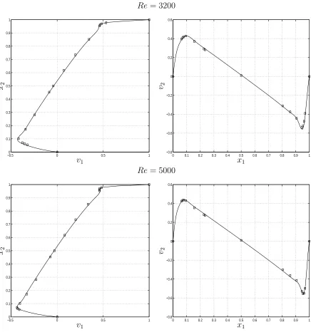
For the case of Re= 3200 and Re= 5000, velocity profiles on the vertical and horizontal
lines through the cavity geometric centre are plotted in Figure 2. They compare well with
the corresponding results of Ghia, Ghia and Shin (1982).
In addition, iso-vorticity lines of the flow for various Renumbers are shown in Figure 3.
The vorticity-contour values chosen here are the same as those in [Ghia, Ghia and Shin
(1982), Botella and Peyret (1998)], i.e. {-5, -4,-3,-2,-1,-0.5,0,0.5,1,2,3}. The plots look
reasonable when compared to those of Ghia, Ghia and Shin (1982) and Botella and Peyret
(1998).
It is worth mentioning that although the present method is global, it does not require
any special treatment for the singularity at the two corners. In contrast, when using the
spectral collocation method, it is necessary to employ a subtraction technique to remove
the leading part of the singularity.
For the simulation of the lid-driven viscous flow, the 1D-IRBFN collocation method
5
Moving interface problems
The IRBFN method is combined with the level set (LS) method in a scheme, namely
IRBFN-LS, to capture the evolution of the interface. In this work, passive transport
problems are chosen so that focus is kept on the moving interface.
5.1
Level set method
The underlying idea of the level set method is to embed a moving interface Γ as the zero
level set of a smooth (at least Lipchitz continuous) function φ(x, t) known as the level set
function [e.g. Osher and Sethian (1988)]. The moving interface is then captured at all
time by locating the set of Γ(t) for which φ vanishes. The level set function is advected
with time by a transport equation which is known as a level set equation. Usually, φ is
defined as a signed distance function to the interface. Readers are referred to [e.g. Sethian
(1999), Osher and Fedkiw (2003)] for detailed discussions on the level set method.
In the level set method, the moving interface Γ(t) which bounds an open region Ω⊂Rd
(d= 2,3) is embedded as the zero level set of a higher dimensional function φ(x, t)
Γ(t) = {x∈Rd| φ(x, t) = 0}.
Initially, φ is defined as the signed distance function from the front such that
φ(x, t) =
+d(x, t) x∈Ω+,
0 x∈Γ,
−d(x, t) x∈Ω−,
(21)
where d(x, t) represents the Euclidean distance from x to the interface, Ω− and Ω+ are
by locating the set of Γ(t) for which φ vanishes. In other words, instead of working with
the interface, one evolves the level set with the following transport equation forφ,
φt+v· ∇φ = 0, (22)
φ(x,0) =φ0, (23)
where φ0 is a given function. Whenever needed, the moving interface can be extracted
as the zero level of the level set function φ. Interested readers are referred to [e.g. Osher
and Sethian (1988), Sethian (1999), Osher and Fedkiw (2003)] for further details.
5.2
IRBFN-LS scheme
Consider a two-dimensional material interface moving with an externally generated
veloc-ity field. The IRBFN-LS scheme for capturing the interface is described by the following
steps
1. Initialize the level set function φ(x) to be the signed distance to the interface as
described by equation (21);
2. Update the externally generated velocity field using the current value of the level
set function. For Newtonian fluid flows, this involves solving the Navier-Stokes
equations by methods such as the one is discussed in section 2. For passive transport
problems, the external velocity field simply remains unchanged;
3. Solve the level set equation (22) by the method of lines for one time step using the
newly updated velocity field from step 2;
4. Re-initialize the level set function that has just been calculated from the previous
5. The interface as the zero contour of the level set function has now been advanced
one time step. Go back to step 2 for further evolution of the moving interface until
the predefined time is reached.
5.3
Initialization
At time t = 0, the signed distance function in (21) is defined as the distance from the
given collocation pointxto the initial interface curve and the sign is chosen to be positive
if the point is inside the curve, and negative if outside:
d(x,0) =±minkx−x(i)k, x(i) ∈Γ0, (24)
where Γ0 = Γ(0) is the initial interface whose discrete representation isx(i).
5.4
Method of lines
The level set equation is solved in the IRBFN framework. Using the method of lines,
one can convert the PDE (22) into a first-order initial-value system of ODEs. Spatial
derivatives, i.e. ∂φ/∂xj, are discretized by means of 2D-IRBFNs. Solving the obtained
ODE system with the initial conditions (23) yields the level set function at every data
point within the time interval of interest.
5.5
Re-initialization
While the level set functionφ is initialized as a signed distance function from the moving
interface, this is not necessarily true as time proceeds. In order to keep the numerical
evolving front Γ at each time step. The basic idea behind this scheme of re-initialization is
that given a functionφ(x) that is not a distance function, one can evolve it into a function
φ that is exact signed distance function from the zero level set of φ(x) [e.g. Sussman,
Smereka and Osher (1994)]. This is accomplished by solving the following problem to
steady state
φt=Sǫ(φ) (1− |∇φ|) (25)
φ(x,0) =φ(x), (26)
where Sǫ denotes the smoothed sign function
Sǫ(φ) =
φ
q
φ2+ǫ2
, (27)
where ǫ can be chosen to be the minimum distance from any data point to the others.
The solution procedure for (25)-(27) is similar to that of (22)-(23). It should be noted
that because the level set function is reinitialized at each time step, the steady solution
of (25) can be obtained after just a small number of iterations [e.g. Sussman, Smereka
and Osher (1994)].
5.6
Numerical examples
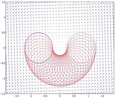
5.6.1 Solid body rotation
Consider the solid body rotation of a circular bubble of radiusr = 1 centered at (−1,0) in
a vortex flow with velocity field (v1, v2) = (−x2, x1). A half cycle of rotation is performed,
and the percentage change in area of the circle during its motion is measured. As can
with coarser point density in comparison with the mesh-based level set method [Sethian
(1999)]. Figure 4 shows the zero contours of the level set function at different points in
time during the rotation of the circle. In this figure, the computational grid consists of
41 × 41 collocation points and the time step size is chosen to be 0.0125. As can be seen
from the figure, the moving interface is well captured and reconstructed by the IRBFN-LS
method.
5.6.2 Circular bubble moving in shear flow
Consider a circular bubble of radius r = 0.15, initially centered at (0.5,0.7) moving by a
shear flow in a cavity of size [0,1]×[0,1] with the velocity field (v1, v2) defined as follows
v1 = −sin(πx1) cos(πx2), (28)
v2 = cos(πx1) sin(πx2). (29)
With such velocity field, the bubble is passively transported in forms of rotation and
stretching. The IRBFN-LS scheme is used to capture the moving interface with time
in a computational grid of 65 × 65. The time step size ∆t in the semi-discrete scheme
for solving the level set equation is chosen following the multidimensional CFL condition
[Osher and Fedkiw (2003)]
∆tmax
|v1|
∆x1
+ |v2|
∆x2
=α (30)
whereα is the CFL number, 0< α <1 and α= 0.5 for this example;|v1|and |v2|are the
absolute values of normal and tangential velocity; ∆x1 and ∆x2 are grid density in the
x1− and x2− directions, respectively. In this example, the time step size is 0.0078125.
Figure 5 shows the level set function and the moving interface as its zero level at different
time step with 5 iterations for the level set function to be a signed distance function.
Numerical experiments are carried out with the number of steps greater than 1 where the
reinitialization process is performed, and it is found that, although more computational
work is needed, reinitialization after each time step yields more stable results.
6
Concluding remarks
This paper presents further developments of the IRBFN method for the simulation of
viscous fluid flow problems. For the lid-driven cavity flow problem, numerical results
obtained show that the method yields a very high degree of accuracy. The IRBFN results
are in better agreement with the benchmark spectral solutions than those of the FDM by
Ghia, Ghia and Shin (1982). One advantage of the present method over the pseudospectral
method is that it does not require any special treatment for the singularity at the two
top corners. For moving interface problems, the present scheme combines the highly
accurate approximator coming from the IRBFN method with the advantage of the level
set method in dealing quite naturally with the moving interface as the zero contour of
a smooth function. It can be seen from the examples that the evolution of the moving
interface is captured very well by the present scheme.
ACKNOWLEDGEMENTS
L. Mai-Cao is supported by a USQ scholarship, USQ Faculty of Engineering and Surveying
scholarship and a Moldflow scholarship.
REFERENCES
1. Botella, O.; Peyret, R. (1998): Benchmark spectral results on the lid-driven cavity flow. Computers & Fluids, vol. 27(4), pp. 421-433.
incom-pressible Navier-Stokes equations. Journal of Computational Physics, vol. 89(2),
pp. 389-413.
3. Deng, G.B.; Piquet, J.; Queutey, P.; Visonneau, M. (1994): Incompressible flow calculations with a consistent physical interpolation finite volume approach.
Computers & Fluids, vol. 23(8), pp. 1029-1047.
4. Fletcher, C.A.J.(1984): Computational Galerkin Methods, Springer-Verlag, New York.
5. Floryan, J.M.; Rasmussen, H. (1989): Numerical Methods for Viscous Flows with Moving Boundary. Applied Mechanics Reviews, vol. 42(12), pp. 323–341.
6. Ghia, U.; Ghia, K.N.; Shin, C.T. (1982): High-Re solutions for incompress-ible flow using the Navier-Stokes equations and a multigrid method. Journal of
Computational Physics, vol. 48, pp. 387–411.
7. Kansa, E.J. (1990): Multiquadrics- A scattered data approximation scheme with applications to computational fluid-dynamics-II. Solutions to parabolic, hyperbolic
and elliptic partial differential equations. Computers and Mathematics with
Appli-cations, vol. 19(8/9), pp. 147–161.
8. Mai-Cao, L.; Tran-Cong, T. (2005): A Meshless IRBFN-Based Method for Transient Problems. Computer Modeling in Engineering & Sciences, vol. 7(2), pp.
149–171.
9. Mai-Duy, N.; Tran-Cong, T. (2001a): Numerical solution of differential equa-tions using multiquadric radial basis function networks. Neural Networks, vol.
14(2), pp. 185–199.
10. Mai-Duy, N.; Tran-Cong, T.(2001b): Numerical solution of Navier-Stokes equa-tions using multiquadric radial basis function networks. International Journal for
11. Mai-Duy, N.; Tran-Cong, T. (2003): Approximation of function and its deriva-tives using radial basis function networks. Applied Mathematical Modelling, vol.
27, pp. 197–220.
12. Mai-Duy, N.; Tran-Cong, T. (2005): An efficient indirect RBFN-based method for numerical solution of PDEs. Numerical Methods for Partial Differential
Equa-tions, vol. 21, pp. 770–790.
13. Osher, S.; Fedkiw, R.(2003): Level Set Methods and Dynamic Implicit Surfaces, Applied Mathematical Sciences (volume 153), Springer, New York.
14. Osher, S.; Sethian, J.A. (1988): Fronts propagating with curvature-dependent speed: algorithms based on Hamilton-Jacobi formulations. Journal of
Computa-tional Physics, vol. 79, pp. 12–49.
15. Poliashenko, M.; Aidun, C.K. (1995): A direct method for computation of simple bifurcations. Journal of Computational Physics, vol. 121, pp. 246–260.
16. Sethian, J.A. (1999): Level Set Methods and Fast Marching Methods: Evolving Interfaces in Computational Geometry, Fluid Mechanics, Computer Vision, and
Materials Science, Cambridge University Press, New York.
17. Sussman, M.; Smereka, P.; Osher, S.J. (1994): A level set approach for computing solutions to incompressible two-phase flow. Journal of Computational
Table 1: Lid-driven cavity flow, Re = 0: The minimum value of the streamfunction and its location.
Density ψmin x1 x2
11×11 -0.10076 0.500 0.764
21×21 -0.10032 0.500 0.765
31×31 -0.10016 0.500 0.765
41×41 -0.10012 0.500 0.765
51×51 -0.10010 0.500 0.765
61×61 -0.10009 0.500 0.765
71×71 -0.10008 0.500 0.765
81×81 -0.10008 0.500 0.765
81×81 -0.10008 0.500 0.765
91×91 -0.10008 0.500 0.765
101×101 -0.10008 0.500 0.765
Benchmark -0.10008 — —
Table 2: Lid-driven cavity flow, Re= 100: Extrema of the vertical and horizontal velocity profiles through the centre of the cavity.
Method Density v1min(error %) x2 v2max(error %) x1 v2min(error %) x1
Present 11×11 -0.18388(14.091) 0.484 0.14175(21.061) 0.242 -0.20870(17.770) 0.814 21×21 -0.21085(1.490) 0.464 0.17450(2.823) 0.239 -0.24734(2.545) 0.808 31×31 -0.21367(0.173) 0.459 0.17895(0.345) 0.237 -0.25278(0.402) 0.810 41×41 -0.21408(0.019) 0.458 0.17960(0.017) 0.237 -0.25368(0.047) 0.810
FVM 64×64 -0.21315(0.416) — 0.17896(0.340) — -0.25339(0.162) —
[Deng et al (1994)]
FDM(ψ−ω) 129×129 -0.21090(1.467) 0.453 0.17527(2.395) 0.234 -0.24533(3.337) 0.805 [Ghia et al (1982)]
FDM(u−p) 129×129 -0.2106 (1.607) 0.453 0.1786 (0.540) 0.234 -0.2521 (0.670) 0.813 [Bruneau and Jouron (1990)]
Benchmark -0.21404 0.458 0.17957 0.237 -0.25380 0.810
[Botella and Peyret (1998)]
Table 3: Lid-driven cavity flow,Re= 1000: Extrema of the vertical and horizontal velocity profiles through the centre of the cavity. Note that cpi.: consistent physical interpolation; stagg.: staggered.
Method Density v1min(error %) x2 v2max(error %) x1 v2min(error %) x1
Present 11×11 -0.16933(56.422) 0.244 0.14892(60.492) 0.218 -0.20926(60.298) 0.906 21×21 -0.28334(27.081) 0.254 0.25166(33.236) 0.185 -0.35962(31.771) 0.875 31×31 -0.33588(13.560) 0.192 0.32263(14.408) 0.167 -0.46097(12.543) 0.891 41×41 -0.36667(5.636) 0.177 0.35368(6.171) 0.163 -0.49844(5.434) 0.903 51×51 -0.37859(2.568) 0.174 0.36588(2.934) 0.161 -0.51356(2.565) 0.907 61×61 -0.38300(1.434) 0.174 0.37060(1.682) 0.160 -0.51939(1.459) 0.908 71×71 -0.38496(0.929) 0.173 0.37279(1.101) 0.159 -0.52199(0.966) 0.908 81×81 -0.38603(0.654) 0.173 0.37403(0.772) 0.159 -0.52344(0.691) 0.909 91×91 -0.38671(0.479) 0.173 0.37482(0.562) 0.159 -0.52436(0.516) 0.909 101×101 -0.38717(0.360) 0.172 0.37536(0.419) 0.158 -0.52499(0.397) 0.909
FVM,stagg. 128×128 -0.38050(2.077) — 0.36884(2.149) — -0.51727(1.861) — FVM,cpi. 128×128 -0.38511(0.890) — 0.37369(0.862) — -0.52280(0.812) — [Deng et al (1994)]
FDM(ψ−ω) 129×129 -0.38289(1.462) 0.172 0.37095(1.589) 0.156 -0.51550(2.197) 0.906 [Ghia et al (1982)]
FDM(u−p) 256×256 -0.3764 (3.132) 0.160 0.3665 (2.770) 0.152 -0.5208 (1.192) 0.910 [Bruneau and Jouron (1990)]
Benchmark -0.38857 0.172 0.37694 0.158 -0.52708 0.909
[Botella and Peyret (1998)]
Table 4: Lid-driven cavity flow, Re= 1000, Primary vortex: Intensities. The results obtained by the spectral method and FDM are also included for comparison.
Method Density ψmin(error %) ω(error %) x1 x2
Present 11×11 -0.05733(51.799) -1.02512(50.423) 0.574 0.581 21×21 -0.08417(29.233) -1.66318(19.566) 0.534 0.601 31×31 -0.10317(13.259) -1.87115(9.508) 0.530 0.572 41×41 -0.11242(5.482) -1.98425(4.038) 0.532 0.566 51×51 -0.11594(2.522) -2.03170(1.743) 0.532 0.566 61×61 -0.11727(1.404) -2.04909(0.902) 0.531 0.566 71×71 -0.11787(0.900) -2.05637(0.550) 0.531 0.566 81×81 -0.11819(0.631) -2.06013(0.369) 0.531 0.566 91×91 -0.11840(0.454) -2.06237(0.260) 0.531 0.566 101×101 -0.11854(0.336) -2.06396(0.183) 0.531 0.565
FDM(ψ−ω) 129×129 -0.11793(0.849) -2.04968(0.874) 0.531 0.563 [Ghia et al (1982)]
FDM(u−p) 256×256 -0.1163 (2.220) — 0.531 0.559
[Bruneau and Jouron (1990)]
Benchmark — -0.11894 -2.06775 0.531 0.565
[Botella and Peyret (1998)]
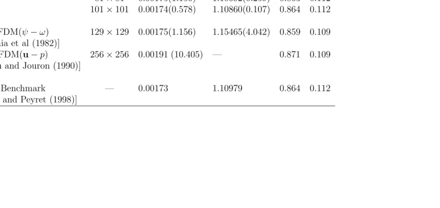
Table 5: Lid-driven cavity flow, Re= 1000, lower right secondary vortex: Intensities. The results obtained by the spectral method and FDM are also included for comparison.
Method Density ψmax(error %) ω(error %) x1 x2
Present 21×21 0.00330(90.751) 1.02999(7.191) 0.806 0.156 41×41 0.00170(1.734) 1.03920(6.361) 0.863 0.115 61×61 0.00175(1.156) 1.09919(0.955) 0.863 0.113 81×81 0.00175(1.156) 1.10692(0.259) 0.863 0.112 101×101 0.00174(0.578) 1.10860(0.107) 0.864 0.112
FDM(ψ−ω) 129×129 0.00175(1.156) 1.15465(4.042) 0.859 0.109 [Ghia et al (1982)]
FDM(u−p) 256×256 0.00191 (10.405) — 0.871 0.109 [Bruneau and Jouron (1990)]
Benchmark — 0.00173 1.10979 0.864 0.112
[Botella and Peyret (1998)]
Table 6: Solid body rotation: Comparisons between the mesh-based LSM [Sethian (1999)]
and the IRBFN-LS method on the percentage change in area att = 1.
Grid size 1st-order mesh-based LSM 2nd-order mesh-based LSM IRBFN-LS
21 ×21 51.88% 18.00% 1.6275%
−1 −0.8 −0.6 −0.4 −0.2 0 0.2 0.4 0.6 0.8 1 −0.2
0 0.2 0.4 0.6 0.8 1 1.2
t=0 t=0.25 t=0.5 t=0.75 t=0.92 t=0.92(exact)
Re= 10
x
u
−1 −0.8 −0.6 −0.4 −0.2 0 0.2 0.4 0.6 0.8 1
−0.2 0 0.2 0.4 0.6 0.8 1 1.2
t=0 t=0.25 t=0.5 t=0.75 t=0.92 t=0.92(exact)
Re= 100
x
[image:26.612.95.528.39.256.2]u
Figure 1: Burgers equation, 101 data points, ∆t = 0.001: the evolution of the “shock”
Re= 3200
−0.50 0 0.5 1
0.1 0.2 0.3 0.4 0.5 0.6 0.7 0.8 0.9 1 v1 x2
0 0.1 0.2 0.3 0.4 0.5 0.6 0.7 0.8 0.9 1
−0.8 −0.6 −0.4 −0.2 0 0.2 0.4 0.6 x1 v2
Re= 5000
−0.50 0 0.5 1
0.1 0.2 0.3 0.4 0.5 0.6 0.7 0.8 0.9 1 v1 x2
0 0.1 0.2 0.3 0.4 0.5 0.6 0.7 0.8 0.9 1
[image:27.612.93.529.110.576.2]−0.8 −0.6 −0.4 −0.2 0 0.2 0.4 0.6 x1 v2
Figure 2: Lid-driven cavity flow, 101×101 uniform grid: Velocity profiles along the vertical
and horizontal centrelines for two high values of the Reynolds number. The symbol 2
Re= 0,uniform grid = 71×71 Re= 100,uniform grid = 81×81
[image:28.612.92.534.35.485.2]Re= 1000,uniform grid = 91×91 Re= 3200,uniform grid = 101×101
Figure 3: Lid-driven cavity flow: Iso-vorticity lines of the flow for various Re numbers.
The vorticity-contour values chosen here are the same as those in [Ghia, Ghia and Shin
−1.5 −1 −0.5 0 0.5 1 1.5 −1.5
[image:29.612.113.511.186.526.2]−1 −0.5 0 0.5 1 1.5
0 0.5 1 0 0.2 0.4 0.6 0.8 1 x y
Initial zero contour
0 0.5 1 0 0.5 1 −0.5 0 0.5 1 x Initial level set function
y
Φ
0 0.5 1
0 0.2 0.4 0.6 0.8 1 x y
zero contour at t=0.666667
0 0.5 1 0 0.5 1 −0.5 0 0.5 1 x Level set function at t=0.666667
y
[image:30.612.121.508.185.521.2]Φ
Figure 5: Circular bubble moving in shear flow: Zero contour and the level set function
0 0.5 1 0 0.2 0.4 0.6 0.8 1 x y
zero contour at t=1.70833
0 0.5 1 0 0.5 1 −0.5 0 0.5 1 x Level set function at t=1.70833
y
Φ
0 0.5 1
0 0.2 0.4 0.6 0.8 1 x y
zero contour at t=2.91667
0 0.5 1 0 0.5 1 −0.5 0 0.5 1 x Level set function at t=2.91667
y
[image:31.612.118.508.185.521.2]Φ
Figure 6: Circular bubble moving in shear flow: Zero contour and the level set function


![Table 6: Solid body rotation: Comparisons between the mesh-based LSM [Sethian (1999)]and the IRBFN-LS method on the percentage change in area at t = 1.](https://thumb-us.123doks.com/thumbv2/123dok_us/282651.61146/25.612.107.518.89.135/table-rotation-comparisons-sethian-irbfn-method-percentage-change.webp)
![Figure 3: Lid-driven cavity flow: Iso-vorticity lines of the flow for various ReThe vorticity-contour values chosen here are the same as those in [Ghia, Ghia and Shin(1982), Botella and Peyret (1998)], i.e](https://thumb-us.123doks.com/thumbv2/123dok_us/282651.61146/28.612.92.534.35.485/figure-vorticity-various-vorticity-contour-values-botella-peyret.webp)