RIT Scholar Works
Theses
7-19-2019
Analyzing Binary Black hole Spacetimes
Jam Sadiq
Ph.D. Dissertation
Analyzing Binary Black hole Spacetimes
Author:
Jam Sadiq
Advisor:
Dr. Yosef Zlochower
A dissertation submitted in partial fulfilment of the requirements
for the degree of Astrophysical Sciences and Technology
in the
School of Physics and Astronomy
Ph.D. Dissertation
Analyzing Binary Black hole Spacetimes
Author:
Jam Sadiq
Advisor:
Dr. Yosef Zlochower
A dissertation submitted in partial fulfilment of the requirements
for the degree of Astrophysical Sciences and Technology
in the
School of Physics and Astronomy
Approved by
Astrophysical Sciences and Technologies
R
·
I
·
T
College of ScienceRochester, NY, USA
The Ph.D. Dissertation of Jam Sadiq has been approved
by the undersigned members of the dissertation committee as satisfactory for the degree of
Doctor of Philosophy in Astrophysical Sciences and Technology.
CHAIR, Dr. David Ross Date
ADVISOR, Dr. Yosef Zlochower Date
COMMITTEE MEMBER, Dr. Richard O’Shaughnessy Date
COMMITTEE MEMBER, Dr. Lawrence Kidder Date
With the first ever detection of gravitational waves from merging black-hole binaries by LIGO (Laser Interferometer GravitationalWave Observatory), a new era of gravitational wave astronomy was started. With its increased sensitivity, LIGO will see many more black-hole binaries in the future. To detect the gravitational waves and elucidate the properties of their sources, one needs theoretical waveform templates. These, in turn, require solving Einstein field equations, at least approximately. Approximate techniques like post-Newtonian theory and black-hole perturbation theory can produce waveforms that are accurate for certain phases of binaries evolution. Numerical relativity, on the other hand, can in principle produce accurate waveforms models for the full binary evolution. However, such simulations are computationally very expensive for the slow inspiral phase. To overcome this issue, we hybridized numerical relativity obtained by solving the Einstein field equations during the late-inspiral, plunge, and ringdown phase and post-Newtonian waveforms for the early-inspiral phase. Here we focus on hybridizing waveforms for precessing black-hole binaries. In this work we also developed a new tool to test the accuracy limits of approximate a binary black-hole spacetimes constructed using analytical approximate techniques. Our method is based on direct comparison to a numerically generated solution to the Einstein field equations.
Abstract i
Declaration v
List of published work vi
List of Tables vii
List of Figures viii
1 Introduction 1
1.1 Black Holes: Taxonomy and properties . . . 2
1.2 Gravitational Waves . . . 5
1.3 Geodesics and Curvature . . . 6
1.4 New Developments in this Thesis . . . 7
2 The General Theory of Relativity 9 2.1 Introduction to General relativity . . . 9
2.1.1 Notation . . . 10
2.2 General Relativity Formalism . . . 10
2.2.1 Space-time Manifold . . . 10
2.2.2 Scalars . . . 10
2.2.3 Vectors . . . 11
2.2.4 One-forms or Dual vectors . . . 12
2.2.5 Tensors . . . 13
2.2.6 The Metric Tensor . . . 13
2.2.7 Covariant Derivative . . . 15
2.2.8 Lie Derivative . . . 17
2.2.10 Geodesic Equation . . . 20
2.2.11 Curvature and Geodesic Deviation . . . 21
2.2.12 The Einstein Equations . . . 23
2.2.13 Black Holes . . . 25
2.2.14 Gravitational Waves on Linearized Minkowski . . . 35
3 Binary Black-hole Solution 48 3.1 Post-Newtonian Approximations . . . 49
3.1.1 Energy and Flux . . . 49
3.1.2 Taylor Waveform Approximations . . . 52
3.1.3 Post Newtonian Waveforms . . . 56
3.1.4 Precession Effects . . . 58
3.1.5 Effective One-Body . . . 60
3.1.6 Post Newtonian Errors . . . 60
3.2 Basics of Numerical Relativity . . . 61
3.2.1 The 3+1 split and the ADM Equations . . . 62
3.2.2 The Initial Data Problem . . . 66
3.2.3 Gauge Choices and Evolution Equations . . . 70
3.2.4 Numerical Methods . . . 73
3.2.5 Geodesics in 3+1 form . . . 74
3.2.6 Horizons . . . 75
3.2.7 Handling Black-hole Singularities . . . 76
3.3 Extractions of Gravitational Waves in Numerical Relativity . . . 77
3.4 CACTUS and the EINSTEIN TOOLKIT . . . 80
3.4.1 Some Important Thorns . . . 81
4 Hybridizing Precessing Waveforms for LIGO Data Analysis 82 4.1 Introduction . . . 82
4.2 Techniques . . . 85
4.2.1 Waveform Data . . . 85
4.2.2 Hybridization Procedure . . . 85
4.2.3 Accuracy of Hybrid Waveforms . . . 93
4.2.4 Results . . . 94
4.2.5 Analysis . . . 109
4.3 Conclusion and Future Directions . . . 117
5 Comparing Numerical and Analytical Spacetimes 118 5.1 Techniques . . . 121
5.1.1 Geodesic Analysis . . . 121
5.1.2 Analytic Black-Hole Binary Spacetime . . . 127
5.1.3 Reconstructing the 4-dimensional Riemann Tensor . . . 127
5.1.4 Numerical Evolutions . . . 131
5.2 Code Verification . . . 135
5.3.1 Comparing First and Second-order Matched Spacetime . . . 145
5.4 Discussion . . . 150
5.5 Conclusion . . . 152
6 Discussion 153 6.1 Summary . . . 153
6.2 Future Work . . . 155
6.2.1 Future Analysis on Hybrid Error Estimation . . . 155
6.3 Acknowledgements . . . 156
I, Jam Sadiq (“the Author”), declare that no part of this dissertation is substantially the same as any that has been submitted for a degree or diploma at the Rochester Institute of Technology or any other University. I further declare that the work in Chapters 4 and 5 are entirely mine and collaborators; Chapters 1, 2 and 3 draw heavily from the available scientific work, including textbooks and research articles. Those who have contributed scientific or other collaborative in-sights are fully credited in this thesis, and all prior work upon which this thesis builds is cited appropriately throughout the text. This thesis was successfully defended in Rochester, NY, USA on the 9th of July, 2019.
Modified portions of this dissertation have previously been published by the Author in a peer-reviewed paper appearing inPhysical Reviews D (Phys Rev D):
• Chapter 5: Comparing an analytical spacetime metric for a merging binary to a fully non-linear numerical evolution using curvature scalars.
Jam Sadiq, Yosef Zlochower, Hiroyuki Nakano
1. Comparing an analytical spacetime metric for a merging binary to a fully nonlinear numerical evolution using curvature scalars.
Jam Sadiq, Yosef Zlochower, Hiroyuki Nakano
4.1 Mismatch for all modes atMtot= 40Mfor case I. The mismatch for the`= 4, m= 4 is consistent with the large error in the PN waveform for this mode as seen in Fig. 4.6.100 4.2 Mismatch for all modes at Mtot = 40M for case II where the SEOB waveform is
hybridized with the numerical one. . . 102 4.3 Mismatch for all modes at Mtot = 40M for case II where the PN waveform is
2.1 Effective potential Veff(r) for massive particles ( = −1) and different values of L.
The positions of circular orbits, when they exist, are indicated with disks. For
L >√3rS, there exist one stable and one unstable orbit. They merge into the ISCO
forL=√3rS, whererS = 2M is the Schwarzschild radius. . . 28
2.2 Kruskal diagram of the Schwarzschild spacetime. The axes T, R indicate Kruskal-Szekeres coordinates. The two gray regions are excluded, their boundary with bold black contour indicating the central singularity r = 0. Dotted lines represent the event horizon of the black hole, and split the diagram into four regions. Region I corresponds to the original r > rS, “our universe”. Region II is the black interior
where r < rS. Region III and IV represent the “other universe” with region III
has parallel exterior with r > rS and is asymptotically flat, and region IV describe
a “white hole” with r < rS . The thick black curve is the world-line of a particle
emitted and reabsorbed by the black hole, along which three local light-cones are indicated in green. Blue lines represent r = constant world-lines, while red lines represent t= constant hyper-surfaces. . . 30 2.3 Effect of gravitational wave travelling in the z-direction on a ring of test particles.
The left panel shows a pure plus polarization, the right panel a cross polarization. The ring initially at rest (bold dashed), is warped periodically (shown with different colors) with the frequency of the gravitational wave. . . 38 2.4 Strain Sensitivity: Taken from [1]. The strain sensitivity for the LIGO Livingston
detector (L1) and the LIGO Hanford detector (H1) during O1. Also shown is the noise level for the Advanced LIGO design (gray curve) and the sensitivity during the final data collection run (S6) of the initial detectors. . . 47
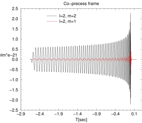
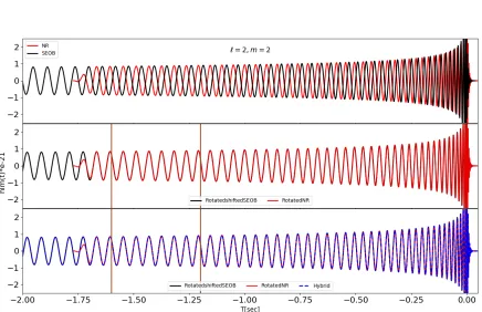
4.1 The real part of the `= 2 , m= 2 and `= 2 , m= 1 modes of a precessing binary black hole with q = 5, χ1 = (0.5,0,0) , χ2 = (0,0,0). The ` = 2 , m = 1 mode
4.2 Co-precessing frame waveform for the same system shown in Figure 4.1. Here, we show the real part of `= 2 , m = 2 and `= 2, m = 1 mode of a precessing binary black hole with q = 5, χ1 = (0.5,0,0), χ2 = (0,0,0). In the co-precessing frame the
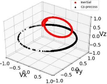
precessing binaries behaves like a non precessing binary with ` = 2 , m = 2 mode being the dominant mode of radiation. . . 90 4.3 Orbital plane for a precessing binary black hole case with q = 5, χ1 = (0.5,0,0),
χ2 = (0,0,0). The orbital plane is not aligned along the z-direction in the inertial
frame so the waveform modes behave as shown in Figure 4.1. In the co-precessing frame, the orbital plane is aligned with the z-direction and the quadrupole mode becomes the dominant mode of radiation as shown in Figure 4.2. Here, we plot the two subdominant eigenvectors of
L(ab)
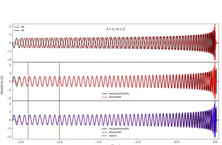
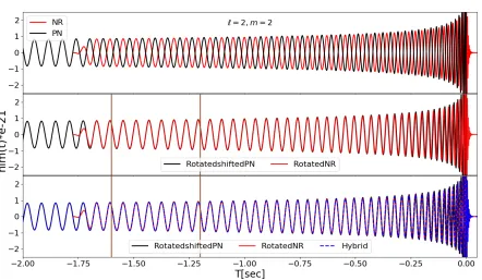
as proxies for the orbital motion. . . 91 4.4 Case I: The ` = 2, m = 2 modes of the numerical and PN waveforms. The top
panel shows the waveforms before aligning them, the middle panel shows them after alignment, and the bottom panel shows the hybrid plotted over the aligned wave-forms. The vertical lines shows the interval of hybridization. Here the total mass is
Mtot = 70M. . . 96
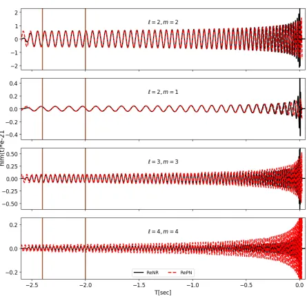
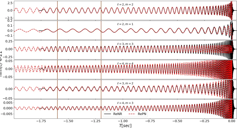
4.5 Case I: The mismatch for ` = 2, m = 2 mode between post-Newtonian-Numerical hybrid and EOB waveforms. The same hybrid waveform (suitably rescaled for dif-ferent masses) is used for all masses. We align the EOB waveform with the hybrid close to merger. The left panel shows the mismatch between the EOB and hybrid waveforms with tapering and the right panel shown mismatch without any tapering of data. There is very small difference in the mismatch with and without tapering in this case. . . 97 4.6 The PN and numerical modes for case I. These vertical lines show the hybrid interval
where the two waveforms are aligned. The ` = 3, m = 3 and ` = 4, m= 4 post-Newtonian modes show substantial amplitude errors which likely leads to the large mismatch seen in Table 4.1. These waveforms corresponds to a system withMtot =
70M. . . 98 4.7 Case II: The `= 2, m= 2 modes of the numerical and SEOBNRv4HM waveforms.
The waveforms correspond to Mtot = 70M. The top panel shows the waveforms
before aligning them, the middle panel show after alignment of two waveforms, and the bottom panel shows the hybrid plotted over the two waveforms.The vertical lines shows the interval of hybridization. . . 99 4.8 Mismatch for ` = 2, m = 2 mode between SEOB-Numerical hybrid and SEOB
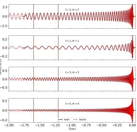
waveforms. The same hybrid waveform (suitably rescaled for different masses) is used for all masses. We align the SEOB mode after the hybrid interval. The left panel shows the mismatch of two waveforms with tapering and the right panel shown mismatch without any tapering of data. . . 100 4.9 Case II: Hybridization of higher-order modes. The vertical lines show the hybrid
in-terval where the two waveforms are aligned. The waveforms corresponds to a system withMtot= 70M. It is important to note that, unlike for the post-Newtonian
4.10 Case II: The `= 2, m= 2 mode constructed by matching the PN model waveform and numerical waveform. The waveforms corresponds to a system with Mtot =
70M. The top panel shows the waveforms before aligning them, the middle panel show after alignment of two waveforms and the bottom panel shows the hybrid over plotted to the aligned waveforms. The vertical lines shows the interval of hybridization.102 4.11 Mismatch for ` = 2, m = 2 mode between PN-Numerical hybrid and SEOB
wave-forms. We align the SEOB mode close to merger after the hybrid interval. The hybridization is performed for system with Mtot = 70M. The same hybrid
wave-form (suitably rescaled for different masses) is used for all masses. The left panel shows the mismatch of two waveforms with tapering and the right panel shown mismatch without any tapering of data. . . 103 4.12 Case II: Hybrid waveform modes constructed by matching numerical and PN
approx-imant modes. The vertical lines show the hybrid interval where the two waveforms are aligned. The waveforms corresponds to a system with Mtot = 70M. . . 103
4.13 Case III: The ` = 2, m = 1 mode constructed by matching spin-TaylorT4 approx-imant and Numerical waveforms. Both waveforms corresponds to systems with
Mtot = 70M. The top panel shows the waveforms before aligning them, the middle
panel show then after alignment, and the bottom panel shows the hybrid plotted over the two waveforms. The vertical lines shows the interval of hybridization. . . . 106 4.14 Case III: The mismatch for`= 2,m= 2 mode between Post-Newtonian-Numerical
hybrid and the longer numerical waveforms. We align the two waveforms at merger. The same hybrid waveform (suitably rescaled for different masses) is used for all masses. The left panel shows the mismatch of two waveforms with tapering and the right panel shows the mismatch without any tapering of data. Here some differences due to tapering are seen for small masses. . . 107 4.15 Case III: Hybrid waveform modes constructed by matching numerical and
post-Newtonian spin-TaylorT4 approximant modes. The vertical lines show the hybridiza-tion interval where the two waveforms are aligned. The waveforms corresponds to a system with Mtot= 70M. . . 108
4.16 The mismatch of`= 2, m= 2 mode of the Case III hybrid waveform. We choose four different intervals for the hybridization to check the accuracy of hybrid as function of length of numerical waveform used to construct the hybrid. The hybrid interval time corresponds to a system withMtot = 70M. It is clear that the longer numerical
waveform used, the smaller the mismatch. . . 110 4.17 The mismatch of ` = 2, m = 2 mode using numerical waveforms for case III with
4.18 All modes of the full precession cycle test for case III. We use a full precession cycle for the length of the hybrid interval. All the modes except the ` = 2, m= 1 mode show good alignment and this is more evident in the zoomed in plots on the lower left and right. It is important to note that we are using waveforms with total mass of Mtot= 70M. . . 113
4.19 All modes of the half precession cycle test for case III. We use a half cycle of precession for the length of the hybrid interval. A zoomed in plot is shown on the bottom. It is important to note that we are using waveforms with total mass of Mtot= 70M. . 114
4.20 All modes of the quarter precession cycle test for case III. We use a quarter precession cycle as a length of hybrid interval. A zoomed in plot is shown on the bottom. It is important to note that we are using waveforms with total mass ofMtot = 70M. . . 115
4.21 All modes of the short early hybridization interval test. We use a short interval, but at 12s (in units where the total mass is 70M). A zoomed in plot is below. It is important to note that we are using waveforms with total mass ofMtot = 70M. . . 116
5.1 Relative difference between invariant scalar for Schwarzschild and approximate Schwarzschild spacetimes. The different number of termskin Taylor series expansion gives different
approximate spacetimes. The larger thek, the better is the agreement of two space-times. For fixed k the agreement is better for large r the coordinate distance from black hole. The curvature scalars are constructed using parameters corresponding to stable circular orbits with a given energy and angular momentum for each spacetime. The relative difference of second derivative of potential also satisfy the same relations.126 5.2 The zones for the analytic metric. The large (green) circle is the outer boundary
of the near zone. Immediately inside this circle the metric is exclusively the post-Newtonian near-zone metric, while outside, it is a superposition of the near and far zone metrics. All points in the figure outside this circle are in the near-far buffer zone (the other boundary of this zone is not show). The smaller (cyan) circles denote the inner boundary of the near zone. Inside the envelope of these circles is the near-inner buffer zones. The box (orange) denotes the region inside the near-inner buffer zone where the metric is a superposition of both BH1 and BH2 inner zones, as well as the near zone. Outside the box, the metric is a superposition of the near zone metric and either one of the inner zone metrics. Finally inside the very small (magenta) circles are the two inner zones, where the metric is purely the inner zone perturbed Schwarzschild metric. . . 128 5.3 Circular geodesics in standard Schwarzschild and transformed Schwarzschild
coor-dinates. While the trajectory is gauge dependent (top), the associated curvature eigenvalues (only one shown) are not (bottom). The differences between the eigen-values (Sc) calculated in to the two gauges are consistent with roundoff errors. . . . 137 5.4 The differences between one of curvature eigenvalues(Sc) versus time from our new
5.5 The difference between one of the gauge independent curvature eigenvalue (Sc) as calculated using a fully nonlinear numerical evolution of time independent trum-pet Schwarzschild data using the EinsteinToolkit, and as calculated using the exact trumpet Schwarzschild metric with the trumpet parameterR0 =M. Here, we rescale
the differences by the ratio of the grid resolution to the fourth power. . . 138 5.6 The convergence of the one of the gauge independent curvature eigenvalues (Sc)
for a slowly time-dependent Schwarzschild trumpet. The convergence order is still fourth-order. . . 139 5.7 Second-order convergence of the gauge independent curvature eigenvalues (Sc) as
calculated using a fully nonlinear numerical evolution of Kerr data using the Einstein-Toolkit, and as calculated using the exact Kerr metric in quasi-isotropic coordinates.
. . . 140 5.8 The L2 norm of the constraints for theD= 25M configuration. Here the constraints
are calculated within the volume outside the two horizons and inside the coordinate spherer = 30M. . . 141 5.9 Separation D= 50M results. Here we plot the value of the largest (in magnitude)
curvature eigenvalue (Sc) versus time (as evolved using the numerical and analytic metric), as well as plot the coordinate position of the geodesicsin a corotating frame (i.e., one where the BH positions are nearly fixed) on the right side of each panel. The vertical lines and circles in these trajectory plots show the location of the var-ious zones described in Sec. 5.1.2. The number r0 (normalized by M) is the initial
coordinate distance of the geodesic from the nearest BH. For the geodesics close to the BHs, the noise in the numerically evolved spacetime is low compared to the magnitude of the curvature eigenvalues, the opposite is true for the farthest ones. . . 142 5.10 SeparationD= 25M andD= 20M results. Here we plot the value of the largest (in
magnitude) curvature eigenvalue (Sc) versus time (as evolved using the numerical and analytic metric), as well as plot the coordinate position of the geodesics in a corotating frame (i.e., one where the BH positions are nearly fixed) on the right side of each panel. The vertical lines and circles in these trajectory plots show the location of the various zones described in Sec. 5.1.2. The numberr0 (normalized by
5.11 SeparationD= 15M andD= 10M results. Here we plot the value of the largest (in magnitude) curvature eigenvalue (Sc) versus time (as evolved using the numerical and analytic metric), as well as plot the coordinate position of the geodesics in a corotating frame (i.e., one where the BH positions are nearly fixed) on the right side of each panel. The vertical lines and circles in these trajectory plots show the location of the various zones described in Sec. 5.1.2. The numberr0 (normalized by
M) is the initial coordinate distance of the geodesic from the nearest BH. For the geodesics close to the BHs, the noise in the numerically evolved spacetime is low compared to the magnitude of the curvature eigenvalues, the opposite is true for the farthest ones. . . 144 5.12 (Top two rows) A summary of the results. The plots show the trajectories of
the geodesics in a non-corotating frame. The color scale gives the relative differ-ences between the curvature eigenvalues (Sc) as calculated using the numerical (and smoothed by a running average) and analytic metrics. Note that the color changes from blues to reds at 10% relative difference. (Bottom two rows) Plots showing cur-vature eigenvalues as calculated using the analytical and numerical metrics, as well as a running average of the latter. There are hints here of systematic differences between the analytical and numerical results. However, as can be seen, the noise is much larger than these differences. . . 146 5.13 Curvature eigenvalues (Sc) for numerical and analytical spacetimes. For the
analyti-cal spacetime, we perturb the initial velocity of geodesics by the factors shown in the graphs. The dotted blue curve is the numerical result with velocity associated with the unperturbed analytic geodesic. As can be seen, the larger the value of the eigen-values (i.e., geodesic deviation) the larger the effect of a±10% perturbation. On the other hand, with small perturbations, we were able to find geodesics in the analytical spacetime that closely matched the dynamics (time dependence the eigenvalue) of the numerical one for geodesics farther thanr0∼10M from the BHs. . . 147
5.14 A comparison of how well the curvature eigenvalues of the second-order metric and first-order metric agree with the eigenvalues of the associated numerical metrics for the D = 50M case. The top row shows the second-order results (which were previously shown in Fig. 5.9). The bottom row shows the first-order results. Note that at larger distances from the black holes the two results are comparable, while at closer distances the second-order results are qualitatively better. . . 148 5.15 A comparison of how well the curvature eigenvalues of the second-order metric and
5.16 A comparison of how well the curvature eigenvalues of the second-order metric and first-order metric agree with the eigenvalues of the associated numerical metrics for the D = 15M case. The top row shows the second-order results (which were previously shown in Fig. 5.11). The bottom row shows the first-order results. As with theD= 20M case, there are significant differences between the analytical and numerical scalars for the first-order metric even at larger distances from the black holes. . . 149 5.17 A comparison of how well the curvature eigenvalues of the second-order metric and
1
INTRODUCTION
The contemplation of celestial things will make a man both speak and think more sublimely and
magnificently when he descends to human affairs
Cicero
It was 14th of September 2015, when two giant detectors of gravitational waves called the Laser
Interferometer gravitational wave observatory (LIGO), in the United States were undergoing final
preparation for observations, that an unexpected signal was recorded. It took several months for
careful analysis of the recorded data and what come out was one of the greatest observational
results of the century. According to the analysis, LIGO observed gravitational waves coming from
a far distant place where two black holes, both almost the mass 30 times that of the sun, merged
together to form a bigger black hole and released an enormous amount of energy equivalent to 3
times the mass of sun in the form of gravitational waves [2].
Black holes and gravitational waves are both the predictions of Einstein’s theory of general
relativity. The recorded signals of September 14th, 2015 were very close to the predictions of
Ein-stein’s theory. Not only was this an electrifying moment in science, where a theoretical prediction
similar to one 400 years ago when Galileo used a telescope and turned it to the sky to see the
universe with light. For gravitational wave astronomy, thousands of scientist worked to construct
LIGO detectors with about three decades of effort.
The detection of gravitational waves is not only a spectacular confirmation of Einstein’s theory,
but also the beginning of a new era in astrophysics. Up until now we have created a picture of
the universe from the information obtained from amazing telescopes, such as Chandra in the
X-rays, Hubble in the optical, Spitzer in the infrared, WMAP in the microwave and Arecibo in the
radio frequencies. With current and upcoming LIGO observations, as well as, gravitational wave
observations from future detectors including the LISA, Einstein telescope, Pulsar timing arrays
etc., we will be exploring the universe in a new way using an entirely new spectrum of gravitational
waves. This new type of astrophysics has an immense potential to truly revolutionize science
because gravitational waves can provide very clean information about their sources. This will help
us explore our universe’s most extreme regions which we may not be able to see with electromagnetic
waves.
1.1
Black Holes: Taxonomy and properties
Black holes are among the most mysterious astronomical objects in the universe. They are
ex-cellent theoretical laboratories that allow us to enhance our understanding of the nature of gravity.
A black hole is a region of spacetime toward which matter is drawn and from which escape is
im-possible. One of the key concept about black hole is their surface called the event horizon. Nothing,
not even light, can come out of the event horizon. Mathematically black holes can be completely
described by a few parameters. The simplest black hole is the spherically symmetric solution of
Einstein field equation known as a Schwarzschild black hole. This solution was first proposed by
Karl Schwarzschild soon after Einstein formulated theory of general relativity. The Schwarzschild
black holes are the ones which are completely described by their mass and spin. These are called
Kerr black holes. A generalization of Kerr black hole that also includes electrical charge is known
as a Kerr-Newmann black hole.
There are two general classes of black holes that are believed to exist in the universe. The ones
that are observed by LIGO are called stellar-mass black holes. They are believed to be formed by
the collapse of massive stars as they run out of fuel. The collapse causes some of the material of
star to be blown away as an explosion called a supernova. Depending on how massive the remnant
of the supernova is, the remaining matter can form a stable neutron star or completely collapse
and form a black hole. Although these black holes are supposed to have mass ranges between three
and a few 10s of solar masses. It is supposed that bigger black holes are formed by the merger of
smaller mass black holes. It is also plausible that large stellar-mass black holes formed by direct
collapse of very massive stars that were present in the early universe. The second kind of black
hole is much bigger, with the masses ranging from millions to billions of times the mass of the sun.
These are called supermassive black holes. They are believed to exist at the centers of almost every
galaxy. Our own galaxy Milky way contains a black hole of mass≈106 times heavier than the sun.
The concept of a black hole was proposed in a speculative way after Newton formulated his
theory of universal gravitation. The idea was proposed by John Mitchell [3] and independently by
Laplace [4] based on the idea of escape velocity from a gravitational field. Using the then popular
idea of light being composed of particles, and using concept of escape velocity, Mitchell speculated
about undetectable objects that are small and so massive that the escape velocity from such objects
is larger than speed of light. So they might be undetectable by direct radiation but still manifest
gravitational effects on material near them. Laplace went on to speculate that such objects may
not only exists, but even be as abundant as the visible stars. After the demise of the particle theory
It was Karl Schwarzschild [5,6] who solved Einstein’s field equations exactly for the first time
for a spherically symmetric spacetime. The result was the spacetime describing objects analogous
to what Mitchell and Laplace had speculated about. Initially, the Schwarzschild spacetime was
regarded as a mathematical curiosity rather than a representation of a real object. The reasons
for this was contentious singular terms that obscured the physical interpretation of the spacetime.
In addition, no one knew how these objects can form. Decades later in 1939, Oppenheimer and
Snyder [7] suggested that the implosion of a dying star might actually create what Schwarzschild
had found. They showed this by an analytical calculations of a dust ball undergoing a
gravita-tional collapse which leaves behind the Schwarzschild metric. These calculations describe a crude
model for stellar collapse, which was based on very simple idealized assumptions, therefore it was
still believed that such collapse could be halted in realistic astrophysical situation. One important
point of investigation was the absence of angular momentum in the Schwarzschild spacetime. It
was completely unclear how any astrophysical object, which must carry some angular momentum
could collapse to form objects described by Schwarzschild spacetime.
In 1963 Roy Kerr [8] discovered a generalization of the Schwarzschild solution with angular
mo-mentum, which shows that objects carrying angular momentum can collapsed to form black holes.
Moreover, around the same time Hawking and Penrose[9, 10] showed that general relativity
pre-dicts the creation of singularities under very generic conditions. The development of astronomical
observations and many other theoretical developments have revealed that the black holes actually
exists and Laplace was correct in his speculations. Subsequently, interest built up about another
predictions of Einstein general relativity, that of gravitational waves. It has been shown that one
of the most interesting source of gravitational waves are compact objects like black holes since the
gravitational waves emitted by the inspirals and mergers of binary black holes are the most likely
1.2
Gravitational Waves
Gravitational waves are one of the most exciting predictions of general relativity. Analogous
to electromagnetism, where accelerating charges emit electromagnetic waves, the theory of general
relativity predicts that accelerating massive bodies can produced ripples in spacetimes called
grav-itational waves. These waves carry energy and travel at speed of light. However, the intensities of
gravitational waves are exceedingly small compared to electromagnetic waves. That is why very
sophisticated, sensitive detectors with advanced technologies are required for their detections (e.g.,
LIGO). Once again, similar to electromagnetic waves which cause electrical charges to oscillate, a
passing gravitational wave will induce accelerations of test masses. More precisely, gravitational
waves stretch and squeeze the distances between test masses. Similar to electromagnetic waves,
gravitational waves have polarization states. However, they cannot be characterized by a single
polarization vector, but rather by two perpendicular directions, both also perpendicular to the
di-rection of propagation. The effect of a gravitational wave on a ring of test masses is to alternatively
stretch the ring in one of these directions and compress it in the other.
Einstein was the first to solve the equations that describe the rate of energy loss due to emission
of gravitational waves from a binary mechanical system [11]. According to his famous quadrupole
formula, the gravitational strain due to a gravitational wave is given by,
hij =
2G r
d2
dt2Qij(t−r/c), (1.1)
whereQij is the quadrupole tensors of the source. Unlike electromagnetism, there are no
gravita-tional waves due to a changing dipole moment. Just as the strength of the dipole moment governs
the efficiency of generation of electromagnetic waves, so to the strength of the quadrupole moment
control the output of gravitational waves. Einstein found that gravitational waves from realistic
astrophysical sources are so weak as to be undetectable. There was also skepticism on the existence
like black holes and neutron stars, as well as astrophysical observations like binary pulsar system
PSR 1913 + 16 [12], it become evident that gravitational waves exist.
Joseph Weber was the pioneer for the detection of gravitational waves. Although his detector,
which was based on vibrating bars, was insufficiently sensitive to actually detect astrophysical
waves, he created an interest in the field. This, and the indirect evidence of black holes and
compact objects like neutron stars and theoretical advancements gave impetus to the field. LIGO
was conceived in the 1970s and it took decades of efforts to build the two LIGO detectors in United
States. Since then LIGO detected gravitational waves from the mergers of binary compact objects,
like binary neutron stars as well as binary black holes. But gravitational waves from other sources
like pulsating neutron stars and supernova explosion will hopefully also be detected by LIGO.
There is another detectors, similar to LIGO, called Virgo in Italy that is also operational, and in
the future other detectors will be built to detect more gravitational waves. Gravitational waves
from other sources like supermassive black hole binaries as well as big bang will not be detectable
by LIGO but require more advanced detectors, such as planned space-based Laser Interferometer
Space Antenna (LISA), the Einstein telescope, A+, LIGO Voyager and Cosmic Explorer.
1.3
Geodesics and Curvature
Newton described gravity as a force that acts at a distance across the empty space between
material bodies. The Earth, for example moves in a curved orbit around the Sun because the Sun’s
gravity forces it away from its natural straight path. Einstein, on the other hand, argued that
gravity was better understood not as a force at all, but as a manifestation of spacetime geometry.
According to Einstein, the Sun’s mass distorts the geometry of spacetime in its vicinity, and the
Earth, gliding freely and without experiencing any forces, wanders along the straightest possible
path in this curved background (which is to say, it moves on a geodesic of the curved spacetime).
dimensional spacetime geometry around the star onto a 3 dimensional space.
Newtonian theory implied that a gravitational field can be detected by the tidal effects it
produces. Newton explained the tides generated on the oceans of the Earth were caused by the
gravitational field of the Moon. In Einstein’s theory tidal forces are particularly important because
they are directly related to the curvature of spacetime. This spacetime curvature is expressed in
the language of tensors using a mathematical object known as the Riemann tensor. The Riemann
tensor contains 20 independent components that encode all the geometrical information about how
the spacetime curves in different directions. It can be described by the difference in acceleration due
to gravity for two nearby particles in a gravitational field. The tidal acceleration of these particles
is proportional to the Riemann tensor and the separation between them. Given the Riemann
tensor and gravitational sources that are not too strong, the motion of falling test particles can be
computed in a routine way. In most astrophysical situations, the predictions of general relativity
and Newtonian gravity agree quite well, but there are small corrections, such as those that account
for the perihelion precession of the planet Mercury.
1.4
New Developments in this Thesis
In this work we focused on the dynamics of binary black holes. We studied the binary black
hole system using numerical and analytical techniques. In one project, we constructed hybrid
waveforms using analytical model waveforms for the early inspiral phase and available numerical
relativity waveforms for the late inspiral and merger phases of the binary black hole system. These
hybrids are important for LIGO source parameter modeling. We developed a new method for
hy-bridization which can be use to construct hybrid for generic precessing binary black hole system.
We then checked the accuracy of our hybrids in the frequency domain using standard mismatch
techniques to compared our hybrids with other models describing the same physical system. We
studied different errors in the hybrid construction that can affect the accuracy of the hybrids. We
In another project, we developed tools to compare an analytically constructed spacetime of
a binary black hole system with an equivalent numerical spacetime using timelike geodesics. We
tested the accuracy of this analytic spacetime by comparing gauge invariant quantities related
to geodesic deviation along a set of geodesics. Our method can not only be used to check the
accuracy limits of the analytical spacetime, but it can also be used to improve the accuracy of such
2
THE GENERAL THEORY OF RELATIVITY
The general theory of relativity then completed and - in contrast to the special theory - worked out by
Einstein alone without simultaneous contributions by other researchers, will forever remain the classic
example of a theory of perfect beauty in its mathematical structure.
Wolfang Pauli
2.1
Introduction to General relativity
The general theory of relativity is one of the greatest theoretical achievements of 20th century
physics. It is the theory of space, time and gravitation formulated by Einstein in 1915. At the
heart of it is the idea that gravity is the geometry of space and time. It describes gravitation in
terms of elegant mathematical structure called differential geometry. General relativity describes
the macroscopic structure of the universe. It predicts existence of exotic objects like black-holes
and neutron stars, and describes the big bang and origin of the universe. It has been verified
experimentally and so far it passes all the experimental verification. To understand and use this
theory, it is important to understand the language of differential geometry. In this chapter we will
explore important mathematical ideas needed to understand general relativity and use them to
20,21,22,23,24,25,26,27,28,29,30,31,32].
2.1.1 Notation
In this work we express tensors in both the more conventional coordinate basis and in
orthonor-mal bases. Latin indices near the beginning of the alphabet are abstract tensor indices [14], which
indicate the type of tensors involved in a calculation, as well as contraction. Latin indices near
the end of the alphabet denote coordinate-basis components of spatial tensors, while Greek letters
denote 4-dimensional spacetime components in the coordinate basis. Components of tensors in an
orthonormal basis (the first element of the orthonormal basis is always timelike) are denoted by
a Greek or Latin letter surrounded by square braces. Whether associated with coordinate bases
or orthonormal bases, Greek indices range from 0 to 3, while Latin indices near the end of the
alphabet range from 1 to 3. We use the geometric unit system, where G=c= 1.
2.2
General Relativity Formalism
2.2.1 Space-time Manifold
The mathematical structure of a spacetime is a four-dimensional manifoldM. Loosely speaking,
a manifold is a continuous space of points that may be curved globally, but locally looks like
Euclidean space Rn. Mathematically, a manifold M of dimension n is defined as a space that
can be covered by a collection of charts, that is, one-to one mappings (or coordinates) from Rn
to M. The choice of coordinates is arbitrary. A differentiable manifold is one that is continuous
and differentiable. The curved spacetime of general relativity is described in terms of differentiable
manifold.
2.2.2 Scalars
Scalar functions are functions that map points in the manifold to real or complex numbers.
point may be described byxµ= (t, x, y, z) in Cartesian coordinates can also be defined by spherical
coordinatesyµ= (t, r, θ, φ). Scalar functions are unaffected by a change of coordinates.
2.2.3 Vectors
In a curved spacetime we define vectors using directional derivatives. Let a curveγ in spacetime
be described parametrically by xα(λ), where λis a parameter. Let a function f(λ) =F(xα(λ)) be
defined on the curve. Then the derivative of f(λ) with respect toλis
df
dλ =
dxµ dλ
∂F ∂xµ =u
µ∂F
∂xµ, (2.1)
where uα = dxdλα are the components of the tangent vector u = dλd to the curve γ. That is, a directional derivative of F at a point along the curve γ is associated with a set of components
uα. Clearly the directional derivative of F itself does not depends on the coordinate system on
which it is evaluated as dλdf is same for any coordinate choice however, the components of vector
are coordinate dependent and given by,
u=uµ ∂
∂xµ =u µ∂x
0ν
∂xµ ∂
∂x0ν (2.2)
Thus the components uα of u transform as
u0α = ∂x
0α
∂xµu µ
under a coordinate transformation from xµ to x0µ, and the coordinate basis vectors ~eα = ∂x∂α
transforms as
∂ ∂x0α =
∂xµ ∂x0α
where the Jacobian matrices are the inverses of each other, i.e., satisfy
∂xµ ∂x0α
∂x0α
∂xν =
∂x0µ ∂xα
∂xα ∂x0ν =δ
µ ν
and the Kronecker delta (identity matrix)
δνµ=
1 µ=ν
0 µ6=ν
(2.3)
has same components in every coordinate system.
2.2.4 One-forms or Dual vectors
A dual vector (also called a differential form or one-form) ω = ωµ∂x
µ
∂ is a linear map which,
at each point of spacetime, takes a vector and returns a number. In other words, it takes a vector
field and returns a scalar field. The dual basis e
∼
α is defined by its operation on vector basis~e α via
e
∼
α(~e
β) =δαβ. The components of one-form transform as
ωµ0 = ∂x
ν
∂x0µων
and the dual basis e
∼
α transforms as
e
∼
0µ
= ∂x
0µ
∂xν ∼e ν
These transformations of the vectors and dual-vectors are the primary building blocks of a more
2.2.5 Tensors
The Cartesian product of an arbitrary number of dual-vectors and vectors is called a tensor. A
tensorT of rank (m
n) is expanded in a basis as
T=Tα1...αm
β1...βn ~eα1⊗...⊗~eαm⊗∼e
β1⊗...⊗e ∼
βn. (2.4)
The tensor product⊗combines tensors of rank (m
n) and (pq) into a tensor of rank mn++qp
whose
components are the direct product of the input components. Tensors are also defined by their
transformation law. The component of a tensor transform as
T0α1...αm
β1...βn =
∂x0α1
∂xγ1 ...
∂x0αm
∂xγm
∂xδ1
∂x0β1...
∂xδn
∂x0βnT
γ1...γm
δ1...δn . (2.5)
A scalar function is rank (0
0) tensor. Vectors and dual vectors are tensors of rank (10) and
(0
1), respectively. It is convenient to introduce notation for totally symmetric and anti symmetric
parts of a tensor. Tensor index symmetrization, denoted by parenthesis, is the average over all the
permutation of the order of the given indices, for example for a three index tensor
T(βγδ) = 1
3!(Tβγδ+Tγδβ+Tδβγ+Tγβδ+Tβδγ+Tδγβ) (2.6)
Tensor index anti-symmetrization, denoted by square brackets, is the average over all
permu-tation of the order of the indices, with odd permupermu-tations carrying a minus sign. For example,
T[βγδ]=
1
3!(Tβγδ+Tγδβ+Tδβγ −Tγβδ−Tβδγ−Tδγβ) (2.7)
2.2.6 The Metric Tensor
One of the most important objects in differential geometry is the rank (0
2) metric tensor g =
gαβe
∼
α⊗e
∼
u·v=gµνuµvν. The metric acts as bijective map on tangent and cotangent spaces where the vectors
and dual-vectors live. The metric is invertible with its inverse given by gµν. The metric is used
to lower indices of tensors, while its inverse raises indices. For example it transforms components
according to
ωµ=gµνων
uµ=gµνuν (2.8)
Tλνσ =gµλgρσTµνρ .
The metric is used to define the invariant line element
ds2 =gαβdxαdxβ, (2.9)
which is generalization of the Pythagorean theorem, and takes the familiar form whengαβ =δαβ.
The line element is an invariant quantity upon which all observer agrees, irrespective of the states
of motion of observer and their chosen coordinate system. For a flat spacetime, gαβ becomes the
Minkowski metric ηαβ. In Cartesian coordinates with xα = (t, x, y, z) the Minkowski metric
com-ponents areηαβ = diag(−1,1,1,1), representing a global inertial frame.
The general theory of relativity is based on the principle that, at any event, one can always
find a coordinate system where gαβ = ηαβ at that point. This is a local property of spacetime.
In other words the metric gαβ can be turned into ηαβ anywhere, but not everywhere at the same
time. This allows us to define the signature of a metric: as gµν locally corresponds to the matrix
diag(−1,1,1,1), we say that its signature is (−+ ++), which is called a Lorentzian signature. A manifold equipped with such a metric is then called a Lorentzian manifold. In contrast, a
2.2.7 Covariant Derivative
Differentiation is obviously one of the important topic in general relativity. When studying
curved spacetime, we are interested to know how things change in space and time. Differentiation
requires comparing two objects at two different points. In a curved geometry, comparing a geometric
object at two different points on manifold is not well defined. In addition, the partial derivative
of vectors and tensors do not transform like a tensor, and hence are not tensors themselves. We
want a derivative operator that does transform like a tensor. There are many different ways to
define derivative operator for curved spacetime. One of them is covariant derivative operator. It
is a linear and Leibniz map from tensor of rank (mn) to rank (nm+1). For a scalar f, the covariant
derivative reduces to ordinary derivative or partial derivative, i.e., ∇µf =∂µf.
For tensors the covariant derivative can be seen as a generalization of the partial derivative.
It appeared naturally as a way to properly take derivatives of components of vectors or tensors,
by taking into account the changes of the coordinate system when one moves from one point to
another. The underlying mathematical structure is called a connection.
The covariant derivative of a vector~v is a tensor∇µ~v, whose components are
∇µvν =vν;µ =vν,µ+ Γνρµvρ . (2.10)
The semicolon “;” and comma “,” serves as a short-hand notation for the covariant derivative and
partial derivative, respectively and the Christoffel symbols Γν
ρµ, also called connection coefficients,
are
Γνρµ = 1 2g
νσ(g
σρ,µ+gσµ,ρ−gµρ,σ). (2.11)
The Christoffel symbols are symmetric in their last indices: Γν
ρµ= Γνµρ. The connection is not a
of a dual-vector ων as
∇µων =ων;µ=∂µων−Γρµνωρ . (2.12)
More generally, the covariant derivative of a tensor is a tensor with components
Tµ1...µn
ν1...νm;ρ =T
µ1...µn
ν1...νm,ρ + Γ
µ1
σρTσ...µnν1...νm +. . .+ Γ
µn
σρTµ1...σν1...νm
−Γσν1ρTµ1...µn
σ...νm −. . .−Γ
σ νmρT
µ1...µn
ν1...σ. (2.13)
The structure is: there is a Christoffel symbol for each index of the tensor, with a plus sign if
the index is upstairs (like vectors), and a minus sign if the index is downstairs (like dual-vectors).
Just like partial derivatives, covariant derivatives are subject to the Leibniz rule with respect to
multiplication, that is
∇µ(Tνρvσ) = (∇µTνρ)vσ+Tνρ(∇µvσ) . (2.14)
Another important property of covariant derivative is that it is compatible with the metricgµν,
that is
∇ρgµν = 0 =∇ρgµν. (2.15)
This property is called metric-preservation by∇. Combined with the Leibniz rule, this means that
whenever the metric appears in a covariant derivative, it can freely be taken in or out. A particular
consequence is that indices can be freely raised and lowered when they are inside a covariant
derivative. This property is not true for simple partial derivatives. With the covariant derivatives
we can define the parallel propagation of a vector. Parallel propagation restricts the motion of a
vector along a curve or path in such a way that it remains as parallel to itself as possible at each
uµ∇µTβα11βα22...β...αmn = 0.
2.2.8 Lie Derivative
The covariant derivative requires a manifold with connection. It is possible to construct
deriva-tive for curved spacetime that utilize less structure. The Lie derivative is a coordinate invariant map from tensor of rank (m
n) to rank (mn). It measure how a tensor changes as it is moved along
the flow defined by a vector field.
Consider a vector field u on a manifold, with integral curvesxα(λ) defined by
dxα
dλ =u
α(xβ(λ)), (2.16)
where λis parameter along the curves. The curves xα(λ) form a congruence. Let Tαβ be a tensor
field which changes from Tαβ(xγ) toT
0β
α (x
0γ
) by a small displacement along the vector field uα via
active coordinate transformationxα→x0α =xα+uα then we define the Lie derivative as
LuTαβ = lim→0
Tαβ(x
0γ
)−Tα0β(x
0γ
)
. (2.17)
By Taylor expanding Tαβ(x
0γ
) aboutxγ and taking the limit, we get,
LuTαβ =uγ∂γTαβ+Tαγ∂γuβ−Tγβ∂αuγ. (2.18)
Using the symmetry of connection coefficients, the Lie derivative can be expressed using covariant
derivative as
LuTαβ =uγ∇γTαβ+Tαγ∇γuβ−Tγβ∇αuγ. (2.19)
for each index of input tensor according to above pattern. For a scalar functionf, the Lie derivative
reduces to directional derivative
Luf =uα∇αf. (2.20)
The action of Lie derivative on a vectors is naturally expressed in terms of the commutator
Luvα= [u,v]α=uβ∇βvα−vβ∇βuα (2.21)
A tensor Tαβ is said to be Lie dragged along uα if
LuTαβ = 0. (2.22)
An important application of Lie derivative is its action on the metric tensor
Lugαβ =uγ∇γgαβ +gγβ∇αuγ+gγα∇βuγ. (2.23)
If∇α is metric compatible then
Lugαβ =∇αuβ +∇βuα. (2.24)
A vector ξα is called a Killing vector if it satisfies
From the above, we see ξα is a Killing vector if
∇αξβ+∇βξα = 0. (2.26)
A Killing vector represents an isometry whereby the metric tensor is unchanged along the
direction of vector. If a metric tensor describing a spacetimes is expressed in some coordinates and
the components of metric are independent of one or more of these coordinates then there is a Killing
vector associated with that coordinate. Spacetime which are constant in time have timelike Killing
vectors whereas axisymmetric spacetimes have a space like Killing vector. Since symmetries of a
spacetime are related to conserved quantities, the existence of Killing vectors imply the existence of
conserved quantities that can be used to find the constants associated with motion along a geodesic.
For example, along a geodesic with tangent vectoruα, the quantityξαuα is unchanged
uα∇α(ξβuβ) = 0. (2.27)
2.2.9 Principle of General Covariance
Einstein’s theory of general relativity is based on the principle of equivalence which states that,
at any point in spacetime, it is always possible to construct a locally inertial coordinate system in
which the laws of special relativity are obeyed. The principle of equivalence also implies that any set
of coordinate systems are in principle suitable to describe the of laws of general relativity. Therefore,
the equations that represent these laws must remain intact with respect to any transformation of
coordinates. In other words they must be generally covariant. This led Einstein to describe the
principle of general covariance which is a mathematical expression of the generalized principle of
the theory of general relativity. The principle of general covariance states that a physical equation
holds in general gravitational field, if two conditions are met
• The equation holds in the absence of gravitation; that is, it agrees with the laws of special
and when connection coefficient Γα
βγ vanishes.
• The equation is generally covariant; that is, it preserves its form under general coordinate
transformation (xµ)→(yα)
The principle of general covariance can only be applied on a scale that is small compared with
spacetime distances typical of gravitational field, for it is only on this small scale that we are
assured by principle of equivalence of being able to construct a coordinate system in which the
effects of gravitation are absent.
2.2.10 Geodesic Equation
A curve is geodesic if it extremizes the distance between two points on a manifold. It is a
generalization of the shortest distance between two points in Euclidean space. There are two
equivalent definition of a geodesic in the Lorentzian geometry of general relativity
1. A geodesic is an extremal curveγ. More precisely, for two eventsA and B in spacetime, the
proper length or proper time between A and B along γ must be stationary with respect to
infinitesimal variations:
δs
δxµ = 0, (2.28)
with
s=
Z B
A
ds=
Z B
A
r |gµν
dxµ dλ
dxν
dλ |dλ, (2.29)
whereλ is any parameter onγ. The absolute value in the square-root is here to account for
the time-like case. In that case, s is usually denoted τ (and is the proper time between A
and B).
whereκ is any scalar function. In terms of components, this reads
uµ∇µuν = duν
dλ + Γ
ν
µρuµuρ=κuν . (2.30)
Eq. (2.30) is called thegeodesic equation.
There are three main categories of geodesics denoted by time-like, null, and space-like, where
u·uis negative, zero, or positive, respectively. It is easy to show that for a geodesic described by
Eq. (2.30), the norm of the tangent vector, N =u·u=uµuµ, withuµ= dx
µ
dλ, reads
d
dλlnN = 2κ, (2.31)
and that there exists a suitable choice for λ, called an affine parameter, such that the geodesic equation becomes uµ∇µuν = 0, that is, κ = 0. In the time-like case, proper time τ is such a
parameter while for the spacelike case it is proper distance.
2.2.11 Curvature and Geodesic Deviation
There are various equivalent ways of introducing the curvature of a manifold. One with a
particularly attractive geometric interpretation is based on the geodesic deviation equation. For any two very close geodesics, affinely parametrised bys, letξµ(s) =x2µ(s)−xµ1(s) be the separation vector. The separation vector then obeys
D2ξµ
ds2 =R
µ
νρσuνuρξσ , (2.32)
where uµ = dxdsµ is the tangent vector of one of the geodesics, and the four-index quantity Rµνρσ
represents the components of the Riemann curvature tensor. The left-hand side of eq. (2.32) can be understood as a relative “acceleration” between the two geodesics, as one moves along them.
Riemann tensor is zero. In a curved space, or spacetime, things are different as two neighbouring
geodesics can, for instance, start diverging and end up converging, like great circles on a sphere.
The Riemann tensor can also be defined by its effect on a vector v,
(∇µ∇ν− ∇ν∇µ)vσ =Rσρµνvρ , (2.33)
from which we can deduce the expression of its components which are
Rσρµν =∂µΓσρν−∂νΓσρµ+ ΓσλµΓλρν−ΓσλνΓλρµ . (2.34)
Although the Riemann tensor has, in four dimensions, 44 = 256 possible combinations of
in-dices, it enjoys a number of symmetries and identities which make this number fall to 20. These
symmetries are
Rµνρσ =−Rνµρσ , (2.35)
Rµνρσ =−Rµνσρ , (2.36)
Rµ[νρσ]= 0. (2.37)
Where, [νρσ] represents anti-symmetrization over these indices. Explicitly, we have
Rµ[νρσ]=
1
3!(Rµνρσ+Rµρσν+Rµσνρ−Rµνσρ−Rµρνσ−Rµσρν) (2.38)
= 1
3(Rµνρσ +Rµρσν +Rµσνρ), (2.39)
where the second line is obtained using the anti-symmetry of the last pair of indices. The above
relations can also be combined to show that the components of the Riemann tensor are invariant
under the exchange of the first pair and second pair of indices,
Finally, the covariant derivative of the Riemann tensor satisfies theBianchi identity
Rµ[νρσ;λ]= 0, (2.41)
where, again, [νρσ;λ] corresponds to a full anti-symmetrization over the indices (ν, ρ, σ, λ).
The Ricci tensorRµνis defined as a trace of the Riemann tensor, in the sense that its components
are
Rµν =Rρµρν , (2.42)
where we contracted the first and third indices. Using that the symmetries of the Riemann tensor,
it is easy to show that the Ricci tensor is symmetric, i.e. Rµν =Rνµ. Finally, we refer to the trace
of the Ricci tensor as theRicci scalar, which is denoted by R=Rµµ=gµλRµλ .
Another important equation is the second Bianchi identity, which is given by
Rµν −1 2δ
µ νR
;µ
= 0. (2.43)
2.2.12 The Einstein Equations
The Ricci tensor and curvature scalar are combined to form Einstein tensor Gwhich is defined
as
Gαβ =Rαβ−
1
2gαβR (2.44)
The Einstein tensor is also symmetric and due to Eq. (2.41) it satisfies
The Einstein field equations,
Gαβ =Rαβ−
1
2gαβR= 8πTαβ (2.46)
relate the spacetime curvature represented by Gαβ to the distribution of matter represented by
stress-energy tensorTαβ. Eq. (2.45) implies that the stress-energy tensor must have zero divergence,
that is
∇αTαβ = 0 (2.47)
A vacuum spacetime is defined by Tαβ = 0. Taking the trace of Eq. (2.46) we get R = 0 so that
the vacuum field equation reduces to
Rαβ = 0 (2.48)
Einstein’s equations are a non-linear system of 10 coupled partial differential equations for 10
functions (gµν) of 4 variables (xµ). Non-linearity comes from the fact that the Ricci tensor involves
the inverse of the metric, which is a non-linear operation, and products of the Christoffel symbols.
Einstein’s equation tells us that the Ricci curvature of spacetime is locally ruled by the density of
energy and momentum of matter. In the words of John Wheeler, “Spacetime tells matter how to
move; matter tells spacetime how to curve”. Another term can be added to Einstein’s equations
without changing their essential properties, i.e. the so-called cosmological constant Λ. The full Einsteins equations with cosmological constant are
Rµν−
1
2.2.13 Black Holes
A black hole is a region of spacetime that cannot communicate with the outside universe.
The boundary of this region is 3-dimensional hypersurfaces in spacetime called the surface of the
black hole or event horizon. Nothing can escape from inside of black hole, not even light. An
important feature of black hole spacetime is the presence of physical singularities. Singularities
are characterized as places where geodesics end in a finite amount of affine parameter. Physically
these are locations where tides grow without bound. Einstein’s equations continue to describe the
outside universe and inside horizon, but they break down at the singularity of the black hole. The
most general stationary black hole solution to Einstein’s field equations is that analytically known
Kerr-Newman [33] metric. This metric is uniquely specified by just three parameters: the massM,
angular momentum J and the charge Q of the black holes. The Kerr metric [8] is special case of
Kerr-Newman metric with (Q =0) which reduces to Schwarzschild metric [5, 6] with both (Q =0
and J= 0).
The Schwarzschild Solution
The Schwarzschild metric is static, spherically symmetric vacuum spacetime and describes the
field outside a spherically symmetric body. This was the first non-trivial solution of Einstein’s
field equation found by Schwarzschild [5, 6] in 1916. In Schwarzschild coordinates, the invariant
spacetime line element is given by
ds2 =−
1−2M
r
+
1 +2M
r
−1
dr2+r2dθ2+r2sin2θdφ2. (2.50)
The coordinate r is called the areal radius, with the property that two-spheres at constantr have proper area 4πr2. Birkhoff’s theorem [34] states that the Schwarzschild metric represents the unique spherically symmetric solution to the vacuum field equations. The Schwarzschild solution holds in
vacuum region of any spherical spacetime, including matter. So the space time can describe the
static observer in the vacuum exterior, is M. When the vacuum extends down to rS = 2M, the
exterior spacetime corresponds a vacuum black hole of mass M. The location rS = 2M, is the
event horizon of the black hole and sometimes called the Schwarzschild radius. The metric (2.50) is manifestly independent of t, so that we can immediately deduce the existence of a Killing vector
ξα = (∂t)α which is timelike near infinity. The metric is also independent of φ, so that there is
another Killing vector Ψα= (∂ φ)α.
In order to explore the physics of the Schwarzschild geometry, it is useful to determine the
trajectories of freely-falling particles, i.e. the geodesics of that spacetime. Suppose that there is a
geodesic whose path is xα(λ), whereλis a parameter along the curve. The vector tangent to the
geodesic is the four velocity uα = dxdλα. Then Eq. (2.27) implies that there is a conserved energy and angular momentum along the geodesic
E=−ξαuα=
1−2M
r
dt
dλ (2.51)
L=ψαuα =r2 dφ dλ
By spherical symmetry, we need only consider equatorial motion for whichθ=π/2 and dθ dλ = 0.
Substituting the conserved quantities into the line element result in an equation for radial coordinate
1 2 dr dλ 2
+Veff(r) =
E2
2 , (2.52)
where
Veff(r) =
1 2−
M
r +
L2
2r2 −
M L2
r3 , (2.53)
plays the role of an effective potential. Circular orbits (r = constant) are possible if dVeff
dr = 0.
They are stable if d2Veff
photons ( = 0), Eq. (2.52) is linear, thus it admits a single solution r = 3M. At that distance,
the gravitational field of the central massive body is strong enough to allow light to orbit around
it. However, this orbit is unstable: ddr2V2(3M) =−L2/(3M)4 <0.
For massive particles (=−1), Eq. (2.52) is quadratic, with discriminant ∆ =L2(L2−12M2) =
L2(L2−3r2
S). There are three possibilities:
1. IfL2 >3r2S, eq. (2.52) has two solutions
r±=
L rS
(L±
q
L2−3r2
S), (2.54)
corresponding to one stable (r+) and one unstable (r−) orbit. For L rS, the stable orbit r+ ≈2L2/rS corresponds to the Newtonian limit, while r−≈3M is an unstable relativistic orbit.
2. If L2 = 3r2S, the two solutions r± merge at rISCO = 6M, known as the innermost stable
circular orbit (ISCO).
3. IfL2 <3r2S, there is no circular orbit: the particle does not have enough angular momentum to keep away from the central massive object, and spirals towards the center r = 0. This is
a strictly relativistic prediction; Newtonian gravitation does not have such a feature.
The Schwarzschild metric has two singularities. The singularity in the metric at rS = 2M is a
coordinate singularity and can be eliminated by using different coordinates, while the singularity
at r = 0 is a physical spacetime singularity. In fact the curvature invariant K = RµνρσRµνρσ =
48M2/r6, also know asKretschmann scalar, clearly blows up at the origin, showing that the tidal gravitational field becomes infinite at the center of the black hole.
The coordinate singularity rS = 2M of Schwarzschild metric can be eliminated by a choice of
10−1 100 101 102 r/rS −4 −2 0 2 4 Veff ( r ) ISCO
L= 0.1rS
L=√3rS
L= 5rS
L= 8rS
Figure 2.1: Effective potentialVeff(r) for massive particles (=−1) and different values ofL. The
positions of circular orbits, when they exist, are indicated with disks. For L >√3rS, there exist
one stable and one unstable orbit. They merge into the ISCO forL=√3rS, whererS= 2M is the
Schwarzschild radius.
system in which the detailed structure of the Schwarzschild spacetime can be explored. In these
coordinates, the two angular coordinates remain unchanged, but new time and radial coordinates
are given by
T = s r rS −
1 exp r
2rS
sinh
t
2rS
, (2.55) R= s r rS −
1 exp r
2rS
cosh
t
2rS
; (2.56)
these imply, in particular,
r rS −
1 exp r rS
=R2−T2, (2.57)
tanh
t
2rS
= T
The Schwarzschild metric in Kruskal-Szekeres coordinates reads
ds2 = 4r
3
S
r exp
−r/rS
−dT2+dR2+r2dθ2+r2sin2θdφ2, (2.59)
where it is understood thatr =r(T, R) is implicitly defined by eqs. (2.55) and (2.56). This metric
is indeed has no singularity atr =rS.
An important feature of Kruskal-Szekeres coordinates is that they trivialise radial null geodesics.
Indeed, radial null curves [ ds2= 0 with dθ=dφ= 0] are simply given by
dT =±dR . (2.60)
Thus radial light rays are simply straight lines in the (T, R) plane. The full structure of the
Schwarzschild spacetime can then be represented in the Kruskal diagram Fig. 2.2, which consists of the plane (T, R). In Kruskal diagram 2.2, region I is the part which is well described by the
Schwarzschild coordinates (t, r); it represents theexterior of the black hole,r > rS. In this region, a
particle can be accelerated in order to maintainr = constant, because the associated hyperbolas are
time-like curves. It is not fundamentally different from the exterior of any massive body. A particle
following the time-like curveL upwards moves towards the centrer = 0. When the particle crosses
the lineT =R(r=rS), it enters region II, which is theinterior of the black hole. From that point,
we see that its causal future can only lead to the singularity atr = 0. The particle cannot get out
of region II, nor send any message to the exterior because that imply faster than light travel. This
is why this region is a black hole: nothing can get out of it, not even light. No information can ever
propagate from the interior (II) to the exterior (I). The surface r =rS is called the event horizon
of the black hole. Note that, in terms of the time coordinate t, the particle never actually reaches
the horizon which is not the case from the point of view of the particle itself.
The other two regions of the Schwarzschild space-time (III and IV) could not have been revealed
R T
L
r= rS, t
=+ ∞
r
=
rS , t=
−∞ t1 <
0
t2>0
r1>
rS
r2 >r
1
r = 0
r = 0
I II
[image:48.612.97.504.121.526.2]