Parametric characteristic analysis for the output frequency response function of nonlinear volterra systems

This is a repository copy of Parametric characteristic analysis for the output frequency response function of nonlinear volterra systems.

White Rose Research Online URL for this paper: http://eprints.whiterose.ac.uk/74601/

Monograph:

Jing, X.J., Lang, Z.Q. and Billings, S.A. (2006) Parametric characteristic analysis for the output frequency response function of nonlinear volterra systems. Research Report. ACSE Research Report no. 942 . Automatic Control and Systems Engineering, University of Sheffield

Reuse

Unless indicated otherwise, fulltext items are protected by copyright with all rights reserved. The copyright exception in section 29 of the Copyright, Designs and Patents Act 1988 allows the making of a single copy solely for the purpose of non-commercial research or private study within the limits of fair dealing. The publisher or other rights-holder may allow further reproduction and re-use of this version - refer to the White Rose Research Online record for this item. Where records identify the publisher as the copyright holder, users can verify any specific terms of use on the publisher’s website.

Takedown

If you consider content in White Rose Research Online to be in breach of UK law, please notify us by

Parametric Characteristic Analysis for the

Output Frequency Response Function of

Nonlinear Volterra Systems

X. J. Jing, Z. Q. Lang, and S. A. Billings

Department of Automatic Control and Systems Engineering The University of Sheffield

Mappin Street, Sheffield S1 3JD, UK

Parametric Characteristic Analysis for the

Output Frequency Response Function of

Nonlinear Volterra Systems

Xing-Jian Jing*, Zi-Qiang Lang, and Stephen A. Billings

Department of Automatic Control and Systems Engineering, University of Sheffield Mappin Street, Sheffield, S1 3JD, U.K.

{X.J.Jing, Z.Lang & S.Billings}@sheffield.ac.uk

Abstract: The output frequency response function (OFRF) of nonlinear systems is a new concept, which defines an analytical relationship between the output spectrum and the parameters of nonlinear systems. In the present study, the parametric characteristics of the OFRF for nonlinear systems described by a polynomial form differential equation model are investigated based on the introduction of a novel coefficient extraction operator. Important theoretical results are established, which allow the explicit structure of the OFRF for this class of nonlinear systems to be readily determined, and reveal clearly how each of the model nonlinear parameters has its effect on the system output frequency response. Examples are provided to demonstrate how the theoretical results are used for the determination of the detailed structure of the OFRF. Simulation studies verify the effectiveness and illustrate the potential of these new results for the analysis and synthesis of nonlinear systems in the frequency domain.

Keywords:

Parametric characteristics, Output frequency response function, Nonlinear systems

1 Introduction

of nonlinear systems (Bendat 1990, Nam and Powers 1994, Kim and Powers 1988). In Peyton-Jones and Billings (1989), Billings and Peyton-Jones (1990), and Swain and Billings (2001), the recursive algorithms for the computation of the GFRFs of discrete time, continuous time and multi-input multi-output nonlinear systems were developed, respectively. Based on these results, the output frequency characteristics of nonlinear systems were studied by Lang and Billings (1996), and some other frequency characteristics of nonlinear systems are also studied and discussed (Lang and Billings 2005, Zhang and Billings 1996). These results provide an important basis for further study of the analysis and synthesis of nonlinear systems in the frequency domain.

In Lang et al. (2006), an expression for the output frequency response, which defines an

analytical relationship between the output spectrum and the system parameters, was derived for nonlinear systems described by a polynomial form differential equation model. The result is referred to as the output frequency response function (OFRF) of nonlinear Volterra systems. The new OFRF concept reveals that for a wide class of nonlinear systems there exists a simple polynomial relationship between the output spectrum and the system parameters which define the system nonlinearities. This is an important extension of the well-known linear frequency domain relationship that the output spectrum equals to the input spectrum times the frequency response function, and provides an important basis to extend the linear frequency domain analysis and synthesis methods to the nonlinear case.

In order to determine the structure of the OFRF so as to reveal what model nonlinear parameters are available in the analytical system output frequency response description and how each of those parameters has its effect on the system output spectrum, a symbolic computation procedure was adopted for the computation of the OFRF in Lang et al. (2006). Although the symbolic computation is effective when the degrees of the system nonlinearity involved in the OFRF is not high, it is very computationally demanding and especially difficult to be used when the maximum degree of system nonlinearity considered in the OFRF is higher than 5. In order to circumvent these problems, in the present study, the OFRF of nonlinear systems is studied by a new approach referred to as the parametric characteristic analysis proposed in Jing et al (2006b), which is to study what model parameters affect a specific system response function and how those parameters have their effect on this function. By introducing a novel coefficient extraction operator, the parametric characteristics of the GFRFs are first derived and studied. Then important results about the parametric characteristics of the OFRF are developed, which explicitly reveal the analytical polynomial relationship between the system nonlinear parameters and the output spectrum, and allow the detailed structure of the OFRF to be readily determined up to any high orders without complicated symbolic computations. Examples are provided to demonstrate the application of the new results. Simulation studies verify the effectiveness and illustrate the potential of using these new results for the analysis and synthesis of nonlinear systems in the frequency domain.

Consider the following nonlinear differential equation model 0 ) ( ) ( ) , , (

1 0 , 0 1 1

1 , 1 =

∑∑ ∑

∏

∏

= = = + + = = + + M m m p K k k q p p i k k p i k k q p q p q p i i i i dt t u d dt t y d k k

c L (1)

where () ()

0 t x dt t x d k k k = =

, p+q=m,

∑

∑

∑

= = = + + ⋅ ⋅ = ⋅ K k K k K k

k, pq 0 0 pq 0

) ( ) ( ) ( 1 1

L , M is the maximum degree of

nonlinearity in terms of y(t) and u(t), and K is the maximum order of the derivative. In

this model, the parameters such as c0,1(.) and c1,0(.) are linear parameters, which

correspond to the linear terms in the model, i.e., _k

k

dt t y d ()

and _k

k

dt t u d ()

for k=0,1,…,L, and

) (⋅ pq

c for p+q>1 are nonlinear parameters corresponding to nonlinear terms in the model

of the form

∏

∏

+ + = = q p p i k k p i k k i i i i dt t u d dt t y d 1 1 ) ( ) (

, e.g., _y(t)p_u(t)q_{. p+q is called the nonlinear degree of the}

nonlinear parameterc_pq(⋅).

Under the condition that system (1) is stable at zero equilibrium, the input output relationship of the system can be approximated in the neighbourhood of the equilibrium

by a Volterra series up to maximum order N

∑

₌

∫

∫

∞

∏

∞ − = ∞ ∞ − − = N n n i i i n

n ut d

h t

y

1 1

1, , ) ( ) (

)

( L τ Lτ τ τ (2)

where h_n(τ₁,L,τ_n)is a real valued function of τ1,L,τn called the nth order Volterra kernel.

The output spectrum of the system when subject to a general input can be described as (Lang and Billings 1996)

∑

∫

∏

= − _{+ + =} = = N n n i i n n n n d j U j j H n j Y 1 1 1 1 1 ) ( ) , , ( ) 2 ( 1 ) ( ω ω ω ω σ ω ω ω π ω L

L (3)

where,

∫

∫

−∞∞ ∞ ∞ − − + +

= n n n n n

n

n j j h j d d

H ( ω1,L, ω ) L (τ1,L,τ )exp( (ω1τ1 L ωτ )) τ1L τ (4)

is the nth order GFRF. When the system is subject to a multi-tone input described by

∑

= ∠ + = K i i i

i t F

F t u 1 ) cos( )

( ω (5)

the system output spectrum can be written as (Lang and Billings, 1996):

∑

∑

= + + = = N n k k k k n n n k k n

n F F

j j H j Y 1 ₁ 1

1, , ) ( ) ( ) ( 2 1 ) ( ω ω ω ω ω ω ω ω L L

L (6)

where

{

}

⎪⎩ ⎪ ⎨ ⎧ ∈ =± ± = ∠ else 0 , , 1 , if )

( F e k K

F k

F j i

i ω ω L

ω .

∑ ∑

∑∑ ∑

∑

= = − = − = = − − + + − + = + + = ⋅ + + + − n p K k k n p n p p n q q n p K k k q n p q n k q p k q n q p q p K k k k n k n n n n p q p q p q n n n j j H k k c j j H j j k k c j j k k c j j H n L

2 , 0

1 , 1 0 , 1

1 1 , 0

1 , 1 1 , 1 , 1 1 , 0 1 1 1 1 1 1 ) , , ( ) , , ( ) , , ( ) ( ) )( , , ( ) ( ) )( , , ( ) , , ( ) ( ω ω ω ω ω ω ω ω ω ω L L L L L L L L (7)

∑

− + = + − − + + = ⋅ 1 1 1 1 1 , 1 , () ( , , ) ( , , )( ) p n i k i n i p i n i i p n p j j j j H j j H

H ω L ω ω L ω ω L ω (8a)

1 ) )( , , ( ) , ,

( 1 1 1

1 , k n n n n

n j j H j j j j

H ω L ω = ω L ω ω +L+ ω (8b)

) , , ( 1

,p n

n j j

H ω L ω in (8a) can also be rewritten as

∑ ∏

− + = = = + + + + ∑ + + = 1 1 1 1 1 1 , 1 ) )( , , ( ) , , ( p n n r r r p i k r r r r r r r n p n i p i i X X i X X

i j j j j

H j j H L L L

L ω ω ω ω ω

ω (9)

where L(n)=

∑

= + + − K k k n j j k c 0 1 1 0 , 1 1 1 ) )( (

1 ω L ω ,

∑

− = = 1 1 i x x r X .

From equations (3)(6-9), it can be seen that the direct computation of the system output spectrum involves very complicated integral and symbolic operations. Consequently the analytical relationship between the model parameters and the output frequency response can not be readily revealed from these results. In order to solve this problem, in Lang et al. (2006) an analytical relationship between the output spectrum and the system parameters was derived from these equations. The result is a polynomial function of the system nonlinear parameters as given by

∑

= N s N s N N s j j j s j j

j x x

j Y L L L 1 1 1 ( ) 1 )

( ω γ ω (10)

where x1Lxs_Nare the elements in a set consisting of all the system nonlinear parameters,

N

s

j

j1L are nonnegative integers, andγj1LjsN(ω)represents the coefficient of the term

N s N j s j x x1L

1 which is a function of frequency variable and depends on the system linear

parameters. Equation (10) was referred to as the output frequency response function (OFRF) of system (1). In order to conduct an OFRF based nonlinear system analysis and design, the first step is to determine the detailed structure of the OFRF to reveal which of the system nonlinear parameters is actually in the polynomial form expression (10) and how these parameters literally consists of the terms of the polynomial. To solve this basic problem more effectively, the OFRF is studied by using the parametric characteristic analysis in the next section.

3 Parametric characteristic analysis of the OFRF

3.1 Notations and a novel coefficient extraction operator

Define the p+qth degree nonlinear parameter vector as

)] , , ( , ), 1 , , 0 ( ), 0 , , 0 (

[ _{, , ,}

, L L L _1L4243

m q p q p q

p q

p q

p c c c K K

C

= + =

which includes all the nonlinear parameters of the form cp,q(.) with nonlinear degree p+q

in equation (1). Note that Cpq can also be regarded as a set of the (p+q)th degree

nonlinear parameters of the form cp,q(.).

Consider a series which can be written as

C C

CF c f c f c f

H = 1 1+ 2 2+L+

where the coefficients ci ∈ℜ (i=1,…, C ), ℜ denotes all the real numbers,

C=[ c1,c2,…,c_C ], C denotes the dimension of vector C, fi∈ψ (i=1,…,C ) are real or

complex valued functions,ψ denotes a set of real or complex valued scalar functions, and

F=[ f1,f2,…, fC ]

T_.

Define a Coefficient Extraction operator C

CE:ψ →ℜ such that for any

ψ

∈ +

+ +

= _{C C}

CF c f c f c f

H 1 1 2 2 L

C CF C

H

CE( )= ∈ℜ , where_ℜC

is the C -dimensional real vector space. This operator has

the following properties acting as operation rules:

(1) Reduced vectorized sum “⊕”.

CE(HC1F1+HC2F2)=CE(HC1F1)⊕CE(HC2F2)=C1⊕C2 =[C1,C′2], where C2′ is a reduced

vector of C2 which include all the elements in C2 except the same elements as those in C1.

(2) Reduced Kronecker product “⊗”.

CE(HC1F1⋅HC2F2)=CE(HC1F1)⊗CE(HC2F2)=C1⊗C2 , and “reduced” here means that

there are no repetitive components in C1⊗C2.

(3) Invariant.

(a)CE(α⋅H_CF)=CE(H_CF),∀α∈ℜwhich is not a parameter of concern; (b) CE(HCF1+HCF2)=CE(HC(F1+F2))=C

(4) Unitary. ∀HCFis not a function of ci for i=1…n, CE(HCF)=1.

Obviously, when there is a unitary 1 in CE(HCF), there is a constant term in the

corresponding series HCF which has no relation with the coefficients ci (for

i=1…n).

(5) Inverse. CE-1(C)=HCF.

(6) ( ) ( )

2 2 1

1F CF

C CE H

H

CE ≈ if the elements of C1 are the same as those of C2, where “≈”

means equivalence, i.e., both series are in fact the same result.

From property (6), it is known that the CE operator is also commutative and associative

considering the order of cifi in the series has no effect on the value of a function series

HCF, for instance, CE(HC1F1 +HC2F2)=C1⊕C2 ≈CE(HC2F2 +HC1F1)=C2⊕C1 . It should be

emphasized that the coefficient extractor CE is a coefficient oriented operator. That is,

operator. Hence, the operation result is different for different purposes. Moreover, for

convenience, let ()

(*)⋅

⊗ and ()

(*)⋅

⊕ denote the multiplication and addition in terms of the

reduced Kronecker product “⊗” and vectorized sum “⊕” for the non-repetitive (.)’s

satisfying (*), respectively; and denote pq pq pq

k

i C =C ⊗ ⊗C

⊗

=1 L simply as

k pq

C .

According to the definition of the CE operator, the parametric characteristics of the GFRFs can be obtained by directly replacing the operations “+” and “.” in the recursive

algorithm (7-9) with “⊕ ” and “⊗”respectively, and neglecting the corresponding

complex valued functions of frequency which are independent of the nonlinear parameters. In order to derive the parametric characteristics of the OFRF, the GFRFs are first investigated by the parametric characteristic analysis in the following section.

3.2 Parametric characteristics of the GFRFs

This is the first step to derive the parametric characteristics of the OFRF.

3.2.1 Derivation of the GFRFs’ parametric characteristics

The parametric characteristics of the GFRFs of equation (1) can be obtained by directly applying the CE operator as follows.

Applying the CE operator to equation (7) for the nonlinear parameters yields

⎟ ⎟ ⎠ ⎞ ⎜ ⎜ ⎝ ⎛ + ⎟ ⎟ ⎠ ⎞ ⎜ ⎜ ⎝ ⎛ + ⎟ ⎟ ⎠ ⎞ ⎜ ⎜ ⎝ ⎛ = ⋅ =

∑ ∑

∑∑ ∑

∑

= = − = − = = + −+ + − − = + + + − n p K k k n p n p p n q q n p K k k q n p q n k q p k q n q p q p K k k k n k n n n n n n p q p q p q n n n j j H k k c CE j j H j j k k c CE j j k k c CE j j H n L CE j j H CE

2 , 0

1 , 1 0 , 1

1 1 , 0

1 , 1 1 , 0 , 1 1 , 0 1 1 1 1 1 1 1 ) , , ( ) , , ( ) , , ( ) ( ) )( , , ( ) ( ) )( , , ( )) , , ( ) ( ( )) , , ( ( ω ω ω ω ω ω ω ω ω ω ω ω L L L L L L L L L )) , , ( ( )) , , ( ( )) , , ( ( ) , , ( )) , , ( ( ) , , ( ) , , ( 1 , 0 , 2 1 , , 1 1 1 , 0 1 , 1 0 , 0 , 2 1 , 1 , 0 , 1 1 1 1 , 0 0 , 1 1 1 n p n p n p q n p q n q p q n p n q n n p n p p K k k n p q n p q n q p q p K k k q n p n q n n K k k j j H CE C j j H CE C C j j H CE k k c j j H CE k k c k k c p q p n ω ω ω ω ω ω ω ω L L L L L L L ⊗ ⊕ ⊕ ⊗ ⊕ ⊕ ⊕ = ⊗ ⊕ ⊕ ⊕ ⊗ ⊕ ⊕ ⊕ ⊕ ⊕ = = − − − = − = = = − − + = − = − = = +

which can be rewritten as

⎟ ⎠ ⎞ ⎜ ⎝ ⎛_{⊕ ⊗ ⋅} ⊕ ⎟ ⎠ ⎞ ⎜ ⎝ ⎛_{⊕⊕ ⊗ ⋅} ⊕ = = − − = − = ( ()) ( ()) )) , , (

( _{,0 ,}

2 , , 1 1 1 , 0

1 p np

n p p q n q p q n p n q n n

n j j C C CE H C CE H

H

CE ω L ω (11a)

Applying the CE operator to equation (8) yields

which can be written as )) ( ( )) ( ( )) (

( _{, 1}

1 1

, ⋅ = ⊕ ⋅ ⊗ − − ⋅

+ −

= i n ip

p n

i p

n CE H CE H

H

CE (11b)

Applying the CE operator to equation (9) yields

) , , ( ( ) ) )( , , ( ( )) , , ( ( 1 1 1 1 1 , 1 n n k n n n n n j j H CE j j j j H CE j j H CE ω ω ω ω ω ω ω ω L L L L = + + =

which can be written as

))) ( ( )) (

(H_n,1 ⋅ =CE H_n ⋅

CE (11c)

Moreover, by applying the CE operator to equation (9), (11b) can also be written as

)) ( ( )) ( ( 1 1 1 , 1 ⋅ ⊗ ∑ ⊕ = ⋅ = + − = = i i p r p i p n n r r r p

n CE H

H CE

L (11d)

Note that when n=1, H1(jω1)has no relation with the nonlinear parameters of equation (1),

thus it follows from the definition of the CE operator thatCE(H₁(⋅))=1. From equations

(11a-d), the nonlinear parameters involved in the nth order GFRF Hn(jω1,L,jωn) can be

determined recursively. The following example is provided to make an illustration of the results above.

Example 1. Computation of the parametric characteristics of the GFRFs of system (1) up

to 3rd order according to (11a-d). For n=2,

(

)

) 12 ( )) ( ( )) ( ( 1 )) ( ( 1 )) ( ( )) ( ( )) ( ( )) ( ( )) , ( ( 0 , 2 1 , 1 2 , 0 1 1 0 , 2 1 , 1 2 , 0 2 1 1 2 1 0 , 2 1 , 1 2 , 0 2 , 2 0 , 2 1 , 1 1 , 1 2 , 0 , 2 0 , 2 2 , 2 , 2 1 1 1 2 , 0 2 1 2 2 1 C C C H CE H CE C C C H CE C C C H CE C H CE C C H CE C H CE C C j j H CE i i r i r r r p p p p q q p q p q ⊕ ⊕ = ⋅ ⊗ ⋅ ⊗ ⊕ ⊗ ⊕ = ⎟ ⎟ ⎟ ⎠ ⎞ ⎜ ⎜ ⎜ ⎝ ⎛ ⋅ ⊗ ∑ ⊕ ⊗ ⊕ ⊗ ⊕ = ⋅ ⊗ ⊕ ⋅ ⊗ ⊕ = ⋅ ⊗ ⊕ ⊕ ⋅ ⊗ ⊕ ⊕ ⊕ = = == = − − = = L ω ω

where equations (11cd) are used in the third and fourth equalities. From the definition of the CE operator, equation (12) implies that there exist complex valued functions of frequencies f_2i(jω₁,jω₂), i=1,2,3,…,D2, where D2 is the dimension of CE(H2(jω1,jω2)),

such that

[

]

(

)

( , ) ) ( ) ( ) ( )) , ( ( ) , ( 2 1 2 0 , 2 1 , 1 2 , 0 2 21 21 2 1 2 2 1 2 2 ω ω ω ω ω ω j j f C C C f f f j j H CE j j

H D T

⋅ ⊕ ⊕ = ⋅ ⋅ ⋅ ⋅ = L (13)

where

[

]

T

D f f f j j

f ( , ) () () () 2 2 21 21 2 1

(

)

(

)

(

)

(

)

(

) (

)

(

) (

)

) 14 ( ) ( ) ( )) ( ( )) ( ( )) ( ( )) ( ( )) ( ( )) ( ( )) ( ( )) ( ( )) ( ( )) ( ( )) ( ( )) ( ( )) ( ( )) ( ( )) ( ( )) ( ( )) ( ( )) ( ( )) ( ( )) ( ( )) , , ( ( 0 , 3 2 0 , 2 2 , 0 0 , 2 2 , 1 1 , 2 0 , 2 1 , 1 2 1 , 1 2 , 0 1 , 1 3 , 0 0 , 3 0 , 2 1 , 1 2 , 0 0 , 2 2 , 1 1 , 2 0 , 2 1 , 1 2 , 0 1 , 1 3 , 0 0 , 3 2 0 , 2 2 , 1 1 , 2 2 1 , 1 3 , 0 1 1 1 0 , 3 1 2 0 , 2 1 2 , 1 1 1 1 , 2 2 1 , 1 3 , 0 3 , 3 0 , 3 2 , 3 0 , 2 1 , 1 2 , 1 2 , 2 1 , 2 1 , 2 1 , 1 3 , 0 , 3 0 , 3 2 , 3 , 3 1 2 1 3 , 0 , 3 0 , 3 2 , 3 , 3 1 2 1 3 , 0 3 1 3 C C C C C C C C C C C C C C C C C C C C C C C C C H CE C C C H CE C C H CE H CE H CE C H CE H CE C H CE C H CE H CE C H CE C C H CE C H CE C H CE C H CE C H CE C C H CE C H CE C C H CE C H CE C C j j H CE p p p p q q p q p q p p p p q q p q p q ⊕ ⊕ ⊗ ⊕ ⊕ ⊕ ⊗ ⊕ ⊕ ⊗ ⊕ = ⊕ ⊕ ⊕ ⊗ ⊕ ⊕ ⊕ ⊕ ⊕ ⊗ ⊕ = ⊕ ⋅ ⊗ ⊕ ⊕ ⊕ ⋅ ⊗ ⊕ = ⋅ ⊗ ⋅ ⊗ ⋅ ⊗ ⊕ ⋅ ⊗ ⋅ ⊗ ⊕ ⋅ ⊗ ⊕ ⋅ ⊗ ⋅ ⊗ ⊕ ⋅ ⊗ ⊕ = ⋅ ⊗ ⊕ ⋅ ⊗ ⊕ ⋅ ⊗ ⊕ ⋅ ⊗ ⊕ ⋅ ⊗ ⊕ = ⋅ ⊗ ⊕ ⊕ ⋅ ⊗ ⊕ ⊕ ⊕ = ⋅ ⊗ ⊕ ⊕ ⋅ ⊗ ⊕ ⊕ ⊕ = = − − = = = − − = = ω ω L

In the derivation of equation (14), equations (11cd) and (12) and the properties of CE are used. Obviously, there also exists a complex valued function

vector

[

]

T

D f f f j j j

f ( , , ) () () () 3 3 31 31 3 2 1

3 ω ω ω = ⋅ ⋅ L ⋅ of frequencies such that

) , , ( )) , , ( ( ) , ,

( _{1 2 3 3 1 2 3 2 1 2 3}

3 jω jω jω CE H jω jω jω f jω jω jω

H = ⋅ (15)

Equations (12) and (14) show clearly that which of the nonlinear parameters in equation

(1) contribute to the 2nd and 3rd order GFRFs and how the contributions are made. In

addition, equations (13) and (15) indicate that the GFRFs can be expressed as an explicit polynomial function of the system nonlinear parameters.

From the definition of the CE operator and the parameter characteristics of the GFRFs in (11), the following proposition can be established following the discussions in Example 1.

Proposition 1. There exists a complex valued function vector f_n(jω₁,L,jω_n)with an appropriate dimension, such that

(

( , , )

)

( , , )

) , ,

( _{1 n n 1 n n 1 n}

n j j CEH j j f j j

H ω L ω = ω L ω ⋅ ω L ω (16)

whereCE

(

Hn(jω1,L,jωn)

)

can be recursively determined from (11a)-(11d).

Remark 1. It should be noted that f_n(jω₁,L,jω_n)in equation (16) is a function of frequency variablesω1,L,ωnand the linear parameters c10(.) and c01(.), but is independent

of the nonlinear parameters in CE

(

Hn(jω1,L,jωn)

)

.

Proposition 1 provides an explicit analytical relationship between the nonlinear parameters and the GFRFs of system (1) by the parametric characteristic analysis of the GFRF. From this explicit analytical expression of the GFRFs in Equation (16), the parametric characteristics of the OFRF of system (1) can be obtained.

3.2.2 Some further results

characteristics of the GFRFs and to simplify the computation ofCE

(

H_n(jω₁,L,jω_n)

)

, the following results are established.

Lemma 1. The elements of CE(Hn(jω1,L,jωn)) include the nonlinear parameters in C0n

and all the non-repetitive monomial functions (of the nonlinear parameters) in

k kq

p q

p q p

pq C C C

C ⊗ ₁₁ ⊗ ₂₂⊗L⊗ , where the subscripts satisfy p q p q n k

k

i

i i + = +

+

+

∑

=1

)

( ,

k n q p_i+ _i ≤ −

≤

2 , 0≤k≤n−2, 2≤ p+q≤n−k and 1≤ p≤n−k.

Proof. See Appendix.

Remark 2. Lemma 1 provides detailed information about what nonlinear parameters are

involved in the analytical description of the GFRF Hn(jω1,L,jωn) and how these

parameters have their effects on the GFRFs. It also provides a very effective method for the determination of CE

(

Hn(jω1,L,jωn)

)

. It is easy to directly write out the elements of

(

H_n(j ₁, ,j _n)

)

CE ω L ω according to Lemma 1 without any recursive computations. This can

be performed by a simple computer program which will be discussed in a future study.

To demonstrate the significance of Lemma 1, consider the following example.

Example 2. Consider the 2nd order GFRF. Then p q p q k

k

i

i i+ = +

+

+

∑

=

2 ) ( 1

, 0≤k≤2−2 =0.

Therefore, all the subscript combinations for k=0 is (p,q): (0,2);(1,1),(2,0), corresponding to the nonlinear parameters: C0,2, C1,1, C2,0. Thus CE

(

H2(jω1,jω2)

)

= C0,2+C1,1+C2,0. This is

consistent with equation (12).

Consider the 3rd order GFRF, thenp q p q k

k

i

i i + = +

+

+

∑

=

3 ) ( 1

, 0≤k≤3−2=1.

When k=0, the involved nonlinear parameters are C0,3, C1,2, C2,1, C3,0;

When k=1,p+q+ p₁+q₁ =3+1=4, which has the following non-repetitive combinations

(p,q,p1,q1 ):(1,1,2,0), (1,1,1,1),(1,1,0,2),(2,0,0,2),(2,0,2,0)

thus the involved nonlinear parameter monomials are:

C1,1oC2,0, C1,1oC1,1, C1,1oC0,2, C2,0oC0,2, C2,0oC2,0

HenceCE

(

H₃(jω₁,L,jω₃)

)

= C0,3+C1,2+C2,1+C3,0+ C1,1oC2,0+C1,1oC1,1+C1,1oC0,2

+C2,0oC0,2 +C2,0oC2,0

The result is consistent with Equation (14).

The following result follows from Lemma 1, which can be used to simplify equation (11a).

Lemma 2. CE(Hn,p(⋅))=CE

(

Hn−p+1(⋅)

)

Proof. See the Appendix.

Proposition 2. For n>1,

⎣ ⎦

) 17 ( ))

( ( ))

( (

)) , , ( (

1 0

, 2 1

2 0 , 1

, 1 1 1 , 0

1

⎟ ⎟ ⎠ ⎞ ⎜

⎜ ⎝ ⎛

⋅ ⊗

⊕ ⊕ ⊕ ⎟ ⎠ ⎞ ⎜

⎝

⎛_{⊕⊕ ⊗ ⋅}

⊕

= − +

+

= +

− − −

= −

= p n p

n

p n p

q n q

p q n

p n q n

n n

H CE C

C H

CE C C

j j H

CE ω L ω

where ⎣ ⎦⋅ is to take the integer part.

Proof. Using Lemma 2, equation (11a) now can be written as (n>1)

⎟ ⎠ ⎞ ⎜

⎝

⎛_{⊕ ⊗ ⋅}

⊕ ⎟ ⎠ ⎞ ⎜

⎝

⎛_{⊕⊕ ⊗ ⋅}

⊕

= _{− +}

= +

− − −

= −

= ( ()) ( ())

)) , , (

( _{,0 1}

2 1

, 1 1 1 , 0

1 p n p

n p p

q n q

p q n

p n q n n

n j j C C CE H C CE H

H

CE ω L ω

Considering the symmetry of the last term of this equation, Equation (17) follows. This completes the proof.

Obviously, it is much simpler to determine the parametric characteristics of the GFRFs by equation (17) than by equations (11a-d).

3.3 Parametric characteristics of the OFRF

From the parametric characteristics of the GFRFs above, the following results for the output spectra of system (1) can be achieved.

Proposition 3. Assume system (1) is stable at zero equilibrium and can be approximated by a Volterra series of a finite order. Then there exist a series of complex valued function

vectors Fn(jω)(n=1,2,…,N) of frequency variableω with appropriate dimensions such

that the OFRF of system (1) can be expressed as

(

)

[

_T

]

T

N T

T n

n N

n CE H j j F j F j F j

j

Y( ) ( ₁, , ) ₁( ) ₂( ) ( )

1 ω ω ω ω ω

ω L ⎟⋅ L

⎠ ⎞ ⎜

⎝ ⎛ ⊕ =

= (18)

where

∫

∏

= +

+ =

− ⋅

=

ω ω ω

ω

σ ω ω

ω π

ω

n

n

i

i n

n n

n f j j U j d

n j F

L

L

1 1

1

1 ( , , ) ( )

) 2 (

1 )

( . If the input of system (1) is

the multi-tone signal (5), then there exist a series of complex valued function vectors

) (jω

Fn (n=1,2,…,N) of frequency variableωwith appropriate dimensions, such that the

OFRF of system (1) can be expressed as

(

)

T

T N T

T k

k n N

n CEH j j F j F j F j

j Y

n ⎥⎦

⎤ ⎢⎣

⎡ ⋅ ⎟ ⎠ ⎞ ⎜

⎝ ⎛ ⊕ =

= ( , , ) ( ) ( ) ( )

)

( 1 2

1 ω1 ω ω ω ω

ω L L (19)

where

∑

= + +

⋅ =

ω ω ω

ω ω

ω ω

ω

n k k

n

n k k

k k

n n

n j f j j F F

F

L

L L

1

1

1, , ) ( ) ( ) (

2 1 )

( . The parametric characteristics of

the OFRF is

(

( , , )

)

)) (

( ₁

1 n n

N

n CEH j j

j Y

CE ω ω L ω

= ⊕

= (20)

(

)

(

)

(

)

(

)

[

_T

]

T

N T T n n N n N n n n n N n n i i n n n n n N n n i i n n n n n j F j F j F j j H CE j F j j H CE d j U j j f n j j H CE d j U j j f j j H CE n j Y n n ) ( ) ( ) ( ) , , ( ) ( ) , , ( ) ( ) , , ( ) 2 ( 1 ) , , ( ) ( ) , , ( ) , , ( ) 2 ( 1 ) ( 2 1 1 1 1 1 1 1 1 1 1 1 1 1 1 1 1 1 ω ω ω ω ω ω ω ω σ ω ω ω π ω ω σ ω ω ω ω ω π ω ω ω ω ω ω ω ω ω L L L L L L L L L ⋅ ⎟ ⎠ ⎞ ⎜ ⎝ ⎛ ⊕ = ⋅ = ⋅ ⋅ = ⋅ ⋅ = = = = − + + = = = − + + = =

∑

∑

_∫

∏

∑

_∫

∏

Following a similar procedure, equation (19) can be obtained for the OFRF of equation (1) actuated by a multi-tone input function in (5). Moreover, (20) is obvious from equations (18-19). This completes the proof.

Equations (18) and (19) show that the OFRF of system (1) can now be expressed as an explicit polynomial function of the nonlinear parameters, and the specific form of the OFRF of system (1) is completely defined by its parametric characteristics in (20). Because the parametric characteristics defined by equation (20) can be readily determined using Proposition 2 or Lemma 1, the parametric characteristic analysis for the OFRF of system (1) provides an effective approach to the determination of the OFRF.

In order to demonstrate the use of Proposition 3, consider the following example.

Example 3. Consider a nonlinear system,

) ( 296 16000 240 2 2 3

1x c x x u t

c x x

x&=− − &− & − & +

& (21)

subject to a sinusoidal input u(t)=100sin(8.1t). (21) is a simple case of system (1) with

M=3, K=2, c₁₀(2)=240, c₁₀(1)=296, C₁₀(0)=16000, c30(111)=c1, c30(110)=c2, c01(0)=−1,

and all other parameters are zero.

In system (21), only nonlinear parameters in C30 are not zero, i.e.,

[

30 30

] [

2 1

]

30 c (110) c (111) c c

C = =

In this case, equation (17) can be rewritten as (n>1)

⎣ ⎦ )) ( ( )) , , (

( 2 _{,0 1}

1 2 0 ,

1 = ⊕ ⊕ ⊗ − + ⋅

+

= p n p

n

p n n

n j j C C CE H

H

CE ω L ω (22)

Since only C30 is not zero, it can be shown from equation (22) that

0 )) , , (

(H_2k j ₁ j _n =

CE ω L ω and k

n

k j j C

H

CE( 2 +1( ω1,L, ω ))= 30, for k=1,2, 3,…

From equation (20) in Proposition 3,

(

)

⎣ 12⎦

30 3 30 2 30 30 1

1 ( , , ) 1

)) (

( −

= = ⊕ ⊕ ⊕ ⊕ ⊕

⊕

= n n N

N

n CEH j j C C C C

j X

CE ω ω L ω L (23a)

so that

⎣ ⎦ T

T N T T N j F j F j F C C C C j

X ⎟⋅_⎢⎣⎡ _⎥⎦⎤

⎠ ⎞ ⎜

⎝

⎛ _{⊕ ⊕ ⊕ ⊕ ⊕}

= 1 − ( ) ( ) ( )

)

( 2 1 2

1 30 3 30 2 30

30 ω ω ω

ω L L (23b)

where

⎣

N−1₂

⎦

_{is to take the integer part. From (23)CE(X(jω))can be readily obtained. For}

⎣ ⎦₌

⊕ ⊕ ⊕ ⊕ ⊕

= −12

30 3

30 2 30 30 1 )) (

(X j C C C CN

CE ω L [1,c2,c1,c22,c2c1,c12,c23,c22c1,c2c12,c13,c24,

c23c1,c22c12,c2c13,c14,c25, c24c1, c23c12,c22c13,c2c14,c15]. (23c)

Therefore an explicit analytical expression for the OFRF X(jω)in terms of the system

nonlinear parameters c1 and c2 are obtained as given by (23b-c).

3.4 A numerical method for the determination of the OFRF

As discussed in the last section, the detailed polynomial structure of the OFRF can be determined definitely by the parametric characteristic analysis. Based on structure of the OFRF, a numerical method can be used to determine the OFRF of system (1).

Denote the dimension ofCE(Y(jω)) as DY which can be known from the parametric

characteristics of the OFRF. Letφ [a₁ a₂ a ] CE(Y(jω))

Y

D =

= L where ai, i=1…DY, are the

monomial functions of the system nonlinear parameters known from the OFRF structure using Proposition 3, and

[

]

[

_T

]

T

N T

T

D j F j F j F j

h j

h j h j h

Y ( )

~ )

( ~ ) ( ~ ) ( )

( ) ( )

( ω = 1 ω 2 ω L ω = 1 ω 2 ω L ω

where F~_i(jω)=Fi(jω)when the input is a general input and ( ) ( )

~ _{ω ω}

j F j

Fi = i when the input

is a muli-tone signal. Then equation (18) can be rewritten as

) ( )

(jω φ h jω

Y = ⋅ (24)

In order to obtain the OFRF, h(jω) in (24) is needed to be determined. This can be

achieved by following a numerical method in Lang et al. (2006). The basic idea of this

method is to perform simulations or experimental tests on the system under NY (>0)

different sets of nonlinear parameters φ1, φ 2, …φ NY to obtain NY output frequency

responses of the system Y(jω)1, Y(jω)2, …Y(jω)NY for a considered input excitation.

Thus from (24), it is known that

Y

Y j

h =

⋅

Φ ( ω) (25)

where

⎥ ⎥ ⎥ ⎥ ⎥

⎦ ⎤

⎢ ⎢ ⎢ ⎢ ⎢

⎣ ⎡

=

⎥ ⎥ ⎥ ⎥ ⎥

⎦ ⎤

⎢ ⎢ ⎢ ⎢ ⎢

⎣ ⎡

=

⎥ ⎥ ⎥ ⎥ ⎥

⎦ ⎤

⎢ ⎢ ⎢ ⎢ ⎢

⎣ ⎡

= Φ

Y Y

Y Y

Y

Y Y

Y D

Y

N D N

N

D D

N Y j

j Y

j Y

Y

a a

a

a a

a

a a

a

) (

) (

) (

, 2

1

1 1

2 22

12

1 21

11 2

1

ω ω ω

φ φ φ

M M

O M M

L L

M . Consequently h(jω) can be

obtained as

(

)

Y

T T

Y j

h( ω)= Φ ⋅Φ−1⋅Θ ⋅ (26) Therefore, the OFRF of system (1) can be well determined. From this explicit analytical expression of the system output frequency response, the analysis and synthesis of system (1) in the frequency domain can be conducted. These will be illustrated in a simulation study in the next section.

5 Simulation studies

y=16000x+296x&+c₁x&3 +c₂x&2x (27) which is a more complicated function of the system states.

Since it can be shown that CE(Y(jω))=CE(X(jω))(Jing, et. al. 2006a), the theoretical

results for X(jω)still hold for Y(jω). Therefore, it follows from Example 3 that

(

)

⎣ 12⎦

30 3

30 2 30 30 1

1 ( , , ) 1

)) (

( −

= = ⊕ ⊕ ⊕ ⊕ ⊕

⊕

= n n N

N

n CE H j j C C C C

j Y

CE ω ω L ω L (28a)

and

⎣ ⎦ T

T N T

T N

j F j

F j F C

C C C j

Y ⎟⋅_⎢⎣⎡ _⎥⎦⎤

⎠ ⎞ ⎜

⎝

⎛ _{⊕ ⊕ ⊕ ⊕ ⊕}

= 1 − ( ) ( ) ( )

)

( 2 1 2

1 30 3

30 2 30

30 ω ω ω

ω L L (28b)

For clarity of illustration, consider the simpler case of c2=0, i.e., C30=c1. When N=21, it

can be shown from (28ab) that

[

10

]

1 3

1 2 1 1 1 )) (

(Y j c c c c

CE ω = L

and

[

]

[

]

T

j h j

h j h c c

c c j

h j

Y( ) ( ) 1 10 ₁( ) ₂( ) ₁₁( )

1 3

1 2 1

1 ω ω ω

ω φ

ω = ⋅ = L ⋅ L

In order to determine h(jω)in the above equation, simulation studies are carried out for

11 different values of c1 as c1=0.5,50,100,500, 800,1200, 1800, 2600, 3500, 4500, 5000,

to produce 11 corresponding output responses. The FFT results of these responses at the

system driving frequency ω0=8.1 rad/s were obtained as

YY=[(3.355387229685395e+002)-9.144123368552089e+000i,

(3.311400634432650e+002)-8.791324203084603e+000i, (3.270304131496312e+002)-8.453482697096458e+000i, (3.020996757260479e+002)-6.232073185455284e+000i, (2.889224705331136e+002)-4.937579404570077e+000i, (2.753247618357106e+002)-3.513785421406298e+000i, (2.599814606290563e+002)-1.799344961942028e+000i, (2.449407272303421e+002)-7.146831574203648e-003i, (2.322782654921158e+002)+1.587748875652816e+000i, (2.213884644417550e+002)+3.022652971105967e+000i, (2.168038059608033e+002)+3.644341792781596e+000i]

Then from (26), h(jω₀)was determined as

) (jω0

h =[3.355850061999765e+002 +9.147787717329777e+000i,

-0.09260545518186 - 0.00733079515829i

7.802545290190465e-005 +4.196941358069068e-006i -8.171412395831490e-008 -3.472552369765044e-009i 7.983194136013857e-011 +2.975659825236403e-012i -6.014819558373321e-014 -2.095287675780629e-015i 3.139462445085954e-017 +1.055716258995395e-018i -1.065920417366710e-020 -3.515136904764629e-022i 2.214834610655676e-024 +7.220197982843919e-026i -2.536564081104798e-028 -8.209302192093296e-030i 1.219975622824295e-032 +3.929425356306088e-034i].

Consequently, the OFRF of nonlinear system (27) at frequencyω0was obtained as

[

]

[

]

T

j h j

h j h c c

c c j

Y( ) 1 10 ₁( ₀) ₂( ₀) ₁₁( ₀) 1

3 1 2 1 1

0 ω ω ω

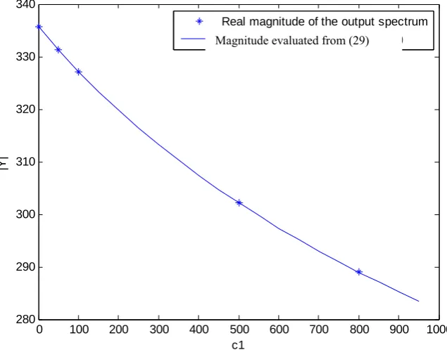
From equation (29), the effect of the nonlinear parameter c1 on the system output

frequency response at frequency ω0 can readily be analysed. Figure 1 shows a

comparison of the magnitudes of the output spectrum evaluated by (29) and their real

values under different values of the nonlinear parameter c1. Clearly, an excellent match is

achieved. Furthermore, the frequency domain analysis and design of system (21) to achieve a desired output response y(t) can now be conducted from (29). The idea is

straightforward. Given a desired output spectrum Y* at frequency ω0 , the nonlinear

parameter c1 can be optimized using (29) such that the difference |Y(jω0)-Y

[image:16.595.134.452.267.516.2]

*

| can be made as small as possible.

0 100 200 300 400 500 600 700 800 900 1000 280

290 300 310 320 330 340

c1

|Y

|

Real magnitude of the output spectrum Magnitude valued by equation (26)

Figure 1 Relationship between the output spectrum and nonlinear parameter c1

6

Conclusions

The parametric characteristics of the output frequency response function (OFRF) of nonlinear systems described by a polynomial form differential equation model have been established. Based on these results, the OFRF with its detailed structure for this class of nonlinear systems can explicitly be determined up to any high orders. The OFRF concept provides an important basis for the analysis and design of nonlinear systems in the frequency domain. The present study solves an important and basic problem associated with the OFRF based nonlinear system analysis and design. The results should be considerately significant for the frequency domain study of nonlinear systems, and for the application of the nonlinear system frequency domain approach in engineering practice.

Acknowledgement

The authors gratefully acknowledge the support of the Engineering and Physical Science Research Council, UK and the EPSRC-Hutchison Whampoa Dorothy Hodgkin Postgraduate Award, for this work.

Appendix: Proofs

PROOF OF LEMMA 1:

C0,n is the first term in equation (11a). For clarity, consider a simpler case that there is

only output nonlinearities in (11a), then (11a) is reduced to only the last term of equation

(11a), i.e., ( ()) ( ())

1 1

1 0 , 2 ,

0 ,

2 1

⋅ ⊗

∑ ⊕ ⊗ ⊕ = ⋅ ⊗

⊕

= + −

== =

= i

i p

r p i p n

n r

r r p n p p n p

n

p C CE H C L CE H . Note that

(

()

)

1 1 1 1

⋅ ⊗

∑ ⊕

= == + −

i

i p

r i

p

n r

r r

p n

H CE

L includes all the combinations of (r1,r2,…,rp) satisfying r n

p

i i =

∑

=1

,

1

1≤ri ≤n−p+ , and 2≤p≤n . Moreover, CE( H1(⋅) )=1 since there are no nonlinear

parameters in it, and any repetitive combinations have no contribution. Hence,

(

()

)

1 1 1 1

⋅ ⊗

∑ ⊕

= =

= + −

i

i p

r i

p

n r

r r

p n

H CE

L must include all the possible non-repetitive combinations of (r1,r2,…,rk)

satisfying r n p k

k

i

i = − +

∑

=1

, 2≤r_i ≤n−p+1 and 1≤k≤ p. So does CE(Hn(jω1,L,jωn)). Each

of the subscript combinations corresponds to a monomial of the involved nonlinear

parameters. Thus, including the term Cp,0 and considering the range of each variable (i.e.,

ri, p, and k), CE(Hn(jω1,L,jωn)) must include all the possible non-repetitive monomial

functions of the nonlinear parameters of the form Cp0⊗Cr10 ⊗Cr20⊗L⊗Crk0satisfying

k n r p

k

i

i = +

+

∑

=1

, 2≤ri ≤n−k , 0≤k≤n−2 and 2≤ p≤n−k . When the other types of

nonlinearities are considered, just extend the results above to a more general case that the nonlinear parameters appear in the formCpq⊗Cp1q1⊗Cp2q2 ⊗L⊗Cp_kq_k and the subscripts

satisfy p q p q n k

k

i

i i + = +

+

+

∑

=1

)

( , 2≤ p_i +q_i ≤n−k , 0≤k ≤n−2 , 2≤ p+q≤n−k and

k n p≤ −

≤

1 . Hence, the proposition is proved.

PROOF OF LEMMA 2:

According to Lemma 1, CE

(

Hn−p+1(⋅)

)

includes all the terms Cp1q1 ⊗Cp2q2⊗L⊗Cpkqksatisfying

k p n k p n q p

k

i

i

i + = − + + − = − +

∑

=

1 1 )

( 1

, 2≤ p_i+q_i ≤n−p−k+2, 0≤k−1≤n−p−1,

(

)

(

)

(

)

(

)

⎟ ⎟ ⎟

⎠ ⎞

⎜ ⎜ ⎜

⎝ ⎛

⋅ ⊗ ∑

⊕ ⊕ ⋅ =

⋅ ⊗ ∑

⊕ =

= =

= − +

− =

= = + −

) ( )

( )

( )

, , (

1 1 1

1 1 1 1

,

1

1 i

i p i

i p

r i

p

n r

r r

p n p

n r

i p

n r

r r

p n n p

n j j CEH CEH CEH

H CE

L L

L ω

ω

Considering all the possible effective combinations of (r1,r2,…,rp) in the second term on

the right of the second equality in this equation, which can be written as

(

( ()) ( ()) ( ())

)

2 1

1 2

⋅ ⊗

⊗ ⋅ ⊗

⋅ ∑

⊕

′

′ + − =

= −

q

i p

r r

r q p n r

r r

p n

H CE H

CE H

CE L

L

(A1)

As shown in the proof of Lemma 1, all the terms in (A1) satisfy

q p n q p n r

q

i

i = − + + ′− = − + ′

∑

′

=

1 1 1

, 2≤ri ≤n−p−(q′−1)+1 and 0≤q′−1≤p , i.e.,

q p n q p

q

i

i

i + = − + ′

∑

′

=1

)

( , 2≤ pi +qi ≤n−p−q′+2, and 0≤q′−1≤n−p−1 corresponding to

the nonlinear parameter monomialsCp1q1⊗Cp2q2 ⊗L⊗Cp_q′q_q′ . Moreover, it can be noted

from equation (11a) that the variable p>0. This implies that there at least is one pi>0 from

the nature of the recursive computation of equation (11a). Hence, the terms in (A1) are included inCE

(

Hn−p+1(⋅)

)

. This completes the proof.

References

Bendat J.S.(1990), Nonlinear System Analysis and Identification from Random Data, New York: Wiley.

Boyd S. and Chua L. O.(1985), Fading memory and the problem of approximating nonlinear operators with Volterra series, IEEE Trans. Circuits Syst., vol. CAS-32, 1150--1161, Nov.

Bedrosian E. and Rice S. O., (1971), The output properties of Volterra systems driven by harmonic and Gaussian inputs. Proceedings of the Institute of Electrical and Electronics Engineering, 59, 1688-1707

Corduneanu C. and Sandberg I.W. (2000), Volterra equations and applications. Singapore: Gordon and breach science publishers

George D.A.(1959), Continuous nonlinear systems, Technical Report 355, MIT Research Laboratory of Electronics, Cambridge, Mass. Jul. 24.

Jing X.J., Lang Z.Q. and Billings S.A. (2006a). Frequency Domain Analysis Based Nonlinear Feedback Control for Suppressing Periodic Disturbance. The 6th World Congress on Intelligent Control and Automation, June 21-23, Dalian, China (A full version was submitted to Inter. Jour. Of Cont.)

Jing X.J., Lang Z.Q. Billings S.A. and Tomlinson G. R. (2006b). The parametric characteristic of frequency response functions for nonlinear systems. To appear in International Journal of Control, Vol. 79, No. 12, Dec 2006, 1552-1564

Khalil H. K. (2002), Nonlinear systems, Third edition, New York: Prentice Hall Press Kim K.I., and Powers E.J., (1988), A digital method of modelling quadratic nonlinear

systems with a general random input. IEEE Trans. Acoustics, Speech and Signal Processing, 36, 1758-1769

Lang Z.Q., and Billings S.A.(2005), Energy transfer properties of nonlinear systems in the frequency domain, International Journal of Control, Vol 78, 345-362

Lang Z.Q., Billings S.A., Yue R. and Li J.(2006), Output frequency response functions of nonlinear Volterra systems, Research Report No 902, Department of ACSE, University of Sheffield. (A full version was provisionally accepted by Automatica) Nam S.W. and Powers E.J.(1994), Application of higher-order spectral analysis to

cubically nonlinear-system identification, IEEE Transactions on Signal Processing,

42(7), pp. 1746 1765, Jul.

Peyton-Jones J.C. and Billings S.A.(1989). Recursive algorithm for computing the frequency response of a class of nonlinear difference equation models. International Journal of Control, Vol. 50, No. 5, 1925-1940.

Rugh W.J. (1981), Nonlinear System Theory: the Volterra/Wiener Approach, Baltimore, Maryland, U.S.A.: Johns Hopkins University Press.

Sastry S. (1999), Nonlinear system: analysis, stability, and control. New York: Springer Swain A.K. and Billings S.A. (2001). Generalized frequency response function matrix for

MIMO nonlinear systems. International Journal of Control. Vol. 74. No. 8, 829-844 Zhang H. and Billings S.A. (1996), Gain bounds of higher order nonlinear transfer