Nonlinear output frequency response functions of MDOF systems with multiple nonlinear components

This is a repository copy of Nonlinear output frequency response functions of MDOF systems with multiple nonlinear components.

White Rose Research Online URL for this paper: http://eprints.whiterose.ac.uk/74590/

Monograph:

Peng, Z.K., Lang, Z.Q. and Billings, S.A. (2006) Nonlinear output frequency response functions of MDOF systems with multiple nonlinear components. Research Report. ACSE Research Report no. 930 . Automatic Control and Systems Engineering, University of Sheffield

[email protected] https://eprints.whiterose.ac.uk/

Reuse

Unless indicated otherwise, fulltext items are protected by copyright with all rights reserved. The copyright exception in section 29 of the Copyright, Designs and Patents Act 1988 allows the making of a single copy solely for the purpose of non-commercial research or private study within the limits of fair dealing. The publisher or other rights-holder may allow further reproduction and re-use of this version - refer to the White Rose Research Online record for this item. Where records identify the publisher as the copyright holder, users can verify any specific terms of use on the publisher’s website.

Takedown

If you consider content in White Rose Research Online to be in breach of UK law, please notify us by

Nonlinear Output Frequency Response

Functions of MDOF Systems with Multiple

Nonlinear Components

Z K Peng, Z Q Lang, and S A Billings

Department of Automatic Control and Systems Engineering The University of Sheffield

Mappin Street, Sheffield S1 3JD, UK

Nonlinear Output Frequency Response

Functions of MDOF Systems with Multiple

Nonlinear Components

Z.K. Peng, Z.Q. Lang, and S. A. Billings

Department of Automatic Control and Systems Engineering, University of Sheffield Mappin Street, Sheffield, S1 3JD, UK

Email: [email protected]; [email protected]; [email protected]

Abstract: In engineering practice, most mechanical and structural systems are modeled as Multi-Degree-of-Freedom (MDOF) systems. When some components within the systems have nonlinear characteristics, the whole system will behave nonlinearly. The concept of Nonlinear Output Frequency Response Functions (NOFRFs) was proposed by the authors recently and provides a simple way to investigate nonlinear systems in the frequency domain. The present study is concerned with investigating the inherent relationships between the NOFRFs for any two masses of nonlinear MDOF systems with multiple nonlinear components. The results reveal very important properties of the nonlinear systems. One significant application of the results is to detect and locate faults in engineering structures which make the structures behave nonlinearly.

1 Introduction

If a differential equation or discrete-time model is available for a nonlinear system, the GFRFs can be determined using the algorithm in [4]~[6]. However, the GFRFs are much more complicated than the FRF. GFRFs are multidimensional functions [7][8], which can be difficult to measure, display and interpret in practice. Recently, the novel concept known as Nonlinear Output Frequency Response Functions (NOFRFs) was proposed by the authors [9]. The concept can be considered to be an alternative extension of the FRF to the nonlinear case. NOFRFs are one dimensional functions of frequency, which allow the analysis of nonlinear systems in the frequency domain to be implemented in a manner similar to the frequency domain analysis of linear systems and which provide great insight into the mechanisms which dominate important nonlinear behaviours.

The present study is concerned with the analysis of the inherent relationships between the NOFRFs for any two masses of MDOF systems with multiple nonlinear components. The results reveal, for the first time, very important properties of the nonlinear systems, and can be applied to detect and locate faults in engineering structures which make the structures behave nonlinearly.

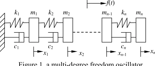
[image:4.612.172.430.397.507.2]

2. MDOF Systems with Multiple Nonlinear Components

Figure 1, a multi-degree freedom oscillator

A typical multi-degree-of-freedom oscillator is shown as Figure 1, the input force is added on the Jth mass.

If all springs and damping have linear characteristics, then this oscillator is a MDOF linear system, and the governing motion equation can be written as

) (t F Kx x C x

M&&+ &+ = (1) where

⎥ ⎥ ⎥ ⎥

⎦ ⎤

⎢ ⎢ ⎢ ⎢

⎣ ⎡

=

n m m

m

M

L M O M M

L L

0 0

0 0

0 0

2 1

is the system mass matrix, and

mn kn mn-1

m2

m1 k2

k1

x1 x2 xn-1 xn

f(t)

⎥ ⎥ ⎥ ⎥ ⎥ ⎥

⎦ ⎤

⎢ ⎢ ⎢ ⎢ ⎢ ⎢

⎣ ⎡

−

− + −

− + −

− +

=

− −

n n

n n n n

c c

c c c c

c c c c

c c

c

C

0 0

0 0

0 0

1 1 3 3 2 2

2 2

1

L O M

O O

O

M O

L

⎥ ⎥ ⎥ ⎥ ⎥ ⎥

⎦ ⎤

⎢ ⎢ ⎢ ⎢ ⎢ ⎢

⎣ ⎡

−

− + −

− + −

− +

=

− −

n n

n n n n

k k

k k k k

k k k k

k k

k

K

0 0

0 0

0 0

1 1 3 3 2 2

2 2

1

L O M

O O

O

M O

L

are the system damping and stiffness matrix respectively. '

1, , )

(x xn

x= L is the

displacement vector, and

' 1

) 0 , , 0 ), ( , 0 , , 0 ( ) (

8 7 6

L 8

7 6

L

J n J

t f t

F

− −

=

is the external force vector acting on the oscillator.

Equation (2) is the basis of the modal analysis method, which is a well-established approach for determining dynamic characteristics of engineering structures [10]. In the linear case, the displacements x_i(t) (i=1,L,n) can be expressed as

∫

−+∞∞ −

= h t τ f τ dτ

t

x_i( ) _(i)( ) ( ) (2)

where h_(i)(t) (i=1,L,n) are the impulse response functions that are determined by equation (1), and the Fourier transform of h_(i)(t) is the well-known FRF.

Assume there are L nonlinear components, which have nonlinear stiffness and damping, in the MDOF system, and they are the L(i)th (i=1,L,L) components respectively, and the corresponding restoring forces FS_L(i)(∆) and FD_L(i)(∆&) are the polynomial functions of the deformation and ∆& , i.e.,

( )

∑

=

∆ = P

l

l l i L i

L r

FS

1 , ) ( )

( ,

∑

=

∆ =

∆ P l

l l i L i

L w

FD

1

) ), ( ( )

( (&) &

where P is the degree of the polynomial. Without loss of generality, assume L(i)−1and n

J i

L()≠1, , (1≤i≤L ) and k_L(i) =r_(L(i),1) and c_L(i) =w_(L(i),1). Then the motion of the MDOF oscillator in Figure 1 can be determined by equations (3)~(8) below.

For the masses that are not connected to the L(i)th (i=1,L,L) spring, the governing motion equations are

0 )

( )

( _{1 2 1 2 2 1 2 1 2 2}

1

1x + c +c x −c x + k +k x −k x =

m&& & & (3) 0

) (

)

( + ₁ − ₁− _{1 1}+ + ₁ − ₁− _{1 1} =

+ i i₊ i i i₋ i₊ i₊ i i₊ i i i₋ i₊ i₊ i

ix c c x cx c x k k x k x k x

m&& & & &

(i≠L

( )

l −1,L(l),J; 1≤l≤L) (4) ) ( )

( )

(c c ₁ x c x ₁ c ₁x ₁ k k ₁ x k x ₁ k ₁x ₁ f t

x

m_J&&_J + _J + _J+ &_J − _J&_J− − _J+ &_J+ + _J + _{J+ J} − _{J J−} − _{J+ J+} = (5) 0

1

1+ − =

−

+ _{n n n n− n n n n−} n

nx c x c x k x k x

0 ) ( ) ( ) ( ) ( 2 ) ( 1 ) ( ) ), ( ( 2 ) ( 1 ) ( ) ), ( ( ) ( ) ( 2 ) ( 1 ) ( 1 ) ( ) ( 1 ) ( ) ( ) ( 2 ) ( 1 ) ( 1 ) ( ) ( 1 ) ( 1 ) ( 1 ) ( = − + − + − − + + − − + +

∑

∑

= − = − − − − − − − − − − − P l l i L i L l i L P l l i L i L l i L i L i L i L i L i L i L i L i L i L i L i L i L i L i L i L i L x x w x x r x c x c x c c x k x k x k k x m & & & & & & &

(1≤i≤L) (7) For the mass that is connected to the right of the L(i)th spring, the governing motion equation is 0 ) ( ) ( ) ( ) ( 2 ) ( 1 ) ( ) ), ( ( 2 ) ( 1 ) ( ) ), ( ( 1 ) ( 1 ) ( 1 ) ( ) ( ) ( 1 ) ( ) ( 1 ) ( 1 ) ( 1 ) ( ) ( ) ( 1 ) ( ) ( ) ( ) ( = − − − − − − + + − − + +

∑

∑

= − = − + + − + + + − + P l l i L i L l i L P l l i L i L l i L i L i L i L i L i L i L i L i L i L i L i L i L i L i L i L i L x x w x x r x c x c x c c x k x k x k k x m & & & & & & &

(1≤i≤L) (8) Denote

∑

∑

= − = − − + − = P l l i L i L l i L P l l i L i L l i L i

L r x x w x x

NonF 2 ) ( 1 ) ( ) ), ( ( 2 ) ( 1 ) ( ) ), ( ( )

( ( ) (& & ) (9)

(

)

'

) ( ) 1

( nf n

nf

NF = L (10) where

( )

1 ), ( if 1 , 1 ) ( if 1 ), ( , 1 ) ( if 0 ) ( ) ( L i i L l L i i L l L i i L i L l NonF NonF l nf i L i L ≤ ≤ = ≤ ≤ − = ≤ ≤ − ≠ ⎪ ⎩ ⎪ ⎨ ⎧ −

= (1≤l≤n) (11)

Equations (3)~(8) can be rewritten in a matrix form as ) (t F NF Kx x C x

M&&+ &+ = + (12) Equations (9)~(12) are the motion governing equations of nonlinear MDOF systems with multiple nonlinear components. The Lnonlinear components can lead the whole system to behave nonlinearly. In this case, the Volterra series [2] can be used to describe the relationships between the displacements x_i(t) (i=1,L,n) and the input force f(t) as below i j i i N j j j i

i t h f t d

x ( ) (τ ,...,τ ) ( τ ) τ

1 1 1 ) , (

∏

∑∫ ∫

= = ∞ ∞ − ∞ ∞ − −

= L (13)

under quite general conditions [2]. In equation (13), h_(i,j)(τ₁,...,τ_j) , ( i=1,L,n , N

j=1,L, ), represents the jth order Volterra kernel for the relationship between f(t) and the displacement of mi.

Functions (NOFRFs), which is an alternative extension of the FRF to the nonlinear case and is derived based on the Volterra series approach of nonlinear systems.

3. Nonlinear Output Frequency Response Functions

3.1 Nonlinear Output Frequency Response Functions under General Inputs

The definition of NOFRFs is based on the Volterra series theory of nonlinear systems. The Volterra series extends the well-known convolution integral description for linear systems to a series of multi-dimensional convolution integrals, which can be used to represent a wide class of nonlinear systems [2].

Consider the class of nonlinear systems which are stable at zero equilibrium and which can be described in the neighbourhood of the equilibrium by the Volterra series

i n

i

i n

N

n

n u t d

h t

y( ) (τ ,...,τ ) ( τ ) τ

1 1

1

∏

∑∫ ∫

= =

∞

∞ −

∞

∞

− −

= L (14)

where y(t) and u(t) are the output and input of the system, h_n(τ₁,...,τ_n) is the nth order Volterra kernel, and N denotes the maximum order of the system nonlinearity. Lang and Billings [2] derived an expression for the output frequency response of this class of nonlinear systems to a general input. The result is

⎪ ⎪ ⎩ ⎪ ⎪ ⎨ ⎧

=

∀ =

∫

∏

∑

= +

+ =

− =

ω ω ω

ω σ ω ω

ω π

ω

ω ω

ω

n 1

n n

1 i

i n

1 n 1

n n

N

1 n

n

d j U j

j H 2

n 1 j

Y

j Y j

Y

,...,

) ( ) ,..., ( )

( ) (

for

) ( )

(

(15)

This expression reveals how nonlinear mechanisms operate on the input spectra to produce the system output frequency response. In (15), Y(jω) is the spectrum of the system output, Y_n(jω) represents the nth order output frequency response of the system,

n j

n n

n

n j j h e d d

H ₍ ω _,..., ω _{) ... (}τ _,...,τ ₎ ωτ ωnτn τ _... τ

1 ) ,..., ( 1

1

1 1 + +

− ∞

∞ − ∞

∞ −

∫

∫

= (16)

is the nth order Generalised Frequency Response Function (GFRF) [2], and

∫

∏

= +

+ ω ω =

ω

ω

σ ω ω

ω

n

n n

i

i n

n j j U j d

H

,..., 1

1 1

) ( ) ,..., (

denotes the integration of

∏

=

n

i

i n

n j j U j

H

1

1,..., ) ( )

( ω ω ω over the n-dimensional hyper-plane

ω ω

ω1+L+ n = . Equation (15) is a natural extension of the well-known linear

For linear systems, the possible output frequencies are the same as the frequencies in the input. For nonlinear systems described by equation (14), however, the relationship between the input and output frequencies is more complicated. Given the frequency range of an input, the output frequencies of system (14) can be determined using the explicit expression derived by Lang and Billings in [2].

Based on the above results for the output frequency response of nonlinear systems, a new concept known as the Nonlinear Output Frequency Response Function (NOFRF) was recently introduced by Lang and Billings [9]. The NOFRF is defined as

∫ ∏

∫

∏

= +

+ =

= +

+ =

=

ω ω ω

ω ω

ω ω

ω

σ ω

σ ω ω

ω ω

n n

n n

i

i

n n

i

i n

n

n

d j U

d j U j

j H

j G

,..., 1

,..., 1

1

1 1

) (

) ( ) ,..., (

)

( (17)

under the condition that

0 )

( )

(

,..., 1

1

≠

=

∫ ∏

= + + ω ω =

ω

ω

σ ω ω

n

n n

i

i

n j U j d

U (18)

Notice that Gn(jω) is valid over the frequency range of Un(jω) , which can be determined using the algorithm in [2].

By introducing the NOFRFs Gn(jω), n=1,LN, equation (15) can be written as

∑

∑

= =

=

= N

n

n n

N

n

n j G j U j

Y j

Y

1 1

) ( ) ( )

( )

( ω ω ω ω (19)

3.2 Nonlinear Output Frequency Response Functions under Harmonic Input

When system (14) is subject to a harmonic input ) cos(

)

(t =A ω t+β

u _F (20)

Lang and Billings [2] showed that equation (14) can be expressed as

∑

∑

∑

= + + =

= ⎟

⎟ ⎠ ⎞ ⎜

⎜ ⎝ ⎛ =

= N

n

k k

k k

n n

N

n n

kn k

n n A j A j j

j H j

Y j

Y

1

1 ₁

1

1, , ) ( ) ( )

( 2

1 )

( )

(

ω ω ω

ω ω

ω ω

ω ω

L

L

L (21)

where

⎩ ⎨ ⎧ =

0 | | ) (

) ( sign β

ω_k A ej k

j A

i

if

{

}

otherwise

, , 1 , 1

,k i n

k F

k_i ∈ ω =± = L

ω

(22)

Define the frequency components of the nth order output of the system as Ω_n, then according to equation (21), the frequency components in the system output can be expressed as

U

N

n n

1

=

Ω =

Ω (23)

where Ω_n is determined by the set of frequencies

{

_{k k k F} i n

}

i

n | , 1, ,

1+L+ =± = L

=ω ω ω ω

ω (24)

From equation (24), it is known that if all

n k

k ω

ω , ,

1 L are taken as −ωF, then ω=−nωF.

If k of these are taken as ω_F, then ω =(−n+2k)ω_F. The maximal k is n. Therefore the possible frequency components of Y_n(jω) are

n

Ω =

{

(−n+2k)ωF,k =0,1,L,n

}

(25) Moreover, it is easy to deduce that

} , , 1 , 0 , 1 , , ,

{

1

N N

k k F N

n

n L L

U

Ω = =− − =

Ω

=

ω (26)

Equation (26) explains why superharmonic components are generated when a nonlinear system is subjected to a harmonic excitation. In the following, only those components with positive frequencies will be considered.

The NOFRFs defined in equation (17) can be extended to the case of harmonic inputs as

∑

∑

= + + = + +

=

ω ω ω ω ω ω

ω ω

ω ω

ω ω

ω

kn k

n kn

k

n n

k k

n

k k

k k

n n

H n

j A j

A

j A j

A j j

H

j G

L L

L

L L

1

1 1

1 1

) ( ) ( 2

1

) ( ) ( ) , , ( 2

1

)

( n = 1,…, N (27)

under the condition that

0 ) ( ) ( 2

1 ) (

1

1 ≠

=

∑

= + + ω ω ω

ω ω

ω

kn k

n k k

n

n j A j A j

A

L

Obviously, )G_nH(jω is only valid over Ω_n defined by equation (25). Consequently, the output spectrum Y(jω) of nonlinear systems under a harmonic input can be expressed as

∑

∑

= =

=

= N

n

n H

n N

n

n j G j A j

Y j

Y

1 1

) ( ) ( )

( )

( ω ω ω ω (29)

When k of the n frequencies of

n k

k ω

ω , ,

1 L are taken as ωF and the remainders are as

F ω

− , substituting equation (22) into equation (28) yields,

β

ω ( 2 )

| | 2

1 ) ) 2 (

( _{F n} n j n k

n j n k A e

A − + = − + (30)

Thus )GnH(jω becomes

β

β

ω ω

ω ω

ω

) 2 (

) 2 (

| | 2

1

| | ) , , ,

, , ( 2

1

) ) 2 ( (

k n j n n

k n j n k

n

F F

k

F F

n n F H

n

e A

e A j

j j

j H k

n j G

+ −

+ − −

− −

= +

−

4 4 8 4

4 7 6

L 4

48 4

47 6

L

) , , ,

, , (

4 4 8 4

4 7 6

L 4

48 4 47 6

L

k n

F F

k

F F

n j j j j

H

−

− −

= ω ω ω ω (31) where )H_n(jω₁,...,jω_n is assumed to be a symmetric function. Therefore, in this case,

) (jω

GnH over the nth order output frequency range Ωn=

{

(−n+2k)ωF,k =0,1,L,n

}

is equal to the GFRFH_n(jω₁,...,jω_n) evaluated atω₁=L=ω_k =ω_F, ωk+1 =L=ωn =−ωF,

n k=0,L, .

4. Analysis of MDOF Systems with Multiple Nonlinear

Components Using NOFRFS

4.1 GFRFs of MDOF Systems with Multiple Nonlinear Components

From equations (3)~(8), the GFRFs H_(i,j)(jω₁,...,jω_j), (i=1,L,n, j=1,L,N) can be determined using the harmonic probing method [5][6].

First consider the input f(t) is of a single harmonic t j e t

f( )= ω (32) Substituting (30) and

t j i

i t H j e

x( )= _(,1)( ω) ω (i=1,L,n) (33) into equations (3)~(8) and extracting the coefficients of j t

e ω yields, for the first and nth masses,

(

−m₁ω2+ j(c₁+c₂)ω+(k₁+k₂)

)

H_(1,1)(jω)−

(

jc₂ω+k₂

)

H_(2,1)(jω)=0 (34)

(

)

( ,1)( )

(

)

( 1,1)( ) 0

2_{+ + − + =}

−mnω jcnω kn Hn jω jcnω kn H n− jω (35)

for other masses excluding the Jth mass

(

₁ + ₁

)

_{( 1,1)}( )=0

− jci₊ω ki₊ H i₊ jω (i≠1,J,n) (36)

for the Jth mass

(

ω2 ( ₁)ω ₁

)

_{( ,1)}( ω)

(

ω

)

_{( 1,1)}( ω)

j H

k jc j

H k k c

c j

mJ + J + J+ + J + J+ J − J + J J−

−

(

₁ + ₁

)

_{( 1,1)}( )=1

− jcJ₊ω kJ₊ H J₊ jω (37)

Equations (34)~(37) can be written in matrix form as

(

)

} } T

J n J

j H K jC

M ( ) (0 0 1 0 0)

1 1

2

− −

= +

+

− ω ω ω L L (38)

where

(

)

T

n j H j

H j

H₁( ω)= _(1,1)( ω) L _{( ,1)}( ω) (39) From equation (39), it is known that

(

)

} } T

J n J

K jC M

j

H ( ) (0 0 1 0 0)

1 1 2

1

− −

−

+ +

−

= ω ω L L

ω (40)

Denote

K jC M

j =− + +

Θ ω ω2 ω

)

( (41) and

⎟ ⎟ ⎟

⎠ ⎞

⎜ ⎜ ⎜

⎝ ⎛ = Θ−

) ( )

(

) ( )

( )

(

) , ( )

1 , (

) , 1 ( )

1 , 1 ( 1

ω ω

ω ω

ω

j Q j

Q

j Q j

Q

j

n n n

n

L

M O

M

L

(42)

It is obtained from equations (40)~(42) that

) ( )

( _{(, )}

) 1 ,

( jω Q jω

H _i = _iJ (i=1,L,n) (43) Thus, for any two consecutive masses, the relationship between the first order GFRFs can be expressed as

) ( )

( ) ( )

( )

( _{, 1}

1 )

, 1 (

) , ( )

1 , 1 (

) 1 ,

( _{λ ω}

ω ω ω

ω ₊

+ +

=

= ii

J i

J i

i i

j Q

j Q

j H

j H

(i=1,L,n−1) (44)

The above procedure used to analyze the relationships between the first order GFRFs can be extended to investigate the relationship between the Nth order GFRFs with N ≥2. To achieve this, consider the input

∑

=

= N k

t j _k e t

f

1

)

( ω (45)

Substituting (45) and

L L

L L

L

+ +

+ +

+ =

+

+ t

j N N

i

t j N i t

j i

i

N N

e j j

H N

e j H e

j H t x

) (

1 ) , (

) 1 , ( 1

) 1 , (

1 1

) , , ( !

) ( )

( )

(

ω ω

ω ω

ω ω

ω ω

(i=1,L,n) (46)

into equations (3)~(8) and extracting the coefficients of _ej(ω1+L+ωN)t

yields

(

)

(

( )

)

( , , ) 0

) , , ( )

( ) )(

( ) (

1 ) , 2 ( 2 1

2

1 ) , 1 ( 2 1 1

2 1 2 1

1

= +

+ + −

+ + + + +

+ +

+ −

N N

N

N N

N N

j j

H k jc

j j

H k k c

c j m

ω ω

ω ω

ω ω

ω ω

ω ω

L L

L L

L

(

)

(

( )

)

( , , ) 0

) , , ( ) ( ) ( 1 ) , 1 ( 1 1 ) , ( 1 2 1 = + + + − + + + + + + −

− N N

n n N n N N n n N n N n j j H k jc j j H k jc m ω ω ω ω ω ω ω ω ω ω L L L L L (48)

(

)

(

( )

)

( , , ) ) , , ( ) )( ( ) ( 1 ) , 1 ( 1 1 ) , ( 1 1 1 2 1 N N i i N i N N i i i N i i N i j j H k jc j j H k k c c j m ω ω ω ω ω ω ω ω ω ω L L L L L − + + + + + − + + + + + + + + −

(

( )

)

( ₁, , ) 0

) , 1 ( 1 1

1 + + + =

− jc_i+ ω L ω_N k_i+ H _{i+ N} jω L jω_N

(i≠1,L(l)−1,L(l),n,1≤l≤L) (49)

(

( )

)

( , , ) ) , , ( ) ( ) )( ( ) ( 1 ) , 2 ) ( ( 1 ) ( 1 1 ) ( 1 ) , 1 ) ( ( 1 ) ( 1 ) ( 1 ) ( 2 1 1 ) ( N N i L i L N i L N N i L L i L N i L i L N i L j j H k jc j j H i k k c c j m ω ω ω ω ω ω ω ω ω ω L L L L L − − − − − − − + + + − ⎟ ⎟ ⎠ ⎞ ⎜ ⎜ ⎝ ⎛ + + + + + + + + −

(

( )

)

( ₁, , ) () 1, ()( ₁, , ) 0

) ), ( ( ) ( 1 )

( + + + +Λ =

− − N i L i L N N N i L i L N i

L k H j j j j

jc ω L ω ω L ω ω L ω

(1≤i≤L) (50)

(

( )

)

( , , ) ) , , ( ) )( ( ) ( 1 ) , 1 ) ( ( ) ( 1 ) ( 1 ) ), ( ( 1 ) ( ) ( 1 1 ) ( ) ( 2 1 ) ( N N i L i L N i L N N i L i L i L N i L i L N i L j j H k jc j j H k k c c j m ω ω ω ω ω ω ω ω ω ω L L L L L − + + + + + − ⎟ ⎟ ⎠ ⎞ ⎜ ⎜ ⎝ ⎛ + + + + + + + + −

(

( )

)

( ₁, , ) ()1, ()( ₁, , ) 0

) , 1 ) ( ( 1 ) ( 1 1 )

( + + + −Λ =

− − + + + N i L i L N N N i L i L N i

L k H j j j j

jc ω L ω ω L ω ω L ω

(1≤i≤L) (51) In equations (50) and (51), ΛL_N(i)−1,L(i)(jω₁,L, jω_N) represents the extra terms introduced by NonFL₍i₎for the Nth order GFRFs, for example, for the second order GFRFs,

(

)(

)

) ( ) ( ) ( ) ( ) ( ) ( ) ( ) ( ) , ( 1 ) 1 ), ( ( 2 ) 1 , 1 ) ( ( 2 ) 1 ), ( ( 1 ) 1 , 1 ) ( ( 2 ) 1 ), ( ( 1 ) 1 ), ( ( 2 ) 1 , 1 ) ( ( 1 ) 1 , 1 ) ( ( ) 2 ), ( ( 2 1 ) 2 ), ( ( 2 1 ) ( , 1 ) ( 2 ω ω ω ω ω ω ω ω ω ω ω ω j H j H j H j H j H j H j H j H r w j j i L i L i L i L i L i L i L i L i L i L i L i L − − − − − − − + + − = Λ

(1≤i≤L) (52)

Denote

(

)

T

N N n N N N

N j j H j j H j j

H ( , , ) ( , , ) ( ₁, , )

) , ( 1 ) , 1 (

1 ω ω ω ω ω

ω L = L L L (53)

and

[

]

T

N N

N

N j j A A n

A ( ω₁,L, ω )= (1)L ( ) (54) where

( )

1 ), ( if 1 , 1 ) ( if 1 ), ( , 1 ) ( if ) , , ( ) , , ( 0 1 ) ( , 1 ) ( 1 ) ( , 1 ) ( L i i L l L i i L l L i i L i L l j j j j l A N i L i L N N i L i L N N ≤ ≤ = ≤ ≤ − = ≤ ≤ − ≠ ⎪ ⎩ ⎪ ⎨ ⎧ Λ Λ − = − − ω ω ω ω L

L (1≤l≤n) (55)

then equations (47)~(51) can be written in a matrix form as

) , , ( ) , , ( )) (

( _{1 1} N _{1 N}

N N

N H j j A j j

j ω +L+ω ω L ω = ω L ω

Θ (56)

) , , ( )) ( ( ) , ,

( 1 _{1 1}

1 N N N N

N j j j A j j

H ω L ω =Θ− ω +L+ω ω L ω (57)

Therefore, for each mass, the Nth order GFRF can be calculated as

∑

= − − − ⎟ ⎟ ⎠ ⎞ ⎜ ⎜ ⎝ ⎛ Λ Λ − ⎟ ⎟ ⎠ ⎞ ⎜ ⎜ ⎝ ⎛ + + + + = L l _N l L l L N N l L l L N T N l L i N l L i N N i j j j j j Q j Q j j H 1 1 ) ( , 1 ) ( 1 ) ( , 1 ) ( 1 ) ( , 1 1 ) ( , 1 ) , ( ) , , ( ) , , ( ) ( ( )) ( ( ) , , ( ω ω ω ω ω ω ω ω ω ω L L L L L ) , , 1

(i= L n (58) and consequently, for two consecutive masses, the Nth order GFRFs have the following relationships

∑

∑

= − − + − + = − − − + ⎟ ⎟ ⎠ ⎞ ⎜ ⎜ ⎝ ⎛ Λ Λ − ⎟ ⎟ ⎠ ⎞ ⎜ ⎜ ⎝ ⎛ + + + + ⎟ ⎟ ⎠ ⎞ ⎜ ⎜ ⎝ ⎛ Λ Λ − ⎟ ⎟ ⎠ ⎞ ⎜ ⎜ ⎝ ⎛ + + + + = L l _N l L l L N N l L l L N T N l L i N l L i L l _N l L l L N N l L l L N T N l L i N l L i N N i N N i j j j j j Q j Q j j j j j Q j Q j j H j j H 1 1 ) ( , 1 ) ( 1 ) ( , 1 ) ( 1 ) ( , 1 1 1 ) ( , 1 1 1 ) ( , 1 ) ( 1 ) ( , 1 ) ( 1 ) ( , 1 1 ) ( , 1 ) , 1 ( 1 ) , ( ) , , ( ) , , ( ) ( ( )) ( ( ) , , ( ) , , ( ) ( ( )) ( ( ) , , ( ) , , ( ω ω ω ω ω ω ω ω ω ω ω ω ω ω ω ω ω ω ω ω L L L L L L L L L L ) , , ( ₁ 1 , N i i

N ω ω

λ + L

= (i=1,L,n−1) (59) Equations (44) and (59) give a comprehensive description for the relationships between the GFRFs of any two consecutive masses for the nonlinear MDOF system (12).

In addition, denote

0 ) , , ( ₁ 1 , 0 = N N jω jω

λ L (N =1,L,N) (60) 0 ) , , ( ₁ ) , 1 ( =

Λ _{J− N} jω L jω_N (N =1,L,N) (61)

N N N j j _N N J , , 2 if 1 if 0 1 ) , , ( ₁ ) ,

( L _{= L}

= ⎩

⎨ ⎧ =

Λ ω ω (62)

( ₁, , ) ()1, ()( ₁, , )

) , 1 ) ( ( N i L i L N N N i

L jω L jω jω L jω

−

− =−Λ

Λ (N =1,L,N,1≤i≤L) (63)

) , , ( ) , ,

( ₁ () 1, () ₁

) ), ( ( N i L i L N N N i

L jω L jω jω L jω

−

Λ =

Λ (N =1,L,N,1≤i≤L) (64)

and L(0)=J. Then, for the first two masses, from equations (34) and (47), it can be known that

(

)(

)

⎥⎥_⎦ ⎤ ⎢ ⎢ ⎣ ⎡ + + + − + + + + + + + − + + + = = 1 1 1 1 1 , 0 1 2 2 2 1 1 2 1 2 1 ) , 2 ( 1 ) , 1 ( 1 2 , 1 ) ( ) , , ( 1 ) ( ) ( ) ( ) , , ( ) , , ( ) , , ( k jc jc k m k jc j j H j j H N N N N N N N N N N N N ω ω ω ω λ ω ω ω ω ω ω ω ω ω ω ω ω λ L L L L L L L L

(

)

(

)

(

)

⎥⎥_⎦ ⎤ ⎢ ⎢ ⎣ ⎡ + + − + − + + + + − + + + = = + − + − + + + + 2 1 1 1 , 1 1 1 1 , 1 1 1 1 1 ) , 1 ( 1 ) , ( 1 1 , ) ( ) , , ( 1 ) ( ) , , ( 1 ) ( ) , , ( ) , , ( ) , , ( N i i i N i i N N i i N i i N i N i N N i N N i N i i N m k k c c j k jc j j H j j H ω ω ω ω λ ω ω ω ω λ ω ω ω ω ω ω ω ω λ L L L L L L L L

(1≤i<n, i≠ J,L(l)−1,L(l), l=0,L,L, N =1,L,N) (66) For the masses that are connected to nonlinear components and the Jth spring, from equations (37), (50) and (51), it can be known that the following relationships hold for the GFRFs. ⎟ ⎟ ⎠ ⎞ ⎜ ⎜ ⎝ ⎛ Λ + + + + = = + + + + ) , , ( ) , , ( ) ( 1 1 ) , , ( ) , , ( ) , , ( ) , , ( 1 ) , 1 ( 1 ) , ( 1 1 1 , 1 ) , 1 ( 1 ) , ( 1 1 , N N i N N i N i i N i i N N N i N N i N i i N j j H j j jc k j j H j j H ω ω ω ω ω ω ω ω λ ω ω ω ω ω ω λ L L L L L L L

(i=L(l)−1,L(l), l=0,L,L, N =1,L,N) (67) where

(

)

(

)

(

)

⎥⎥_⎦ ⎤ ⎢ ⎢ ⎣ ⎡ + + − + − + + + + − + + + = + − + − + + + 2 1 1 1 , 1 1 1 1 , 1 1 1 1 1 1 , ) ( ) , , ( 1 ) ( ) , , ( 1 ) ( ) , , ( N i i i N i i N N i i N i i N i N i N i i N m k k c c j k jc ω ω ω ω λ ω ω ω ω λ ω ω ω ω λ L L L L L L

(i=L(l)−1,L(l), l=0,L,L, N =1,L,N) (68) Moreover, denote λn_N+1,n(ω₁,L,ω_N)=1, (N =1,L,N), cn₊₁ =0 and kn+1 =0. Then, for

the last two masses, from equations (35) and (48) it is can be deduced that

) , , ( ) , , ( ) , , ( 1 ) , , ( 1 ) , 1 ( 1 ) , ( 1 , 1 1 1 , N N n N N n N n n N N n n N j j H j j H ω ω ω ω ω ω λ ω ω λ L L L L − − − _{= =}

(

)

(

)

(

)

⎥⎥_⎦ ⎤ ⎢ ⎢ ⎣ ⎡ + + + − + + − + + + − + + + = + + + + ) ( ) , , ( 1 ) , , ( 1 ) ( ) ( 1 1 1 , 1 1 1 , 1 2 1 1 N n n N n n N n n N n n N N n n N n c c j k k m k jc ω ω ω ω λ ω ω λ ω ω ω ω L L L L L

(N =1,L,N) (69)

Starting with equation (69), and iteratively using equations (36) and (49), it can be deduce that, for the masses that aren’t connected to nonlinear components and the Jth spring, the following relationships hold for the GFRFs.

(2≤i≤n, )i≠L(l)−1,L(l , l=0,L,L, N =1,L,N) (70) For the masses that are connected to nonlinear components and the Jth spring, from equations (37), (50) and (51), it can be known that the following relationships hold for the GFRFs. ⎟ ⎟ ⎠ ⎞ ⎜ ⎜ ⎝ ⎛ Λ + + + + = = − − − − ) , , ( ) , , ( ) ( 1 1 ) , , ( ) , , ( ) , , ( ) , , ( 1 ) , 1 ( 1 ) , ( 1 1 1 , 1 ) , 1 ( 1 ) , ( 1 1 , N N i N N i N i i N i i N N N i N N i N i i N j j H j j jc k j j H j j H ω ω ω ω ω ω ω ω λ ω ω ω ω ω ω λ L L L L L L L

(i=L(l)−1,L(l), l=0,L,L, N =1,L,N) (71) where

(

)

(

)

(

)

⎥⎥_⎦ ⎤ ⎢ ⎢ ⎣ ⎡ + + + − + + − + + + − + + + = + + + + − ) ( ) , , ( 1 ) , , ( 1 ) ( ) ( ) , , ( 1 1 1 , 1 1 1 , 1 2 1 1 1 1 , N i i N i i N i i N i i N N i i N i N i i N c c j k k m k jc ω ω ω ω λ ω ω λ ω ω ω ω ω ω λ L L L L L L (72) From different perspectives, equations (65)~(68) and equations (69)~(72) give two alternative descriptions for the relationships between the GFRFs of any two consecutive masses for the nonlinear MDOF system (12).

4.2 NOFRFs of MDOF Systems with Multiple Nonlinear Components

According to the definition of NOFRF in equation (17), the Nth order NOFRF of the ith mass can be expressed as

∫ ∏

∫

∏

= + + = = + + = = ω ω ω ω ω ω ω ω σ ω σ ω ω ω ω N N N N q q N N q q N N i N i d j F d j F j j H j G ,..., 1 ,..., 1 1 ) , ( ) , ( 1 1 ) ( ) ( ) ,..., ( )

( (1≤N ≤N, 1≤i≤n) (73)

where F(jω) is the Fourier transform of f(t).

According to equation (66), for the masses that aren’t connected to nonlinear components and the Jth spring, equation (73) can be rewritten as

∫ ∏

∫

∏

= + + = = + + + = + = ω ω ω ω ω ω ω ω σ ω σ ω ω ω ω ω λ ω N N N N q q N N q q N N i N i i N N i d j F d j F j j H j G ,..., 1 ,..., 1 1 ) , 1 ( 1 1 , ) , ( 1 1 ) ( ) ( ) ,..., ( ) , , ( ) ( L

[

(

)

₍

₎

]

( ) ) (

1 ( 1, )

(1≤i<n, )i≠L(l)−1,L(l , l=0,L,L, N =1,L,N) (74) Therefore, for two consecutive masses that aren’t connected to these nonlinear components and the Jth spring, the NOFRFs have the following relationship

(

)

(

)

[

1 1

]

, 1 2 1 1 1 , ) , 1 ( ) , ( ) ( 1 ) ( ) ( ) ( + + − + + + + − + − + + + + = = i i i i i i N i i i i i N N i N i k jc k jc m k jc j G j G ω ω ω λ ω ω ω λ ω ω

(1≤i<n, )i≠L(l)−1,L(l , l=0,L,L, N =1,L,N) (75) where λ0_N,1(ω)=0.

Similarly, for the masses that are connected to nonlinear components and the Jth spring, from equations (67) and (68), it can be deduced that

⎟ ⎟ ⎠ ⎞ ⎜ ⎜ ⎝ ⎛ Γ + + = = + + + + ) ( ) ( 1 1 ) ( ) ( ) ( ) ( ) , 1 ( ) , ( 1 , ) , 1 ( ) , ( 1 , ω ω ω ω λ ω ω ω λ j G j jc k j G j G N i N i i i i i N N i N i i i N

(i=L(l)−1,L(l), l=0,L,L, N =1,L,N) (76) where

(

)

(

)

[

1 1

]

, 1 2 1 1 1 , ) ( 1 ) ( + + − + + + + + + − + − + = i i i i i i N i i i i i N k jc k jc m k jc ω ω ω λ ω ω ω

λ (77)

and

∫ ∏

∫

∏

= + + = = + + = Λ = Γ ω ω ω ω ω ω ω ω σ ω σ ω ω ω ω N N N N q q N N q q N N i N i d j F d j F j j j ,..., 1 ,..., 1 1 ) , ( ) , ( 1 1 ) ( ) ( ) , , ( ) ( L (78)

Equations (75)~(78) give a comprehensive description for the relationships between the NOFRFs of two consecutive masses of the nonlinear MDOF system (12).

Using the same procedure, from equations (69)~(72), an alternative description can be established for the following relationships between the NOFRFs of two consecutive masses. For the masses that aren’t connected to nonlinear components and the Jth spring

(

)

(

)

[

i i i i

]

i i N i i i N i N i i i N i i N k jc k jc m k jc j G j G + + + − + − + = = = + + + − − − ω ω ω λ ω ω ω ω ω λ ω λ 1 1 , 1 2 ) , 1 ( ) , ( , 1 1 , ) ( 1 ) ( ) ( ) ( 1 ) (

(2≤i≤n, i≠L(l)−1,L(l), l=0,L,L, N =1,L,N) (79) For the masses that are connected to nonlinear components and the Jth spring

⎟ ⎟ ⎠ ⎞ ⎜ ⎜ ⎝ ⎛ Γ + + = = = − − − − − ) ( ) ( 1 1 ) ( ) ( ) ( ) ( 1 ) ( ) , 1 ( ) , ( 1 , ) , 1 ( ) , ( , 1 1 , ω ω ω ω λ ω ω ω λ ω λ j G j jc k j G j G N i N i i i i i N N i N i i i N i i N

(

)

(

)

[

i i i i

]

i i N i i i i i N c k jc k m k jc ω ω ω λ ω ω ω λ + + + − + − + = + + + − 1 1 , 1 2 1 , ) ( 1 )

( (81)

From different perspectives, both equations (75)~(78) and equations (79)~(81) give a comprehensive description for the relationships between the NOFRFs of any two consecutive masses of the nonlinear MDOF system (12).

4.3 The Properties of NOFRFs of the Locally Nonlinear System

Without loss of generality, assume L(1)<L<L(L). Then, from equations (75)~(81), the following important properties of the NOFRFs of MDOF systems with multiple nonlinear components can be obtained.

i) If J ≤L(1) , then for the masses (1≤i≤J−1 and L(L)≤i<n ), the following relationships hold. ) ( ) ( ) ( ) ( ) , 1 ( ) , ( ) 1 , 1 ( ) 1 , ( ω ω ω ω j G j G j G j G N i N i i i + + =

=L (1≤i≤J−1 and L(L)≤i<n) (82)

for the masses (J ≤i<L(1)−1), the following relationships hold.

) ( ) ( ) ( ) ( ) ( ) ( ) , 1 ( ) , ( ) 2 , 1 ( ) 2 , ( ) 1 , 1 ( ) 1 , ( ω ω ω ω ω ω j G j G j G j G j G j G N i N i i i i i + + + = =

≠ L (J ≤i<L(1)−1) (83)

for the masses (L(1)≤i<L(L)), the following relationships hold.

) ( ) ( ) ( ) ( ) ( ) ( ) , 1 ( ) , ( ) 2 , 1 ( ) 2 , ( ) 1 , 1 ( ) 1 , ( ω ω ω ω ω ω j G j G j G j G j G j G N i N i i i i i + + + ≠ ≠

≠ L (L(1)−1≤i<L(L)) (84)

ii) If L(1)≤J ≤L(L) , then for the masses (1≤i<L(1)−1 and L(L)≤i<n ), the following relationships hold.

) ( ) ( ) ( ) ( ) , 1 ( ) , ( ) 1 , 1 ( ) 1 , ( ω ω ω ω j G j G j G j G N i N i i i + + =

=L (1≤i<L(1)−1and L(L)≤i<n) (85)

for the masses (L(1)≤i<L(L)), the following relationships hold

) ( ) ( ) ( ) ( ) ( ) ( ) , 1 ( ) , ( ) 2 , 1 ( ) 2 , ( ) 1 , 1 ( ) 1 , ( ω ω ω ω ω ω j G j G j G j G j G j G N i N i i i i i + + + ≠ ≠

≠ L (L(1)−1≤i<L(L)) (86)

iii) If J ≥L(L) , then for the masses (1≤i<L(1)−1 and J ≤i<n ), the following relationships hold. ) ( ) ( ) ( ) ( ) , 1 ( ) , ( ) 1 , 1 ( ) 1 , ( ω ω ω ω j G j G j G j G N i N i i i + + =

=L (1≤i<L(1)−1 and J ≤i<n) (87)

for the masses (L(L)≤i<J), the following relationships hold.

) ( ) ( ) ( ) ( ) ( ) ( ) , 1 ( ) , ( ) 2 , 1 ( ) 2 , ( ) 1 , 1 ( ) 1 , ( ω ω ω ω ω ω j G j G j G j G j G j G N i N i i i i i + + + = =

for the masses (L(1)−1≤i<L(L)), the following relationships hold.

) (

) ( )

( ) ( )

( ) (

) , 1 (

) , ( )

2 , 1 (

) 2 , ( )

1 , 1 (

) 1 , (

ω ω ω

ω ω

ω

j G

j G

j G

j G

j G

j G

N i

N i

i i

i i

+ +

+

≠ ≠

≠ L (L(1)−1≤i<L(L)) (89)

iv) For the masses (1≤i≤min(J,L(1)−1)−1 and max(L(L),J)≤i<n), the following relationships of the output frequency responses hold

) ( ) ( )

(jω λ, 1 ω x ₁ jω x_i = ii+ _i+

(1≤i≤min(J,L(1))−1 and max(L(L),J)≤i<n) (90) where

(

)

(

)

[

1 1

]

, 1 2

1 1

1 ,

) ( 1

) (

+ +

− + +

+

+ +

+ −

+ −

+ =

i i

i i i

i i

i i

i i

k jc k jc m

k jc

ω ω

ω λ ω

ω ω

λ (91)

The first property is straightforward. For the masses on the left of the Jth mass, substituting λ0_N,1(ω)=0 (N =1,L,N ) into equation (75), it is obtained that

(

)

(

)

( )

) ( )

( 1,2

2 1 2 1 2

1

2 2 2

, 1 2

, 1

1 _{ω ω} λ ω

ω ω

λ ω

λ =

+ + + +

−

+ =

= =

k k c c j m

jc k N

L (92)

Subsequently, substituting (92) into equation (76) yields

(

)

(

)

[

]

( )

) ( 1 )

( )

( 2,3

3 3 2 2 2

, 1 2

2

3 3 3

, 2 3

, 2

1 _{ω λ ω ω ω} λ ω

ω ω

λ ω

λ =

+ +

+ −

+ −

+ =

= =

k jc k jc j m

k jc N

L (93)

Iteratively using above procedure until i=(J-1), for the masses (1≤i≤J−1), property (82) can be proved.

Similarly, substituting λn_N+1,n(ω)=1(N =1,L,N) into equation (79), it is known that

[

]

( )

) ( 1 )

( )

( 1 )

( _1, , 1 _{1, 2} , 1

1 1

,

1 ω ω λ ω

ω ω

λ ω λ ω

λ ω

λ −

− −

−

− ₌

+ +

−

+ =

= =

=

= nn

n n n

n n n

n N n

n N n

n n

n

k jc m

k jc

L (94)

Subsequently, substituting (94) into equation (79), it can be deduced that

(

)

(

)

[

]

( )

) ( 1

) ( 1 )

( )

( 1 )

(

2 , 1 1

1 1

, 2

1

1 1

1 , 2 2

, 1 1

, 2 1 2

, 1 1

ω λ

ω ω

ω λ ω

ω

ω λ

ω λ

ω λ

ω λ

− −

− −

− −

− −

− − −

− −

− −

−

= + +

+ −

+ −

+

= =

= = =

n n

n n

n n n

n n

n n

n n N n

n N n

n n

n

k jc

k jc m

k jc

L

(95)

Iteratively using above procedure until i=L(L), for the masses (L(L)≤i<n), property (82) can be proved.

Obviously, from equations (62) and (78), it is known that

N N

N j

N J

, , 2 if

1 if 0 1 ) (

) , (

L = = ⎩

⎨ ⎧ =

Γ ω (96)

(

)

(

)

( )

) ( 1

) ( )

( )

( ₁, 1

) , 1 (

) , 1 ( 1

, 1

,

2 _{ω ω} λ ω

ω ω

ω λ ω

λ +

+ + +

+

+ +

+ =

=

= JJ

N J J J

N J J J J

J N J

J

j G

jc k

j G

jc k

L (97)

Obviously,

) ( )

( )

( ₂, 1 , 1

1 ,

1 ω λ ω λ ω

λ + _≠ + _{= =} JJ+

N J

J J

J

L (98) Substituting )λ₁J,J+1(ω)≠λ₂J,J+1(ω)=L=λJ_N,J+1(ω into equation (75), it can be proved that

) ( )

( )

( ₂ 1, 2 1, 2

2 , 1

1 ω λ ω λ ω

λ + + _≠ + + _{= =} J+ J+

N J

J J

J

L (99) Iteratively using this procedure until i=L(1)−2, for the masses ( J ≤i<L(1)−1), property (83) can be proved.

Then, substituting λ₁(1)−2, (1)−1(ω)≠λ₂(1)−2, (1)−1(ω)= =λL(1)−2,L(1)−1(ω) N

L L L

L _L

into equation (77), it can be known that

) ( )

( )

( 2(1) 1, (1) (1) 1, (1) )

1 ( , 1 ) 1 (

1 ω λ ω λ ω

λ L L

N L

L L

L − − −

= =

≠ L (100)

Moreover, generally,

) (

) ( )

( ) (

) ), 1 ( (

) , 1 ) 1 ( ( )

1 ), 1 ( (

) 1 , 1 ) 1 ( (

ω ω ω

ω

j G

j

j G

j

N L

N L

L

L − _{≠ ≠}Γ −

Γ

L (101)

Substituting (100) and (101) into equation (77), it can be deduced that

) ( )

( )

( ₂(1)1, (1) (1)1, (1)

) 1 ( , 1 ) 1 (

1 ω λ ω λ ω

λ L L

N L

L L

L − ≠ − ≠ ≠ −

L (102)

Iteratively using the procedure until i=L(L)−1, for the masses (L(1)−1≤i<L(L)), property (84) can be proved.

Following the same procedure, the second and third properties can be proved. The details are omitted here.

The fourth property is also straightforward since, according to equation (19), the output frequency response of the ith mass can be expressed as

∑

= +

+ =

N

k

k k

i

i j G j F j

x

1 ) , 1 (

1( ω) ( ω) ( ω) (103)

Equation (103) can be rewritten as

∑

= +

+ =

N

k

k k

i i

i k

i j G j F j

x

1

) , ( 1 ,

1( ω) λ (ω) ( ω) ( ω) (104)

Using the first three properties, it can be known that,

) ( )

( )

( , 1 , 1

1 ,

1 ω λ ω λ ω

λ + _{= =} ii+ ₌ ii+

N i

i

L

(1≤i≤min(J,L(1))−1 and max(L(L),J)≤i<n) (105) Substituting (105) into (104) yields

∑

= +

+ =

N

k

k k

i i

i

i j G j F j

x

1

) , ( 1 ,

1( ω) λ (ω) ( ω) ( ω) (106)

Obviously,x_i+1(jω)=λi,i+1(ω)x_i(jω), then the fourth property is proved.

v) For any two masses whose positions are i,k⊆

[

1,min(J,L(1))−1

]

, or

[

max( , ( )), 1

]

,k⊆ J L L n−

i , the following relationships hold.

) ( ) (

) ( )

( )

( _,

) , (

) , ( )

1 , (

) 1 ,

( _{λ ω}

ω ω ω

ω _ik

N k

N i

k i

j G

j G

j G

j G

= =

=L

(i,k⊆

[

1,min(J,L(1))−1

]

, or i,k⊆

[

max(J,L(L)),n−1

]

) (107) and

∏

−−

=

+ + +

= 1

0

1 , ,

) ( )

(

i k

d

d i d i k

i ω λ ω

λ (108)

Moreover, the following relationships of their output frequency responses hold )

( ) ( )

(jω λ, ω x jω

x k

k i

i = (109) vi) If )J ≤L(1 , for any two masses whose positions arei,k⊆

[

J,L(1)−1

]

, the following

relationships hold.

) ( ) (

) ( )

( ) ( )

( ) (

, )

, (

) , ( )

2 , (

) 2 , ( )

1 , (

) 1 ,

( _{λ ω}

ω ω ω

ω ω

ω _ik

N k

N i

k i

k i

j G

j G

j G

j G

j G

j G

= =

=

≠ L

(i,k⊆

[

J,L(1)−1

]

) (110) vii)IfJ ≥L(L), then for any masses whose positions are i,k⊆

[

L(L),J

]

, the following

relationships hold.

) ( ) (

) ( )

( ) ( )

( ) (

, )

, (

) , ( )

2 , (

) 2 , ( )

1 , (

) 1 ,

( _{λ ω}

ω ω ω

ω ω

ω _ik

N k

N i

k i

k i

j G

j G

j G

j G

j G

j G

= =

=

≠ L

(i,k⊆

[

L(L),J

]

) (111) viii) For any two masses whose positions are i,k⊆

[

L(1)−1,L(L)

]

, the following

relationships hold.

) (

) ( )

( ) ( )

( ) (

) , (

) , ( )

2 , (

) 2 , ( )

1 , (

) 1 , (

ω ω ω

ω ω

ω

j G

j G

j G

j G

j G

j G

N k

N i

k i

k

i _{≠ ≠ ≠}

L (112)

ix) For any two masses whose positions are i⊆

[

1,L(1)−1

]

and k⊆

[

L(1),n

]

or

[

1, ( )−1

]

⊆ L L

i and k ⊆

[

L(L),n

]

, the following relationships hold.

) (

) ( )

( ) ( )

( ) (

) , (

) , ( )

2 , (

) 2 , ( )

1 , (

) 1 , (

ω ω ω

ω ω

ω

j G

j G

j G

j G

j G

j G

N k

N i

k i

k i

≠ ≠

≠ L (113)

The proof of the above five properties only needs some simple calculations. The details are therefore omitted here.

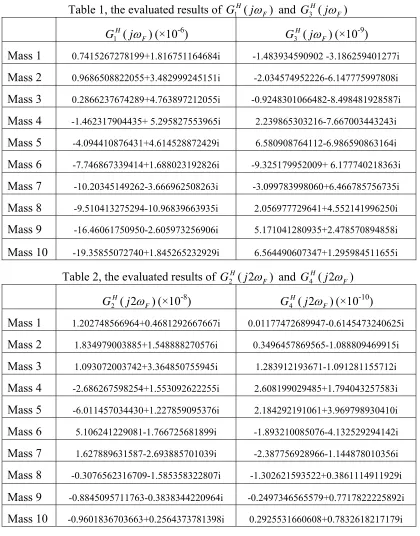
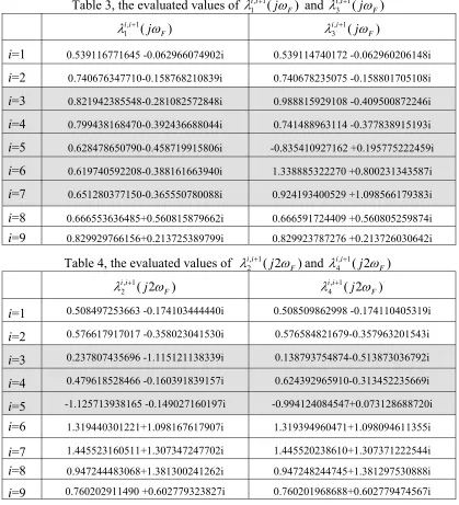
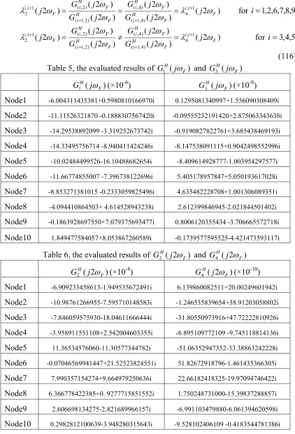
5 Numerical Study

To verify above analysis results, a damped 10-DOF oscillator was adopted, in which the fourth and sixth spring were nonlinear. The damping was assumed to be proportional damping, e.g., C=µK. The values of the system parameters are

1

10

1 = =m =