Table of Contents
Chapter 0: Front Matter ... 1
Dedication ... 1
Introduction ... 1
Who is this book for? ... 2
Chapter summaries ... 3
The project ... 4
Acknowledgements ... 5
Contact us ... 6
Chapter 1: Linking and Loading ... 7
What do linkers and loaders do? ... 7
Address binding: a historical perspective ... 7
Linking vs. loading ... 10
Tw o-pass linking ... 12
Object code libraries ... 15
Relocation and code modification ... 17
Compiler Drivers ... 18
Linker command languages ... 19
Linking: a true-life example ... 20
Exercises ... 25
Chapter 2: Architectural Issues ... 27
Application Binary Interfaces ... 27
Memory Addresses ... 28
Byte Order and Alignment ... 28
Address formation ... 30
Instruction formats ... 31
Procedure Calls and Addressability ... 32
Data and instruction references ... 36
IBM 370 ... 37
SPARC ... 40
SPARC V8 ... 40
SPARC V9 ... 42
Intel x86 ... 43
Paging and Virtual Memory ... 45
The program address space ... 48
Mapped files ... 49
Shared libraries and programs ... 51
Position-independent code ... 51
Intel 386 Segmentation ... 53
Embedded architectures ... 55
Address space quirks ... 56
Non-uniform memory ... 56
Memory alignment ... 57
Exercises ... 57
Chapter 3: Object Files ... 59
What goes into an object file? ... 59
Designing an object format ... 60
The null object format: MS-DOS .COM files ... 61
Code sections: Unix a.out files ... 61
a.out headers ... 64
Interactions with virtual memory ... 65
Relocation: MS-DOS EXE files ... 72
Symbols and relocation ... 74
Relocatable a.out ... 75
Relocation entries ... 78
Symbols and strings ... 80
a.out summary ... 82
Unix ELF ... 82
Relocatable files ... 85
ELF executable files ... 92
IBM 360 object format ... 94
ESD records ... 95
TXT records ... 97
RLD records ... 97
END records ... 98
Summary ... 98
Microsoft Portable Executable format ... 99
PE special sections ... 105
Running a PE executable ... 107
PE and COFF ... 107
PE summary ... 108
Intel/Microsoft OMF files ... 108
OMF records ... 110
Details of an OMF file ... 111
Summary of OMF ... 114
Comparison of object formats ... 114
Project ... 115
Exercises ... 117
Chapter 4: Storage allocation ... 119
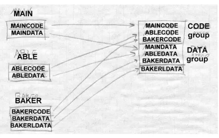
Segments and addresses ... 119
Simple storage layout ... 120
Multiple segment types ... 121
Segment and page alignment ... 124
Common blocks and other special segments ... 125
Common ... 125
C++ duplicate removal ... 127
Initializers and finalizers ... 130
IBM pseudo-registers ... 131
Special tables ... 134
X86 segmented storage allocation ... 134
Linker control scripts ... 136
Embedded system storage allocation ... 138
Storage allocation in practice ... 138
Storage allocation in ELF ... 141
Storage allocation in Windows linkers ... 144
Exercises ... 146
Project ... 147
Chapter 5: Symbol management ... 149
Binding and name resolution ... 149
Symbol table formats ... 150
Module tables ... 153
Global symbol table ... 154
Symbol resolution ... 157
Special symbols ... 158
Name mangling ... 158
Simple C and Fortran name mangling ... 158
C++ type encoding: types and scopes ... 160
Link-time type checking ... 163
Weak external and other kinds of symbols ... 164
Maintaining debugging information ... 164
Line number information ... 164
Symbol and variable information ... 165
Practical issues ... 166
Exercises ... 167
Project ... 167
Chapter 6: Libraries ... 169
Purpose of libraries ... 169
Library formats ... 169
Using the operating system ... 169
Unix and Windows Archive files ... 170
Unix archives ... 170
Extension to 64 bits ... 174
Intel OMF libraries ... 174
Creating libraries ... 176
Performance issues ... 179
Weak external symbols ... 179
Exercises ... 181
Project ... 181
Chapter 7: Relocation ... 183
Hardware and software relocation ... 183
Link time and load time relocation ... 184
Symbol and segment relocation ... 185
Symbol lookups ... 186
Basic relocation techniques ... 186
Instruction relocation ... 188
X86 instruction relocation ... 189
SPARC instruction relocation ... 189
ECOFF segment relocation ... 191
ELF relocation ... 193
OMF relocation ... 193
Relinkable and relocatable output formats ... 194
Other relocation formats ... 194
Chained references ... 195
Bit maps ... 195
Special segments ... 196
Relocation special cases ... 197
Exercises ... 197
Project ... 198
Chapter 8: Loading and overlays ... 201
Basic loading ... 201
Basic loading, with relocation ... 202
Position-independent code ... 203
TSS/360 position independent code ... 203
Per-routine pointer tables ... 206
Table of Contents ... 207
PIC costs and benefits ... 212
Bootstrap loading ... 213
Tree structured overlays ... 214
Defining overlays ... 217
Implementation of overlays ... 220
Overlay fine points ... 222
Data ... 222
Duplicated code ... 222
Multiple regions ... 223
Overlay summary ... 223
Exercises ... 223
Project ... 224
Chapter 9: Shared libraries ... 227
Binding time ... 230
Shared libraries in practice ... 231
Address space management ... 231
Structure of shared libraries ... 232
Creating shared libraries ... 233
Creating the jump table ... 234
Creating the shared library ... 235
Creating the stub library ... 235
Version naming ... 237
Linking with shared libraries ... 238
Running with shared libraries ... 238
The malloc hack, and other shared library problems ... 240
Exercises ... 243
Project ... 244
Chapter 10: Dynamic Linking and Loading ... 247
ELF dynamic linking ... 248
Contents of an ELF file ... 248
Loading a dynamically linked program ... 253
Finding the libraries ... 254
Shared library initialization ... 255
Lazy procedure linkage with the PLT ... 256
Other peculiarities of dynamic linking ... 258
Static initializations ... 258
Library versions ... 259
Dynamic loading at runtime ... 260
Microsoft Dynamic Link Libraries ... 260
Imported and exported symbols in PE files ... 261
Lazy binding ... 266
DLLs and threads ... 267
OSF/1 pseudo-static shared libraries ... 267
Making shared libraries fast ... 268
Comparison of dynamic linking approaches ... 270
Exercises ... 271
Project ... 271
Chapter 11: Advanced techniques ... 273
Techniques for C++ ... 273
Trial linking ... 274
Duplicate code elimination ... 276
Database approaches ... 278
Incremental linking and relinking ... 278
Link time garbage collection ... 281
Link time optimization ... 282
Link time code generation ... 284
Link-time profiling and instrumentation ... 284
Link time assembler ... 285
Load time code generation ... 285
The Java linking model ... 287
Loading Java classes ... 288
Exercises ... 290
Chapter 12: References ... 293
Chapter 0
Front Matter
$Revision: 2.2 $
$Date: 1999/06/09 00:48:48 $
Dedication
To Tonia and Sarah, my women folk.
Introduction
Linkers and loaders have been part of the software toolkit almost as long as there have been computers, since they are the critical tools that permit programs to be built from modules rather than as one big monolith.
As early as 1947, programmers started to use primitive loaders that could take program routines stored on separate tapes and combine and relocate them into one program. By the early 1960s, these loaders had evolved into full-fledged linkage editors. Since program memory remained expensive and limited and computers were (by modern standards) slow, these linkers contained complex features for creating complex memory overlay struc-tures to cram large programs into small memory, and for re-editing previ-ously linked programs to save the time needed to rebuild a program from scratch.
Who is this book for?
This book is intended for several overlapping audiences.
• Students: Courses in compiler construction and operating systems
have generally given scant treatment to linking and loading, often because the linking process seemed trivial or obvious. Although this was arguably true when the languages of interest were Fortran, Pascal, and C, and operating systems didn’t use memory mapping or shared libraries, it’s much less true now. C++, Java, and other object-oriented languages require a much more sophisticated link-ing environment. Memory mapped executable program, shared li-braries, and dynamic linking affect many parts of an operating sys-tem, and an operating system designer disregards linking issues at his or her peril.
• Practicing programmers also need to be aware of what linkers do,
again particularly for modern languages. C++ places unique de-mands on a linker, and large C++ programs are prone to develop hard-to-diagnose bugs due to unexpected things that happen at link time. (The best known are static constructors that run in an an or-der the programmer wasn’t expecting.) Linker features such as shared libraries and dynamic linking offer great flexibility and power, when used appropriately,
• Language designers and developers need to be aware of what
(The people who write linkers also all need this book, of course. But all the linker writers in the world could probably fit in one room and half of them already have copies because they reviewed the manuscript.)
Chapter summaries
Chapter 1, Linking and Loading, provides a short historical overview of the linking process, and discusses the stages of the linking process. It ends with a short but complete example of a linker run, from input object files to runnable ‘‘Hello, world’’ program.
Chapter 2, Architectural Issues, reviews of computer architecture from the point of view of linker design. It examines the SPARC, a representative reduced instruction set architecture, the IBM 360/370, an old but still very viable register-memory architecture. and the Intel x86, which is in a cate-gory of its own. Important architectural aspects include memory architec-ture, program addressing architecarchitec-ture, and the layout of address fields in individual instructions.
Chapter 3, Object Files, examines the internal structure of object and ex-ecutable files. It starts with the very simplest files, MS-DOS .COM files, and goes on to examine progressively more complex files including, DOS EXE, Windows COFF and PE (EXE and DLL), Unix a.out and ELF, and Intel/Microsoft OMF.
Chapter 4, Storage allocation, covers the first stage of linking, allocating storage to the segments of the linked program, with examples from real linkers.
Chapter 5, Symbol management, covers symbol binding and resolution, the process in which a symbolic reference in one file to a name in a second file is resolved to a machine address.
Chapter 6, Libraries, covers object code libraries, creation and use, with issues of library structure and performance.
so.
Chapter 8, Loading and overlays, covers the loading process, getting a program from a file into the computer’s memory to run. It also covers tree-structured overlays, a venerable but still effective technique to con-serve address space.
Chapter 9, Shared libraries, looks at what’s required to share a single copy of a library’s code among many different programs. This chapter concen-trates on static linked shared libraries.
Chapter 10, Dynamic Linking and Loading, continues the discussion of Chapter 9 to dynamically linked shared libraries. It treats two examples in detail, Windows32 dynamic link libraries (DLLs), and Unix/Linux ELF shared libraries.
Chapter 11, Advanced techniques, looks at a variety of things that sophisti-cated modern linkers do. It covers new features that C++ requires, includ-ing ‘‘name manglinclud-ing’’, global constructors and destructors, template ex-pansion, and duplicate code elimination. Other techniques include incre-mental linking, link-time garbage collection, link time code generation and optimization, load time code generation, and profiling and instrumenta-tion. It concludes with an overview of the Java linking model, which is considerably more semantically complex than any of the other linkers cov-ered.
Chapter 12, References, is an annotated bibliography.
The project
The initial project in Chapter 3 builds a linker skeleton that can read and write files in a simple but complete object format, and subsequent chapters add functions to the linker until the final result is a full-fledged linker that supports shared libraries and produces dynamically linkable objects.
Perl is quite able to handle arbitrary binary files and data structures, and the project linker could if desired be adapted to handle native object for-mats.
Acknowledgements
Many, many, people generously contributed their time to read and review the manuscript of this book, both the publisher’s reviewers and the readers of the comp.compilers usenet newsgroup who read and commented on an on-line version of the manuscript. They include, in alphabetical order, Mike Albaugh, Rod Bates, Gunnar Blomberg, Robert Bowdidge, Keith Breinholt, Brad Brisco, Andreas Buschmann, David S. Cargo, John Carr, David Chase, Ben Combee, Ralph Corderoy, Paul Curtis, Lars Duening, Phil Edwards, Oisin Feeley, Mary Fernandez, Michael Lee Finney, Peter H. Froehlich, Robert Goldberg, James Grosbach, Rohit Grover, Quinn Tyler Jackson, Colin Jensen, Glenn Kasten, Louis Krupp, Terry Lambert, Doug Landauer, Jim Larus, Len Lattanzi, Greg Lindahl, Peter Ludemann, Steven D. Majewski, John McEnerney, Larry Meadows, Jason Merrill, Carl Montgomery, Cyril Muerillon, Sameer Nanajkar, Jacob Navia, Simon Peyton-Jones, Allan Porterfield, Charles Randall, Thomas David Rivers, Ken Rose, Alex Rosenberg, Raymond Roth, Timur Safin, Kenneth G Salter, Donn Seeley, Aaron F. Stanton, Harlan Stenn, Mark Stone, Robert Strandh, Bjorn De Sutter, Ian Taylor, Michael Trofimov, Hans Walheim, and Roger Wong.
These people are responsible for most of the true statements in the book. The false ones remain the author’s responsiblity. (If you find any of the latter, please contact me at the address below so they can be fixed in subse-quent printings.)
Contact us
This book has a supporting web site at http://linker.iecc.com. It includes example chapters from the book, samples of perl code and ob-ject files for the proob-ject, and updates and errata.
Chapter 1
Linking and Loading
$Revision: 2.3 $
$Date: 1999/06/30 01:02:35 $
What do linkers and loaders do?
The basic job of any linker or loader is simple: it binds more abstract * names to more concrete names, which permits programmers to write code * using the more abstract names. That is, it takes a name written by a pro- * grammer such as getlineand binds it to ‘‘the location 612 bytes from * the beginning of the executable code in moduleiosys.’’ Or it may take a * more abstract numeric address such as ‘‘the location 450 bytes beyond the * beginning of the static data for this module’’ and bind it to a numeric ad- * dress. *
Address binding: a historical perspective
A useful way to get some insight into what linkers and loaders do is to look at their part in the development of computer programming systems.
The earliest computers were programmed entirely in machine language. Programmers would write out the symbolic programs on sheets of paper, hand assemble them into machine code and then toggle the machine code into the computer, or perhaps punch it on paper tape or cards. (Real hot-shots could compose code directly at the switches.) If the programmer used symbolic addresses at all, the symbols were bound to addresses as the programmer did his or her hand translation. If it turned out that an instruc-tion had to be added or deleted, the entire program had to be hand-inspect-ed and any addresses affecthand-inspect-ed by the addhand-inspect-ed or delethand-inspect-ed instruction adjusthand-inspect-ed.
Libraries of code compound the address assignment problem. Since the basic operations that computers can perform are so simple, useful pro-grams are composed of subpropro-grams that perform higher level and more complex operations. computer installations keep a library of pre-written and debugged subprograms that programmers can draw upon to use in new programs they write, rather than requiring programmers to write all their own subprograms. The programmer then loads the subprograms in with the main program to form a complete working program.
Programmers were using libraries of subprograms even before they used assemblers. By 1947, John Mauchly, who led the ENIAC project, wrote about loading programs along with subprograms selected from a catalog of programs stored on tapes, and of the need to relocate the subprograms’ code to reflect the addresses at which they were loaded. Perhaps surpris-ingly, these two basic linker functions, relocation and library search, ap-pear to predate even assemblers, as Mauchly expected both the program and subprograms to be written in machine language. The relocating loader allowed the authors and users of the subprograms to write each subpro-gram as though it would start at location zero, and to defer the actual ad-dress binding until the subprograms were linked with a particular main program.
As systems became more complex, they called upon linkers to do more and more complex name management and address binding. Fortran pro-grams used multiple subpropro-grams and common blocks, areas of data shared by multiple subprograms, and it was up to the linker to lay out stor-age and assign the addresses both for the subprograms and the common blocks. Linkers increasingly had to deal with object code libraries. in-cluding both application libraries written in Fortran and other languages, and compiler support libraries called implcitly from compiled code to han-dle I/O and other high-level operations.
Programs quickly became larger than available memory, so linkers provid-ed overlays, a technique that let programmers arrange for different parts of a program to share the same memory, with each overlay loaded on demand when another part of the program called into it. Overlays were widely used on mainframes from the advent of disks around 1960 until the spread of virtual memory in the mid-1970s, then reappeared on microcomputers in the early 1980s in exactly the same form, and faded as virtual memory appeared on PCs in the 1990s. They’re still used in memory limited em-bedded environments, and may yet reappear in other places where precise programmer or compiler control of memory usage improves performance.
binding any more than it already was, since addresses were still assigned at link time, but more work was deferred to the linker to assign addresses for all the sections.
Even when different programs are running on a computer, those different programs usually turn out to share a lot of common code. For example, nearly every program written in C uses routines such as fopen and
printf, database applications all use a large access library to connect to the database, and programs running under a GUI such as X Window, MS Windows, or the Macintosh all use pieces of the GUI library. Most sys-tems now provide shared libraries for programs to use, so that all the pro-grams that use a library can share a single copy of it. This both improves runtime performance and saves a lot of disk space; in small programs the common library routines often take up more space than the program itself.
In the simpler static shared libraries, each library is bound to specific ad-dresses at the time the library is built, and the linker binds program refer-ences to library routines to those specific addresses at link time. Static li-braries turn out to be inconveniently inflexible, since programs potentially have to be relinked every time any part of the library changes, and the de-tails of creating static shared libraries turn out to be very tedious. Systems added dynamically linked libraries in which library sections and symbols aren’t bound to actual addresses until the program that uses the library starts running. Sometimes the binding is delayed even farther than that; with full-fledged dynamic linking, the addresses of called procedures aren’t bound until the first call. Furthermore, programs can bind to li-braries as the programs are running, loading lili-braries in the middle of pro-gram execution. This provides a powerful and high-performance way to extend the function of programs. Microsoft Windows in particular makes extensive use of runtime loading of shared libraries (known as DLLs, Dy-namically Linked Libraries) to construct and extend programs.
Linking vs. loading
• Program loading: Copy a program from secondary storage (which
since about 1968 invariably means a disk) into main memory so it’s ready to run. In some cases loading just involves copying the data from disk to memory, in others it involves allocating storage, setting protection bits, or arranging for virtual memory to map vir-tual addresses to disk pages.
• Relocation: Compilers and assemblers generally create each file of
object code with the program addresses starting at zero, but few computers let you load your program at location zero. If a pro-gram is created from multiple subpropro-grams, all the subpropro-grams have to be loaded at non-overlapping addresses. Relocation is the process of assigning load addresses to the various parts of the pro-gram, adjusting the code and data in the program to reflect the as-signed addresses. In many systems, relocation happens more than once. It’s quite common for a linker to create a program from mul-tiple subprograms, and create one linked output program that starts at zero, with the various subprograms relocated to locations within the big program. Then when the program is loaded, the system picks the actual load address and the linked program is relocated as a whole to the load address.
• Symbol resolution: When a program is built from multiple
subpro-grams, the references from one subprogram to another are made using symbols; a main program might use a square root routine calledsqrt, and the math library definessqrt. A linker resolves the symbol by noting the location assigned to sqrt in the library, and patching the caller’s object code to so the call instruction refers to that location.
Although there’s considerable overlap between linking and loading, it’s reasonable to define a program that does program loading as a loader, and one that does symbol resolution as a linker. Either can do relocation, and there have been all-in-one linking loaders that do all three functions.
pro-gram, and treat relocatable addresses as references to the base address symbols.
One important feature that linkers and loaders share is that they both patch object code, the only widely used programs to do so other than perhaps de-buggers. This is a uniquely powerful feature, albeit one that is extremely machine specific in the details, and can lead to baffling bugs if done wrong.
Tw o-pass linking
Now we turn to the general structure of linkers. Linking, like compiling or assembling, is fundamentally a two pass process. A linker takes as its in-put a set of inin-put object files, libraries, and perhaps command files, and produces as its result an output object file, and perhaps ancillary informa-tion such as a load map or a file containing debugger symbols, Figure 1.
Figure 1-1: The linker process
When a linker runs, it first has to scan the input files to find the sizes of the segments and to collect the definitions and references of all of the symbols It creates a segment table listing all of the segments defined in the input files, and a symbol table with all of the symbols imported or exported.
Using the data from the first pass, the linker assigns numeric locations to symbols, determines the sizes and location of the segments in the output address space, and figures out where everything goes in the output file.
The second pass uses the information collected in the first pass to control the actual linking process. It reads and relocates the object code, substitut-ing numeric addresses for symbol references, and adjustsubstitut-ing memory ad-dresses in code and data to reflect relocated segment adad-dresses, and writes the relocated code to the output file. It then writes the output file, general-ly with header information, the relocated segments, and symbol table in-formation. If the program uses dynamic linking, the symbol table contains the info the runtime linker will need to resolve dynamic symbols. In many cases, the linker itself will generate small amounts of code or data in the output file, such as "glue code" used to call routines in overlays or dynam-ically linked libraries, or an array of pointers to initialization routines that need to be called at program startup time.
Whether or not the program uses dynamic linking, the file may also con-tain a symbol table for relinking or debugging that isn’t used by the pro-gram itself, but may be used by other propro-grams that deal with the output file.
Some object formats are relinkable, that is, the output file from one linker run can be used as the input to a subsequent linker run. This requires that the output file contain a symbol table like one in an input file, as well as all of the other auxiliary information present in an input file.
the debugger.
A few linkers appear to work in one pass. They do that by buffering some or all of the contents of the input file in memory or disk during the linking process, then reading the buffered material later. Since this is an imple-mentation trick that doesn’t fundamentally affect the two-pass nature of linking, we don’t address it further here.
Object code libraries
All linkers support object code libraries in one form or another, with most also providing support for various kinds of shared libraries.
The basic principle of object code libraries is simple enough, Figure 2. A library is little more than a set of object code files. (Indeed, on some sys-tems you can literally catenate a bunch of object files together and use the result as a link library.) After the linker processes all of the regular input files, if any imported names remain undefined, it runs through the library or libraries and links in any of the files in the library that export one or more undefined names.
Figure 1-2: Object code libraries
Relocation and code modification
The heart of a linker or loader’s actions is relocation and code modifica-tion. When a compiler or assembler generates and object file, it generates the code using the unrelocated addresses of code and data defined within the file, and usually zeros for code and data defined elsewhere. As part of the linking process, the linker modifies the object code to reflect the actual addresses assigned. For example, consider this snippet of x86 code that moves the contents of variableato variablebusing the eax register.
mov a,%eax mov %eax,b
Ifais defined in the same file at location 1234 hex and b is imported from somewhere else, the generated object code will be:
A1 34 12 00 00 mov a,%eax A3 00 00 00 00 mov %eax,b
Each instruction contains a one-byte operation code followed by a four-byte address. The first instruction has a reference to 1234 (four-byte reversed, since the x86 uses a right to left byte order) and the second a reference to zero since the location ofbis unknown.
Now assume that the linker links this code so that the section in whichais located is relocated by hex 10000 bytes, andbturns out to be at hex 9A12. The linker modifies the code to be:
A1 34 12 01 00 mov a,%eax A3 12 9A 00 00 mov %eax,b
That is, it adds 10000 to the address in the first instruction so now it refers to a’s relocated address which is 11234, and it patches in the address for
b. These adjustments affect instructions, but any pointers in the data part of an object file have to be adjusted as well.
compil-er and linkcompil-er have to use complicated addressing tricks to handle data at arbitrary addresses. In some cases, it’s possible to concoct an address us-ing two or three instructions, each of which contains part of the address, and use bit manipulation to combine the parts into a full address. In this case, the linker has to be prepared to modify each of the instructions ap-propriately, inserting some of the bits of the address into each instruction. In other cases, all of the addresses used by a routine or group of routines are placed in an array used as an ‘‘address pool’’, initialization code sets one of the machine registers to point to that array, and code loads pointers out of the address pool as needed using that register as a base register. The linker may have to create the array from all of the addresses used in a pro-gram, then modify instructions that so that they refer to the approprate ad-dress pool entry. We adad-dress this in Chapter 7.
Some systems require position independent code that will work correctly regardless of where in the address space it is loaded. Linkers generally have to provide extra tricks to support that, separating out the parts of the program that can’t be made position independent, and arranging for the two parts to communicate. (See Chapter 8.)
Compiler Drivers
In most cases, the operation of the linker is invisible to the programmer or nearly so, because it’s run automatically as part of the compilation pro-cess. Most compilation systems have a compiler driver that automatically invokes the phases of the compiler as needed. For example, if the pro-grammer has two C language source files, the compiler driver will run a sequence of programs like this on a Unix system:
• C preprocessor on file A, creating preprocessed A
• C compiler on preprocessed A, creating assembler file A
• Assembler on assembler file A, creating object file A
• C preprocceor on file B, creating preprocessed B
• Assembler on assembler file B, creating object file B
• Linker on object files A and B, and system C library
That is, it compiles each source file to assembler and then object code, and links the object code together, including any needed routines from the sys-tem C library.
Compiler drivers are often much cleverer than this. They often compare the creation dates of source and object files, and only recompile source files that have changed. (The Unix make program is the classic example.) Particularly when compiling C++ and other object oriented languages, compiler drivers can play all sorts of tricks to work around limitations in linkers or object formats. For example, C++ templates define a potentially infinite set of related routines, so to find the finite set of template routines that a program actually uses, a compiler driver can link the programs’ ob-ject files together with no template code, read the error messages from the linker to see what’s undefined, call the C++ compiler to generate object code for the necessary template routines and re-link. We cover some of these tricks in Chapter 11.
Linker command languages
Every linker has some sort of command language to control the linking process. At the very least the linker needs the list of object files and li-braries to link. Generally there is a long list of possible options: whether to keep debugging symbols, whether to use shared or unshared libraries, which of several possible output formats to use. Most linkers permit some way to specify the address at which the linked code is to be bound, which comes in handy when using a linker to link a system kernel or other pro-gram that doesn’t run under control of an operating system. In linkers that support multiple code and data segments, a linker command language can specify the order in which segments are to be linked, special treatment for certain kinds of segments, and other application-specific options.
There are four common techniques to pass commands to a linker:
• Command line: Most systems have a command line or the
sys-tems with limited length command lines, there’s usually a way to direct the linker to read commands from a file and treat them as though they were on the command line.
• Intermixed with object files: Some linkers, such as IBM mainframe
linkers, accept alternating object files and linker commands in a single input file. This dates from the era of card decks, when one would pile up object decks and hand-punched command cards in a card reader.
• Embedded in object files: Some object formats, notably
Mi-crosoft’s, permit linker commands to be embedded inside object files. This permits a compiler to pass any options needed to link an object file in the file itself. For example, the C compiler passes commands to search the standard C library.
• Separate configuration language: A few linkers have a full fledged
configuration language to control linking. The GNU linker, which can handle an enormous range of object file formats, machine ar-chitectures, and address space conventions, has a complex control language that lets a programmer specify the order in which ments should be linked, rules for combining similar segments, seg-ment addresses, and a wide range of other options. Other linkers have less complex languages to handle specific features such as programmer-defined overlays.
Linking: a true-life example
We complete our introduction to linking with a small but real linking ex-ample. Figure 3 shows a pair of C language source files, m.c with a main program that calls a routine named a, and a.c that contains the routine with a call to the library routinesstrlenandprintf.
Figure 1-3: Source files
Source file m.c
int main(int ac, char **av) {
static char string[] = "Hello, world!\n";
a(string); }
Source file a.c
#include <unistd.h> #include <string.h>
void a(char *s) {
write(1, s, strlen(s)); }
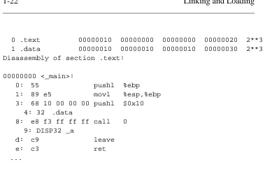
The main program m.c compiles, on my Pentium with GCC, into a 165 byte object file in the classic a.out object format, Figure 4. That object file includes a fixed length header, 16 bytes of "text" segment, containing the read only program code, and 16 bytes of "data" segment, containing the string. Following that are two relocation entries, one that marks the pushl instruction that puts the address of the string on the stack in preparation for the call toa, and one that marks the call instruction that transfers con-trol toa. The symbol table exports the definition of_main, imports _a, and contains a couple of other symbols for the debugger. (Each global symbol is prefixed with an underscore, for reasons described in Chapter 5.) Note that the pushl instruction refers to location 10 hex, the tentative address for the string, since it’s in the same object file, while the call refers to location 0 since the address of_ais unknown.
Figure 1-4: Object code for m.o
Sections:
0 .text 00000010 00000000 00000000 00000020 2**3 1 .data 00000010 00000010 00000010 00000030 2**3 Disassembly of section .text:
00000000 <_main>:
0: 55 pushl %ebp
1: 89 e5 movl %esp,%ebp 3: 68 10 00 00 00 pushl $0x10
4: 32 .data
8: e8 f3 ff ff ff call 0 9: DISP32 _a
d: c9 leave
e: c3 ret
...
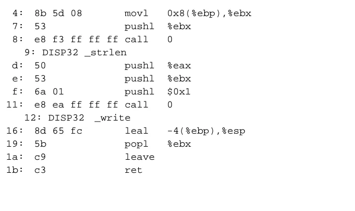
The subprogram file a.c compiles into a 160 byte object file, Figure 5, with the header, a 28 byte text segment, and no data. Tw o relocation entries mark the calls to strlen and write, and the symbol table exports _a
[image:31.595.140.519.147.412.2]and imports_strlenand_write.
Figure 1-5: Object code for m.o
Sections:
Idx Name Size VMA LMA File off Algn
0 .text 0000001c 00000000 00000000 00000020 2**2 CONTENTS, ALLOC, LOAD, RELOC, CODE
1 .data 00000000 0000001c 0000001c 0000003c 2**2 CONTENTS, ALLOC, LOAD, DATA
Disassembly of section .text:
00000000 <_a>:
0: 55 pushl %ebp
1: 89 e5 movl %esp,%ebp
4: 8b 5d 08 movl 0x8(%ebp),%ebx
7: 53 pushl %ebx
8: e8 f3 ff ff ff call 0 9: DISP32 _strlen
d: 50 pushl %eax
e: 53 pushl %ebx
f: 6a 01 pushl $0x1 11: e8 ea ff ff ff call 0
12: DISP32 _write
16: 8d 65 fc leal -4(%ebp),%esp
19: 5b popl %ebx
1a: c9 leave
1b: c3 ret
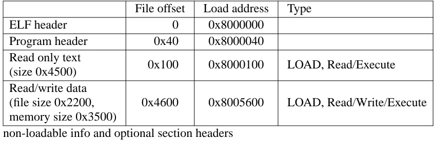
[image:32.595.150.503.191.401.2]To produce an executable program, the linker combines these two object files with a standard startup initialization routine for C programs, and nec-essary routines from the C library, producing an executable file displayed in part in Figure 6.
Figure 1-6: Selected parts of executable
Sections:
Idx Name Size VMA LMA File off Algn
0 .text 00000fe0 00001020 00001020 00000020 2**3 1 .data 00001000 00002000 00002000 00001000 2**3 2 .bss 00000000 00003000 00003000 00000000 2**3
Disassembly of section .text:
00001020 <start-c>: ...
1092: e8 0d 00 00 00 call 10a4 <_main> ...
10a4: 55 pushl %ebp 10a5: 89 e5 movl %esp,%ebp 10a7: 68 24 20 00 00 pushl $0x2024 10ac: e8 03 00 00 00 call 10b4 <_a>
10b1: c9 leave
10b2: c3 ret
...
000010b4 <_a>:
10b4: 55 pushl %ebp
10b5: 89 e5 movl %esp,%ebp
10b7: 53 pushl %ebx
10b8: 8b 5d 08 movl 0x8(%ebp),%ebx
10bb: 53 pushl %ebx
10bc: e8 37 00 00 00 call 10f8 <_strlen>
10c1: 50 pushl %eax
10c2: 53 pushl %ebx
10c3: 6a 01 pushl $0x1
10c5: e8 a2 00 00 00 call 116c <_write> 10ca: 8d 65 fc leal -4(%ebp),%esp
10cd: 5b popl %ebx
10ce: c9 leave
10cf: c3 ret
...
000010f8 <_strlen>: ...
0000116c <_write>: ...
The combined text segment contains the text of library startup code called
start-c, then text from m.o relocated to 10a4, a.o relocated to 10b4, and routines linked from the C library, relocated to higher addresses in the text segment. The data segment, not displayed here, contains the com-bined data segments in the same order as the text segments. Since the code for _main has been relocated to address 10a4 hex, that address is patched into the call instruction in start-c. Within the main routine, the reference to the string is relocated to 2024 hex, the string’s final location in the data segment, and the call is patched to 10b4, the final address of _a. Within_a, the calls to_strlenand_writeare patched to the final ad-dresses for those two routines.
The executable also contains about a dozen other routines from the C li-brary, not displayed here, that are called directly or indirectly from the startup code or from _write (error routines, in the latter case.) The ex-ecutable contains no relocation data, since this file format is not relinkable and the operating system loads it at a known fixed address. It contains a symbol table for the benefit of a debugger, although the executable doesn’t use the symbols and the symbol table can be stripped off to sav e space.
In this example, the code linked from the library is considerably larger than the code for the program itself. That’s quite common, particularly when programs use large graphics or windowing libraries, which provided the impetus for shared libraries, Chapters 9 and 10. The linked program is 8K, but the identical program linked using shared libraries is only 264 bytes. This is a toy example, of course, but real programs often have equally dramatic space savings.
Exercises
What is the advantage of separating a linker and loader into separate pro-grams? Under what circumstances would a combined linking loader be useful?
Nearly every programming system produced in the past 50 years includes a linker. Why?
Chapter 2
Architectural Issues
$Revision: 2.3 $
$Date: 1999/06/15 03:30:36 $
Linkers and loaders, along with compilers and assemblers, are exquisitely * sensitive to the architectural details, both the hardware architecture and the * architecture conventions required by the operating system of their target * computers. In this chapter we cover enough computer architecture to un- * derstand the jobs that linkers have to do. The descriptions of all of the * computer architectures in this chapter are deliberately incomplete and * leave out the parts that don’t affect the linker such as floating point and * I/O. *
Tw o aspects of hardware architecture affect linkers: program addressing * and instruction formats. One of the things that a linker does is to modify * addresses and offsets both in data memory and in instructions. In both * cases, the linker has to ensure that its modifications match the addressing * scheme that the computer uses; when modifying instructions it must fur- * ther ensure that the modifications don’t result in an invalid instruction. *
At the end of the chapter, we also look at address space architecture, that is, what set of addresses a program has to work with.
Application Binary Interfaces
Every operating system presents an Application Binary Interface (ABI) to programs that run under that system. The ABI consists of programming conventions that applications have to follow to run under the operating system. ABI’s inv ariably include a set of system calls and the technique to invoke the system calls, as well as rules about what memory addresses a program can use and often rules about usage of machine registers. From the point of view of an application, the ABI is as much a part of the system architecture as the underlying hardware architecture, since a program will fail equally badly if it violates the constraints of either.
program contains a table of all of the addresses of static data used by rou-tines in the program, the linker often creates that table, by collecting ad-dress information from all of the modules linked into the program. The aspect of the ABI that most often affects the linker is the definition of a standard procedure call, a topic we return to later in this chapter.
Memory Addresses
Every computer includes a main memory. The main memory invariably appears as an array of storage locations, with each location having a nu-meric address. The addresses start at zero and run up to some large num-ber determined by the numnum-ber of bits in an address.
Byte Order and Alignment
Each storage location consists of a fixed number of bits. Over the past 50 years computers have been designed with storage locations consisting of as many as 64 bits and as few as 1 bit, but now nearly every computer in production addresses 8 bit bytes. Since much of the data that computers handle, notably program addresses, are bigger than 8 bits, the computers can also handle 16, 32, and often 64 or 128 bit data as well, with multiple adjacent bytes grouped together. On some computers, notably those from IBM and Motorola, the first (numerically lowest addressed) byte in multi-byte data is the most significant multi-byte, while others, notably DEC and Intel, it’s the least significant byte, Figure 1. In a nod to Gulliver’s Travels the IBM/Motorola byte order scheme is known as big-endian while the DEC/Intel scheme is little-endian.
Figure 2-1: Byte addressable memory
The relative merits of the two schemes have provoked vehement argu-ments over the years. In practice the major issue determining the choice of byte order is compatibility with older systems, since it is considerably easier to port programs and data between two machines with the same byte order than between machines with different byte orders. Many recent chip designs can support either byte order, with the choice made either by the way the chip is wired up, by programming at system boot time, or in a few cases even selected per application. (On these switch-hitting chips, the byte order of data handled by load and store instructions changes, but the byte order of constants encoded in instructions doesn’t. This is the sort of detail that keeps the life of the linker writer interesting.)
work at the cost of reduced performance, while on others (most RISC chips), misaligned data causes a program fault. Even on systems where misaligned data don’t cause a fault, the performance loss is usually great enough that it’s worth the effort to maintain alignment where possible.
Many processors also have alignment requirements for program instruc-tions. Most RISC chips require that instructions be aligned on four-byte boundaries.
Each architecture also defines registers, a small set of fixed length high-speed memory locations to which program instructions can refer directly. The number of registers varies from one architecture to another, from as few as eight in the Intel architecture to 32 in some RISC designs. Regis-ters are almost invariably the same size as a program address, that is, on a system with 32 bit addresses, the registers are 32 bits, and on systems with 64 bit addresses, the registers are 64 bits as well.
Address formation
As a computer program executes, it loads and stores data to and from memory, as determined by instructions in the program. The instructions are themselves stored in memory, usually a different part of memory from the program’s data. Instructions are logically executed in the sequence they are stored, except that jump instructions specify a new place in the program to start executing instructions. (Some architectures use the term branch for some or all jumps, but we call them all jumps here.) Each in-struction that references data memory and each jump specifies the address or addresses or the data to load or store, or of the instruction to jump to. All computers have a variety of instruction formats and address formation rules that linkers have to be able to handle as they relocate addresses in in-structions.
• The IBM 360/370/390 (which we’ll refer to as the 370). Although this is one of the oldest architectures still in use, its relatively clean design has worn well despite 35 years of added features, and has been implemented in chips comparable in performance to modern RISCs.
• SPARC V8 and V9. A popular RISC architecture, with fairly sim-ple addressing. V8 uses 32 bit registers and addresses, V9 adds 64 bit registers and addresses. The SPARC design is similar to other RISC architectures such as MIPS and Alpha.
• The Intel 386/486/Pentium (henceforth x86). One of the most ar-cane and irregular architectures still in use, but undeniably the most popular.
Instruction formats
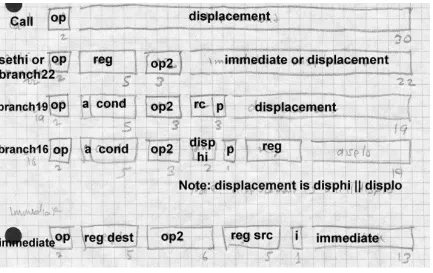
Each architecture has several different instruction formats. We’ll only ad-dress the format details relative to program and data adad-dressing, since those are the main details that affect the linker. The 370 uses the same for-mat for data references and jumps, while the SPARC has different forfor-mats and the x86 has some common formats and some different.
two are treated the same.
Other more complicated address calculation schemes are still in use, but for the most part the linker doesn’t hav e to worry about them since they don’t contain any fields the linker has to adjust.
Some architectures use fixed length instructions, and some use variable length instructions. All SPARC instructions are four bytes long, aligned on four byte boundaries. IBM 370 instructions can be 2, 4, or 6 bytes long, with the first two bits of the first byte determining the length and for-mat of the instruction. Intel x86 instructions can be anywhere from one byte to 14 long. The encoding is quite complex, partly because the x86 was originally designed for limited memory environments with a dense in-struction encoding, and partly because the new inin-structions added in the 286, 386, and later chips had to be shoe-horned into unused bit patterns in the existing instruction set. Fortunately, from the point of view of a linker writer, the address and offset fields that a linker has to adjust all occur on byte boundaries, so the linker generally need not be concerned with the in-struction encoding.
Procedure Calls and Addressability
In the earliest computers, memories were small, and each instruction con-tained an address field large enough to contain the address of any memory location in the computer, a scheme now called direct addressing. By the early 1960s, addressable memory was getting large enough that an tion set with a full address in each instruction would have large instruc-tions that took up too much of still-precious memory. To solve this prob-lem, computer architects abandoned direct addressing in some or all of the memory reference instructions, using index and base registers to provide most or all of the bits used in addressing. This allowed instructions to be shorter, at the cost of more complicated programming.
The bootstrap problem is to get the first base value into a register at the be-ginning of the program, and subsequently to ensure that each routine has the base values it needs to address the data it uses.
Procedure calls
Every ABI defines a standard procedure call sequence, using a combina-tion of hardware-defined call instruccombina-tions and convencombina-tions about register and memory use. A hardware call instruction saves the return address (the address of the instruction after the call) and jumps to the procedure. On architectures with a hardware stack such as the x86 the return address is pushed on the stack, while on other architectures it’s sav ed in a register, with software having the responsibility to save the register in memory if necessary. Architectures with a stack generally have a hardware return in-struction that pops the return address from the stack and jumps to that ad-dress, while other architectures use a ‘‘branch to address in register’’ in-struction to return.
Within a procedure, data addressing falls into four categories:
• The caller can pass arguments to the procedure.
• Local variables are allocated withing procedure and freed before
the procedure returns.
• Local static data is stored in a fixed location in memory and is
pri-vate to the procedure.
• Global static data is stored in a fixed location in memory and can
be referenced from many different procedures.
The chunk of stack memory allocated for a single procedure call is known as a stack frame. Figure 2 shows a typical stack frame.
Figure 2-2: Stack frame memory layout
frame pointer or base pointer register is loaded from the stack pointer at the time a procedure starts. This makes it possible to push variable sized objects on the stack, changing the value in the stack pointer register to a hard-to-predict value, but still lets the procedure address arguments and lo-cals at fixed offsets from the frame pointer which doesn’t change during a procedure’s execution. Assuming the stack grows from higher to lower addresses and that the frame pointer points to the address in memory where the return address is stored, arguments are at small positive offsets from the frame pointer, and local variables at negative offsets. The operat-ing system usually sets the initial stack pointer register before a program starts, so the program need only update the register as needed when it pushes and pops data.
For local and global static data, a compiler can generate a table of pointers to all of the static objects that a routine references. If one of the registers contains a pointer to this table, the routine can address any desired static object by loading the pointer to the object from the table using the table pointer register into another register using the table pointer register as a base register, then using that second register as the base register to address the object. The trick, then, is to get the address of the table into the first register. On SPARC, the routine can load the table address into the regis-ter using a sequence of instructions with immediate operands, and on the SPARC or 370 the routine can use a variant of a subroutine call instruction to load the program counter (the register that keeps the address of the cur-rent instruction) into a base register, though for reasons we discuss later, those techniques cause problems in library code. A better solution is to foist off the job of loading the table pointer on the routine’s caller, since the caller will have its own table pointer already loaded and can get ad-dress of the called routine’s table from its own table.
Figure 2-3: Idealized calling sequence
... push arguments on the stack ...
store Rt → xxx(Rf) ; save caller’s table pointer in caller’s stack frame load Rx ← MMM(Rt) ; load address of called routine into temp register load Rt ← NNN(Rt) ; load called routine’s table pointer
call (Rx) ; call routine at address in Rx
load Rt ← xxx(Rf) ; restore caller’s table pointer
Several optimizations are often possible. In many cases, all of the routines in a module share a single pointer table, in which case intra-module calls needn’t change the table pointer. The SPARC convention is that an entire library shares a single table, created by the linker, so the table pointer reg-ister can remain unchanged in intra-module calls. Calls within the same module can usually be made using a version of the ‘‘call’’ instruction with the offset to the called routine encoded in the instruction, which avoids the need to load the address of the routine into a register. With both of these optimizations, the calling sequence to a routine in the same module re-duces to a single call instruction.
To return to the address bootstram quesion, how does this chain of table pointers gets started? If each routine gets its table pointer loaded by the preceding routine, where does the initial routine get its pointer? The an-swer varies, but always involves special-case code. The main routine’s table may be stored at a fixed address, or the initial pointer value may be tagged in the executable file so the operating system can load it before the program starts. No matter what the technique is, it invariably needs some help from the linker.
Data and instruction references
IBM 370
The 1960s vintage System/360 started with a very straightforward data ad-dressing scheme, which has become someone more complicated over the years as the 360 evolved into the 370 and 390. Every instruction that ref-erences data memory calculates the address by adding a 12-bit unsigned offset in the instruction to a base register and maybe an index register. There are 16 general registers, each 32 bits, numbered from 0 to 15, all but one of which can be used as index registers. If register 0 is specified in an address calculation, the value 0 is used rather than the register contents. (Register 0 exists and is usable for arithmetic, but not for addressing.) In instructions that take the target address of a jump from a register, register 0 means don’t jump.
Figure 4 shows the major instruction formats. An RX instruction contains a register operand and a single memory operand, whose address is calcu-lated by adding the offset in the instruction to a base register and index register. More often than not the index register is zero so the address is just base plus offset. In the RS, SI and SS formats, the 12 bit offset is added to a base register. An RS instruction has one memory operand, with one or two other operands being in registers. An SI instruction has one memory operand, the other operand being an immediate 8 bit value in the instruction An SS instruciton has two memory operands, storage to storage operations. The RR format has two register operands and no memory operands at all, although some RR instructions interpret one or both of the registers as pointers to memory. The 370 and 390 added some minor vari-ations on these formats, but none with different data addressing formats.
Figure 2-4: IBM 370 instruction formats
Instructions can directly address the lowest 4096 locations in memory by specifying base register zero. This ability is essential in low-level system programming but is never used in application programs, all of which use base register addressing.
Note that in all three instruction formats, the 12 bit address offset is al-ways stored as the low 12 bits of a 16-bit aligned halfword. This makes it possible to specify fixups to address offsets in object files without any ref-erence to instruction formats, since the offset format is always the same.
31 bit addresses. A convention enforced by a combination of hardware and software states that an address word with the high bit set contains a 31 bit address in the rest of the word, while one with the high bit clear con-tains a 24 bit address. As a result, a linker has to be able to handle both 24 bit and 31 bit addresses since programs can and do switch modes depend-ing on how long ago a particular routine was written. For historical rea-sons, 370 linkers also handle 16 bit addresses, since early small models in the 360 line often had 64K or less of main memory and programs used load and store halfword instructions to manipulate address values.
Later models of the 370 and 390 added segmented address spaces some-what like those of the x86 series. These feature let the operating system define multiple 31 bit address spaces that a program can address, with ex-tremely complex rules defining access controls and address space switch-ing. As far as I can tell, there is no compiler or linker support for these features, which are primarily used by high-performace database systems, so we won’t address them further.
Instruction addressing on the 370 is also relatively straightforward. In the original 360, the jumps (always referred to as branch instructions) were all RR or RX format. In RR jumps, the second register operand contained the jump target, register 0 meaning don’t jump. In RX jumps, the memory operand is the jump target. The procedure call is Branch and Link (sup-planted by the later Branch and Store for 31 bit addressing), which stores the return address in a specified register and then jumps to the address in the second register in the RR form or to the second operand address in the RX form.
registers to cover all of the routine’s code.
The 390 added relative forms of all of the jumps. In these new forms, the instruction contains a signed 16 bit offset which is logically shifted left one bit (since instructions are aligned on even bytes) and added to the ad-dress of the instruction to get the adad-dress of the jump target. These new formats use no register to compute the address, and permit jumps within +/- 64K bytes, enough for intra-routine jumps in all but the largest rou-tines.
SPARC
The SPARC comes close to living up to its name as a reduced instruction set processor, although as the architecture has evolved through nine ver-sions, the original simple design has grown somewhat more complex. SPARC versions through V8 are 32 bit architectures. SPARC V9 expands the architecture to 64 bits.
SPARC V8
SPARC has four major instruction formats and 31 minor instruction for-mats, Figure 5, four jump forfor-mats, and two data addressing modes.
In SPARC V8, there are 31 general purpose registers, each 32 bits, num-bered from 1 to 31. Register 0 is a pseudo-register that always contains the value zero.
An unusual register window scheme attempts to minimize the amount of register saving and restoring at procedure calls and returns. The windows have little effect on linkers, so we won’t discuss them further. (Register windows originated in the Berkeley RISC design from which SPARC is descended.)
SPARC assemblers and linkers support a pseudo-direct addressing scheme using a two-instruction sequence. The two instructions are SETHI, which loads its 22 bit immediate value into the high 22 bits of a register and ze-ros the lower 10 bits, followed by OR Immediate, which ORs its 13 bit im-mediate value into the low part of the register. The assembler and linker arrange to put the high and low parts of the desired 32 bit address into the two instructions.
Figure 2-5: SPARC
30 bit call 22 bit branch and SETHI 19 bit branch 16 bit branch (V9 only) op R+R op R+I13
various size branch offsets ranging from 16 to 30 bits. Whatever the offset size, the jump shifts the offset two bits left, since all instructions have to be at four-byte word addresses, sign extends the result to 32 or 64 bits, and adds that value to the address of the jump or call instruction to get the tar-get address. The call instruction uses a 30 bit offset, which means it can reach any address in a 32 bit V8 address space. Calls store the return ad-dress in register 15. Various kinds of jumps use a 16, 19, or 22 bit offset, which is large enough to jump anywhere in any plausibly sized routine. The 16 bit format breaks the offset into a two-bit high part and a fourteen-bit low part stored in different parts of the instruction word, but that doesn’t cause any great trouble for the linker.
SPARC also has a "Jump and Link" which computes the target address the same way that data reference instructions do, by adding together either two source registers or a source register and a constant offset. It also can store the the return address in a target register.
Procedure calls use Call or Jump and Link, which store the return address in register 15, and jumps to the target address. Procedure return uses JMP 8[r15], to return two instructions after the call. (SPARC calls and jumps are "delayed" and optionally execute the instruction following the jump or call before jumping.)
SPARC V9
Intel x86
The Intel x86 architecture is by far the most complex of the three that we discuss. It features an asymmetrical instruction set and segmented ad-dresses. There are six 32 bit general purpose registers named EAX, EBX, ECX, EDX, ESI, and EDI, as well as two registers used primarily for ad-dressing, EBP and ESP, and six specialized 16 bit segment registers CS, DS, ES, FS, GS, and SS. The low half of each of the 32 bit registers can be used as 16 bit registers called AX, BX, CX, DX, SI, DI, BP, and SP. and the low and high bytes of each of the AX through DX registers are eight-bit registers called AL, AH, BL, BH, CL, CH, DL, and DH. On the 8086, 186, and 286, many instructions required its operands in specific registers, but on the 386 and later chips, most but not all of the functions that required specific registers have been generalized to use any register. The ESP is the hardware stack pointer, and always contains the address of the current stack. The EBP pointer is usually used as a frame register that points to the base of the current stack frame. (The instruction set encour-ages but doesn’t require this.)
At any moment an x86 is running in one of three modes: real mode which emulates the original 16 bit 8086, 16 bit protected mode which was added on the 286, or 32 bit protected mode which was added on the 386. Here we primarily discuss 32 bit protected mode. Protected mode involves the x86’s notorious segmentation, but we’ll disregard that for the moment.
Most instructions that address addresses of data in memory use a common instruction format, Figure 6. (The ones that don’t use specific architecture defined registers, e.g., the PUSH and POP instructions always use ESP to address the stack.) Addresses are calculated by adding together any or all of a signed 1, 2, or 4 byte displacement value in the instruction, a base reg-ister which can be any of the 32 bit regreg-isters, and an optional index regis-ter which can be any of the 32 bit regisregis-ters except ESP. The index can be logically shifted left 0, 1, 2, or 3 bits to make it easier to index arrays of multi-byte values.
one or two opcode bytes, optional mod R/M byte, optional s-i-b byte, optional 1, 2, or 4 byte displacement
Although it’s possible for a single instruction to include all of displace-ment, base, and index, most just use a 32 bit displacedisplace-ment, which provides direct addressing, or a base with a one or two byte displacement, which provides stack addressing and pointer dereferencing. From a linker’s point of view, direct addressing permits an instruction or data address to be em-bedded anywhere in the program on any byte boundary.
described above, most often used to jump or call to an address stored in a register. Call instructions push the return address on the stack pointed to by ESP.
Unconditional jumps and calls can also have a full six byte segment/offset address in the instruction, or calculate the address at which the seg-ment/offset target address is stored. These call instructions push both the return address and the caller’s segment number, to permit intersegment calls and returns.
Paging and Virtual Memory
On most modern computers, each program can potentially address a vast amount of memory, four gigabytes on a typical 32 bit machine. Few com-puters actually have that much memory, and even the ones that do need to share it among multiple programs. Paging hardware divides a program’s address space into fixed size pages, typically 2K or 4K bytes in size, and divides the physical memory of the computer into page frames of the same size. The hardware conatins page tables with an entry for each page in the address space, as shown in Figure 7.
Figure 2-7: Page mapping
a copy of the contents page from disk into a free page frame, then let the application continue. By moving pages back and forth between main memory and disk as needed, the operating system can provide virtual
memory which appears to the application to be far larger than the real
memory in use.
Virtual memory comes at a cost, though. Individual instructions execute in a fraction of a microsecond, but a page fault and consequent page in or page out (transfer from disk to main memory or vice versa) takes several milliseconds since it requires a disk transfer. The more page faults a pro-gram generates, the slower it runs, with the worst case being thrashing, all page faults with no useful work getting done. The fewer pages a program needs, the fewer page faults it will generate. If the linker can pack related routines into a single page or a small group of pages, paging performance improves.
If pages can be marked as read-only, performace also improves. Read-on-ly pages don’t need to be paged out since they can be reloaded from wher-ev er they came from originally. If identical pages logically appear in mul-tiple address spaces, which often happens when mulmul-tiple copies of the same program are running, a single physical page suffices for all of the ad-dress spaces.
contains 1024 entries. Each lower level page table also contains 1024 en-tries to map the 1024 4K pages in the 4MB of address space correspond-ing to that page table. The SPARC architecture defines the page size as 4K, and has three levels of page tables rather than two.
The two- or three-level nature of page tables are invisible to applications with one important exception: the operating system can change the map-ping for a large chunk of the address space (1MB on the 370, 4MB on the x86, 256K or 16MB on SPARC) by changing a single entry in an upper level page table, so for efficiency reasons the address space is often man-aged in chunks of that size by replacing individual second level page table entries rather than reloading the whole page table on process switches.
The program address space
Every application program runs in an address space defined by a combina-tion of the computer’s hardware and operating system. The linker or load-er needs to create a runnable program that matches that address space.
The simplest kind of address space is that provided by PDP-11 versions of Unix. The address space is 64K bytes starting at location zero. The read-only code of the program is loaded at location zero, with the read-write da-ta following the code. The PDP-11 had 8K pages, so the dada-ta sda-tarts on the 8K boundary after the code. The stack grows downward, starting at 64K-1, and as the stack and data grow, the respective areas were enlarged; if they met the program ran out of space. Unix on the VAX, the follow-on to the PDP-11, used a similar scheme. The first two bytes of every VAX Unix program were zero (a register save mask saying not to save any-thing.) As a result, a null all-zero pointer was always valid, and if a C pro-gram used a null value as a string pointer, the zero byte at location zero was treated as a null string. As a result, a generation of Unix programs in the 1980s contained hard-to-find bugs involving null pointers, and for many years, Unix ports to other architectures provided a zero byte at loca-tion zero because it was easier than finding and fixing all the null pointer bugs.