C
OMPUTATIONAL
A
NALYSIS OF
D
YNAMICS WITHIN THE
NUCLEAR FACTOR-KAPPAB SIGNALLING SYSTEM
Thesis submitted in accordance with the requirements of the University of Liverpool
for the degree of Doctor in Philosophy
by
Declaration
!
!
!
!
!
"!i!"!
Declaration
This thesis is the result of my own work, unless otherwise stated, and it is based upon
the results from experimental and theoretical work performed as a PhD student
between October 2009 and July 2012 in the department of Biological Sciences within
the University of Liverpool.
Neither this thesis nor any part of it has been submitted in support of an application
for another degree or qualification at this or any other University or other institute of
learning.
Acknowledgements
!
!
!
!
"!ii!"!
Acknowledgements
There are many people who have aided me in the completion of this task - a big thank you to all of you. Firstly, I’d like to thank my supervisors Prof Chris Sanderson, Dr Rachel Bearon and Prof Mike White. Thanks for all the support and opportunities you have given me, and everything you have done to help me to complete this thesis on an accelerated schedule.
In addition to my supervisors there are many people that I have worked with and without their advice and encouragement I would not have reached this point. A very BIG thanks to Pawel Paszek, while his criticism has been plentiful it is always constructive and without his guidance over the last three years I would not have completed my PhD. Thanks must also go to Prof Vadim Biktashev who helped to make a reluctant student more rigorous and has put me on the path to my first publication. Thanks to Dan Woodcock (aka #2) for all his help and suggestions when the NF-κB world was getting a little hotter. Thanks to Cath Heyward my diclofenac buddy and neighbour, who in addition to dealing with my many questions over the last year also proof read this tome – yes typos are her fault! Many thanks to Dave Spiller for his A20 suggestions, mad microscope skills and the occasional pint! I would also like to thank John ‘the Daddy’ Ankers, James ‘the actual daddy’ Bagnall and Damon Daniels for all their advice and generally listening to my complaining. There are many other people both in Liverpool and Manchester who have helped over the years. Dr Violaine See for giving me a home for the last 18 months. Many thanks to Anne H, Haleh, Carol and Sarah for the delicious cake and the gossip. Thank you to Anne M, Anthony, Claire, Connie, David T, Louise, Nisha, Sheila, Steph, and Raheela for you lab help, friendship and advice over the last three years. To everybody else who has been a part of the See and White groups thank you very, very much, unfortunately I can’t list you all as I’m trying to keep this to a page. Finally a big heads up to my fellow SABR students Karen and James who have been with me from the beginning. It has been a memorable four years and that is thanks to you guys and your unconventional attitude towards life!
Beyond work thanks to everyone who has been a fried over the years. The PhD students at Liverpool who I’ve enjoyed lunching with over the last three years, those include Jane, Louise, Jen, Jo and many more. Thanks to my housemates Jenna, Tash and Indy. The ‘House of Hot’ has been an epic place to live and I will miss you lots. All the tramps for giving such good banter over the years and keeping me young in spirit if not in body! Everyone who was part of the MSc at Warwick especially Jo, Joe and Mrs Lewis. Dominic Francis Graham Holdaway for the red wine, Mario Kart and TV cookery backup plan. My Bath buddies Gen, James, Jess, Jo, Laura, Rees and Tam. Many thanks to Sean for everything, but mainly dealing with a moodier Simon than everyone else! Finally thank you to Mum, Dad, Phil, Teresa, Nina, Jay and the Grandparents for all your help and support both financial and emotional over the last 25 years, and for not saying too much when I told you I was going to do another 4 year study!
Abstract
!
!
!
!
"!iii!"!
Abstract
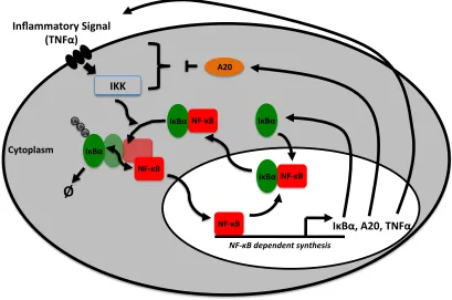
The Nuclear Factor kappaB (NF-κB) proteins are a very important family of transcription factors. The signalling system of the NF-κB transcription factors drives cellular inflammation and immune responses, playing a central role in cell proliferation and apoptosis. NF-κB regulates the transcription of over 300 target genes including several negative feedback genes, such as the Inhibitory kappaBs (IκBs) and zinc-finger protein A20. Disruption to NF-κB signalling has been implicated in many autoimmune diseases and cancers. The ever growing list of diseases in which NF-κB is deregulated has made this one of the most intensely studied eukaryotic transcription factors.
In response to continuous TNFα stimulation the system exhibits nuclear-cytoplasmic oscillations in the localisation of NF-κB with a robust period. Pulsatile stimulation causes nuclear translocations of NF-κB that are entrained to the pulse frequency. The altered frequency of these oscillations results in a different pattern of NF-κB dependent gene expression. This suggests the hypothesis that altering the frequency of NF-κB oscillations could provide a novel means to control the output of the system, allowing the exploitation of this system as a therapeutic target.
The complex nonlinear dynamics in the NF-κB system make it an ideal candidate for a systems level analysis. Throughout this thesis a Systems Biology approach has been used to elucidate, both computationally and experimentally, how the period of NF-κB oscillations can be altered. This involved the development of a computational framework to characterise core network topology and parameter sensitivities of a recent deterministic model of the NF-κB system. Within this framework a model reduction algorithm has been described that has general applications to many other biochemical models. Bifurcation theory has been employed to characterise the system’s sensitivities. Computational analyses provided a basis to relate new experimental insights to our existing understanding of the system. Ectopic expression of the negative feedbacks IκBα and A20 showed different effects on the NF-κB oscillatory period. Computational analysis demonstrated that the manipulation of the delay in their transcriptional initiation could markedly change their influence on the oscillations. Single cell imaging also revealed a portion of A20 localised in perinuclear compartments. Two novel perturbations to the NF-κB dynamics are also considered: the effect after treatment with the non-steroidal anti-inflammatory drug (NSAID) diclofenac, and the effect of altered temperature. Theoretical analyses of these data lead to a number of hypotheses about how such perturbations influence the system.
Table of Contents
!
!
!
!
"!iv!"!
Table of Contents
Declaration ... i
!
Acknowledgements ... ii
!
Abstract ... iii
!
Table of Contents ... iv
!
List of Abbreviations ... ix
!
List of Figures ... xii
!
List of Tables ... xv
!
Chapter 1 –
!
Introduction ... 1
!
1.1
!
Systems Biology
!...!2!
1.1.1
!
The Complexity of Biological Signalling Systems
!...!2!
1.1.2
!
Systems Biology to Unravel the Complexity
!...!6!
1.2
!
Computational Modelling
!...!9!
1.2.1
!
Model Building and Deterministic Representations
!...!9!
1.2.2
!
Stochastic Representations
!...!13!
1.2.3
!
Spatial and Multi-scale Modelling
!...!15!
1.3
!
Analysis Methods for Computational Models
!...!16!
1.3.1
!
Sensitivity Analysis
!...!16!
1.3.2
!
Phase Portrait and Bifurcation Analysis
!...!19!
1.3.3
!
Model Reduction Methods
!...!22!
1.4
!
Biological Oscillators
!...!24!
1.5
!
The NF-
κ
B Signalling Network
!...!26!
1.5.1
!
Core Components of the NF-
κ
B System
!...!26!
1.5.2
!
Dynamic Behaviour within the NF-
κ
B System
!...!29!
1.5.3
!
Computational Models of the NF-
κ
B System
!...!31!
1.6
!
Project Motivation and Aims
!...!35!
Table of Contents
!
!
!
!
"!v!"!
1.6.2
!
Aims and Objectives
!...!36!
Chapter 2 –
!
Materials and Methods ... 37
!
2.1
!
Computational Methods
!...!38!
2.2
!
Experimental Techniques
!...!38!
2.2.1
!
Reagents
!...!38!
2.2.2
!
Plasmids
!...!38!
2.2.3
!
Restriction Endonuclease Digestion and Agarose Gel Electrophoresis
!...!
!
!...!39!
2.2.4
!
Cell Culture
!...!39!
2.2.5
!
Transfection
!...!40!
2.2.6
!
Confocal Microscopy
!...!40!
2.2.7
!
Image Analysis
!...!40!
2.2.8
!
Western Blotting
!...!41!
2.2.9
!
Quantitative RT-PCR
!...!42!
2.2.10
!
Microarray
!...!43!
2.2.11
!
Cell Treatments
!...!44!
2.2.11.1
!
Diclofenac
!...!44!
2.2.11.2
!
Temperature!...!44!
Chapter 3 – A Minimal Model of the NF-
κ
B System ... 45
!
3.1!
Minimal Models: A Systems Biology Tool!...!46!
3.2
!
A Method of “Speed Coefficients”
!...!48!
3.2.1
!
Perturbation Theory
!...!48!
3.2.2
!
Method of Speed Coefficients for Model Reduction
!...!50!
3.3
!
Minimal Model of the NF-
κ
B System with respect to Continuous TNF
α
Stimulation
!...!52!
3.3.1
!
Initial Model Simplification
!...!52!
3.3.2
!
Outline of Key Reduction Steps
!...!55!
Table of Contents
!
!
!
!
"!vi!"!
3.5
!
Model Reduction with Respect to Pulsed TNF
α
Input
!...!63!
3.6
!
Discussion
!...!66!
Chapter 4 –
!
Computational Analysis of Period Modulation in the
!
NF-
κ
B System
... 70
!
4.1
!
Introduction
!...!71!
4.2
!
Period Sensitivity
!...!73!
4.3
!
The Effect of Multiple Parameter Changes
!...!86!
4.4
!
Discussion
!...!95!
Chapter 5 –
!
Investigating the Role of the Negative Feedbacks I
κ
B
α
and A20 ...
... 98
!
5.1
!
Introduction
!...!99!
5.2
!
Analysis of the Effects of I
κ
B
α
and A20 Feedback on NF-
κ
B Dynamics
!.!
!
!...!101!
5.2.1
!
Computational Analysis of I
κ
B
α
and A20 Transcription
!...!101!
5.2.2
!
Robustness of the Period to I
κ
B
α
Transcription
!...!105!
5.2.3
!
Characterising NF-
κ
B and I
κ
B
α
Dynamics Using BAC Constructs
!...!
!
!...!108!
5.2.4
!
Developing a Model Robust to I
κ
B
α
Transcription Rate
!...!110!
5.2.5
!
The Effect of A20 Feedback on NF-
κ
B Oscillations
!...!116!
5.2.6
!
One and Two-dimensional Bifurcation Analysis for A20
!...!119!
5.2.7
!
Perinuclear Speckling of A20
!...!121!
5.3
!
Discussion
!...!127!
5.3.1
!
Implications of A20 Expression Data on Future Modelling
!...!127!
5.3.2
!
General Discussion
!...!128!
Chapter 6 –
!
Pharmacological and Temperature Perturbations to the NF-
κ
B
System ... 134
!
6.1
!
Introduction
!...!135!
Table of Contents
!
!
!
!
"!vii!"!
6.2.1
!
Pharmacological Introduction
!...!135!
6.2.2
!
Pharmacological Results
!...!137!
6.2.2.1
!
Characterisation of RelA Oscillations After Treatment with
Diclofenac
!...!137!
6.2.2.2
!
The Effect of Diclofenac Treatment on the Degradation and
Phosphorylation of I
κ
B
α
!...!140!
6.2.2.3
!
Computational Analysis of the IKK Module
!...!142!
6.2.2.4
!
Delayed Activation of IKK
!...!146!
6.2.3
!
Conclusions & Future Outlook
!...!152!
6.3
!
The Effect of Temperature on the NF-
κ
B System
!...!155!
6.3.1
!
Temperature Introduction
!...!155!
6.3.2
!
Temperature Results
!...!157!
6.3.2.1
!
Characterisation of RelA Oscillations at Different Temperatures
!...!
!
!...!157!
6.3.2.2
!
Understanding the Temperature influence on NF-
κ
B Dynamics
Using the Balance Equations
!...!159!
6.3.2.3
!
I
κ
B
α
and A20 mRNA Expression Profiles at Different Temperatures
!
!
!...!162!
6.3.2.4
!
A Temperature Sensitive NF-
κ
B Model
!...!164!
6.3.2.5
!
Validating the Temperature Sensitive NF-
κ
B Model
!...!166!
6.3.2.6
!
Refinement of the Temperature Sensitive Model
!...!168!
6.3.2.7
!
The Effect of Pulsatile and Low Dose TNF
α
Stimulation on the Dual
Delay Model
!...!170!
6.3.2.8
!
The Role of I
κ
B
α
and A20 Feedback in the Dual Delay Model
!...!173!
6.3.3
!
Conclusions & Future Outlook
!...!176!
6.4
!
Discussion
!...!181!
Chapter 7 –
!
Final Discussion ... 183
!
7.1
!
Introduction
!...!184!
7.2
!
Reflection on Project Aims
!...!185!
Table of Contents
!
!
!
!
"!viii!"!
7.4
!
The Importance of Negative Feedbacks in Oscillatory Systems
!...!189!
7.5
!
Modulation of the NF-
κ
B Period
!...!190!
7.6
!
Future Perspective
!...!193!
7.7
!
Final Comment
!...!195!
Chapter 8 –
!
Bibliography ... 197
!
Appendix 1 –
!
Ashall Model
!
Representations ... 211
!
A1.1
!
Ashall Model Equations and Parameters
!...!212!
A1.2
!
11-Variable Representation of the Ashall Model
!...!215!
Appendix 2 –
!
Minimal Models ... 217
!
A2.1
!
Equations for the
z0p1y1v1s1w1
Model
!...!218!
A2.2
!
Equations for the
z0p0y0v0
Model
!...!221!
Appendix 3 –
!
Delay Models ... 222
!
A3.1
!
Delayed IKK Activation
!...!223!
A3.2
!
Delayed A20 Transcription
!...!226!
A3.3
!
Delayed I
κ
B
α
Transcription
!...!229!
List!of!Abbreviations!
!
!
!
!
!
"!ix!"!
List of Abbreviations
Abbreviations used as per SI unit conventions with the following additions:
ARD
Ankyrin Repeat Domain
BAC
Bacterial Artificial Chromosome
CA
Cellular Automata
CBP
CREB-Binding Protein
CCI
Centre for Cell Imaging, University of Liverpool
ChIP
Chromatin Immonoprecipitation
CME
Chemical Master Equation
CMV
Cytomegalovirus
CYLD
Cylindromatosis
DDE
Delay Differential Equation
DSIF
DRB Sensitivity Inducing Factor
DNA
Deoxyribose Nucleaic Acid
dsRedXP
DsRed-Express
EGFP
Enhanced Greed Fluorescent Protein
ELIE
Elongation Inhibitory Element
EMSA
Electrophoretic Mobility Shift Assay
FADD
Fas-Associated Death Domain
FBS
Fetal Bovine Serum
FCS
Fluorescent Correlation Spectroscopy
HB
Hopf Bifurcation
HeLa
Human Cervical Carcinoma
IKK
IκB Kinase
List!of!Abbreviations!
!
!
!
!
!
"!x!"!
LHS
Left-Hand Side
LMB
Leptomycin B
LPS
Lipopolysaccharide
LSM
Laser Scanning Microscopy
MAPK
Mitogen-Activated Protein Kinase
MCP-1
Monocyte chemotactic protein-1
mRNA
Messenger Ribose Nucleic Acid
mins
Minutes
N:C
Nuclear-cytoplasmic
NEMO
NF-κB Essential Modifier (also called IKKgamma)
NES
Nuclear Export Sequence
NF-κB
Nuclear Factor kappaB
NLS
Nuclear Localisation Sequence
ODE
Ordinary Differential Equation
PDE
Partial Differential Equation
Pol II
RNA Polymerase II
pp
Proximal Promoter
p-TEFb
Positive Transcription Elongation Factor - b
QSSA
Quasi-steady State Approximation
RHS
Right-Hand Side
ROI
Region of Interest
RT-PCR
Reverse Transcriptase Polymerase Chain Reaction
RANTES
Regulated upon Activation Normal T Cell Expressed and Secreted
Rel
Reticuloendotheliosis oncogene
List!of!Abbreviations!
!
!
!
!
!
"!xi!"!
RIP
Receptor Interacting Protein
RRE
Reaction Rate Equation
SD
Standard Deviation
SEM
Standard Error of the Mean
SM
Simplified Model
SMC
Systems Microscopy Centre, University of Manchester
siRNA
Small Interfering Ribose Nucleic Acid
SK-N-AS
Human S-Type Neuroblastoma
Sp1
Specificity Protein 1
TAK1
TGF-b Activated Kinase
TNF-R
Tumour Necrosis Factor Receptor
TNFα
Tumour Necrosis Factor Alpha
TRADD
TNF-R Associated Death Domain
TRAF
TNF-R Associated Factor
List!of!Figures!
!
!
!
!
!
"!xii!"!
List of Figures
Chapter 1 - Introduction
Figure 1.1 Three example motifs from cellular signalling pathways. -4-
Figure 1.2 Interdisciplinary research cycle. -7-
Figure 1.3 Abstraction of transcription for model building. -10- Figure 1.4 A series of phase planes demonstrating fixed points and limit cycles
solutions of ODEs.
-20- Figure 1.5 Schematic of the NF-κB signalling system. -28- Figure 1.6 Example of NF-κB nucleo-cytoplasmic oscillations. -30-
Chapter 3 – A Minimal Model of the NF-κB System
Figure 3.1 Semi-logarithmic plot of the speed coefficients for the Simplified
Model. -49-
Figure 3.2 Comparison of the SM solution with the z0 model solutions. -55- Figure 3.3 Comparison of the z0, z0p0, and z0p1 models. -56- Figure 3.4 Semi-logarithmic plot of the speed coefficients for the z0p0y0v0s0
model. -56-
Figure 3.5 Comparison of the z0p0y0v0s0, z0p0y0v0s0w0 and z0p0y0v0s0w1 models. -57- Figure 3.6 Comparison of the SM, z0p0y0v0s0w1 and z0p1y1v1s1w1 models. -59- Figure 3.7 Bifurcation analysis for each stage of the model reduction process. -60- Figure 3.8 Comparison of the reduced model and the minimal model of Krishna
et al. -61-
Figure 3.9 Comparison of different minimal models response to a pulsed TNFα
input. -65-
Figure 3.10 Speed coefficients for the z0p0y0 model calculated using pulsed or
continuous TNFα input. -65-
Figure 3.11 Network diagrams of the SM and the two 4-variable reduced model. -66-
Chapter 4 – Computational Analysis of Period Modulation in the NF-κ
B
System
Figure 4.1 Control coefficients for the Ashall model. -74-
Figure 4.2 Example output from XPPAUT. -77-
Figure 4.3 Example of the measurements taken from a period bifurcation. -79- Figure 4.4 Global analysis of the period bifurcations of the Ashall model. -80- Figure 4.5 Period bifurcation with respect to IκBα translation rate and IκBα
mRNA degradation. -82-
List!of!Figures!
!
!
!
!
!
"!xiii!"!
Figure 4.7 The effect of multiple random parameter changes on the period of the
Ashall model solution. -86-
Figure 4.8 Period bifurcation diagrams with respect to A20 transcription and
translation rates. -88-
Figure 4.9 The number of non-oscillating solutions after multiple parameter
changes. -88-
Figure 4.10 Correlation between predicted solution period and the simulated
solution period after multiple parameter changes. -90- Figure 4.11 Distribution of the parameter values that resulted in solutions with
substantially altered periods. -92-
Figure 4.12 Bifurcation analysis with respect to the level of IKK as multiple
parameters are changed. -94-
Chapter 5 – Investigating the Role of the Negative Feedbacks IκBα
and
A20
Figure 5.1 The change in the solution period as IκBα or A20 transcription rate is
varied. -101-
Figure 5.2 The change in the solution period as IκBα and A20 transcription
rates are co-varied. -103-
Figure 5.3 The change in the solution period as IκBα transcription rate and
NF-κB levels are co-varied. -106-
Figure 5.4 Comparison of NF-κB oscillation periods using different reported
constructs. -110-
Figure 5.5 (A) The change in model period as IκBα transcription rate is varied.
(B) Control coefficients for the Ashall model with altered parameters. -111- Figure 5.6 Exploration of the effect of changing IκBα-related on the bifurcation
structure with respect to IκBα transcription rate. -112- Figure 5.7 The change in the solution period as IκBα transcription and
degradation rates are co-varied. -114-
Figure 5.8 Properties of the Ashall model after alteration to make it robust to
IκBα transcription rate. -115-
Figure 5.9 Fluorescence confocal images of cell transfected with RelA and A20
reporters. -117-
Figure 5.10 Characterisation of RelA dynamics in cells transfected with RelA and
A20 reporters. -119-
Figure 5.11 Bifurcation analysis with respect to A20 transcription rate. -120- Figure 5.12 The change in the solution period as A20 transcription rate and
NF-κB levels are co-varied. -121-
Figure 5.13 Fluorescence confocal images of perinuclear speckling of A20. -123- Figure 5.14 Analysis of the dynamics of the A20 perinuclear speckles. -125- Figure 5.15 Fluorescence confocal images showing an example of excretion of
List!of!Figures!
!
!
!
!
!
"!xiv!"!
Chapter 6 – Pharmacological and Temperature Perturbations to the
NF-κ
B System
Figure 6.1 Example RelA dynamics in cells treated with diclofenac. -137- Figure 6.2 Characterisation of RelA dynamics in cells treated with diclofenac. -139- Figure 6.3 Western blot analysis of IκBα and phospho-IκBα in cells treated
with diclofenac. -141-
Figure 6.4 The effect of co-varying IKK-related parameters on the period of the
limit cycle. -144-
Figure 6.5 Analysis of the change in the IKK-related parameters required to alter
the model period by 60%. -146-
Figure 6.6 Analysis of the solution of the Ashall model with delayed IKK
activation. -149-
Figure 6.7 Period of the limit cycle for different lengths of delay in the
activation of IKK. -150-
Figure 6.8 Comparison of the original solution of the Ashall model and the
model adapted to recapitulate treatment with diclofenac. -151- Figure 6.9 Example RelA dynamics in cells imaged at different temperatures. -157- Figure 6.10 Summary of the RelA peak-to-peak timings at different temperatures. -159- Figure 6.11 Logarithmic control coefficients for the Ashall model. -161- Figure 6.12 RelA, IκBα, IκBε and A20 expression profiles at 37 and 40°C. -163- Figure 6.13 Solutions of the model with delayed A20 transcription. -165- Figure 6.14 Quantitative RT-PCR for IκBα and A20 at 37 and 40°C. -167- Figure 6.15 Analysis of the model with delayed IκBα and A20 transcription. -169- Figure 6.16 Comparison of the Ashall and dual delay models’ response to pulsed
TNFα input. -170-
Figure 6.17 Bifurcation analysis with respect to TNFα dose for the Ashall, Low
dose TNFα and dual delay models. -172-
Figure 6.18 The change in the period of the solution of the dual delay model as
IκBα or A20 transcription is varied. -173-
Figure 6.19 The effect of increasing the delay in IκBα transcription on the period
List!of!Tables!
!
!
!
!
!
"!xv!"!
List of Tables
Chapter 1 – Introduction
Table 1.1 Examples of biological systems that show oscillatory behaviour -25-
Chapter 2 – Materials and Methods
Table 2.1 Common tissue culture vessels, cell densities and medium volumes. -39-
Table 2.2 Summary of Western blot antibodies. -42-
Table 2.3 Quantitative RT-PCR primer sequences. -43-
Table 2.4 Quantitative RT-PCR cycle conditions. -43-
Chapter 3 – A Minimal Model of the NF-κB System
Table 3.1 Reassignment of variable and parameters in the Ashall et al. model. -53- Table 3.2 Key dynamic features of each reduced model. -59-
Chapter 4 – Computational Analysis of Period Modulation in the NF-κ
B
System
Table 4.1 Comparison of the most sensitive parameters in the Ashall model identified by different sensitivity analysis methods.
-85-
Chapter 6 – Pharmacological and Temperature Perturbations to the
NF-κ
B System
Table 6.1 Summary of RelA peak-to-peak timings at different temperatures. -158- Table 6.2 Summary of the delay parameters required to recapitulate the
Introduction
!
!
!
!
"!1!"!
Chapter 1 –
Introduction
!
!
!
"!2!"!
1.1
– Systems Biology
Biological systems are extremely complex. Most cellular processes are governed by
large numbers of functionally diverse components, which interact selectively and
nonlinearly to produce coherent outcomes (Kitano, 2002b). In recent years molecular
biology has generated a wealth of information about the components of these
biological systems. However, knowledge of the components alone is not sufficient to
understand the emergent function of the overall system. It is important to understand
how these parts interact with each other and their environment. The interactions of
these components often give rise to nonlinear dynamical effects. Yet the large
number of components in dynamic biological systems (Meng et al., 2004) - often
incorporating complex feedback mechanisms – means that this is not a trivial task.
Systems Biology aims to address this complexity by integrating biological
experiments with computational modelling to gain an insight into how the system
functions as a whole. There are many definitions of Systems Biology; a common
theme among these is the idea of integrating experimental data with theoretical
analysis in re-enforcing cycles. The concept of applying mathematical models to
solve biological problems is by no means novel (Hodgkin and Huxley, 1952).
However, with the current developments in biological techniques and the ability to
generate high-throughput data sets there is now a “golden opportunity for systems
level analysis” (Kitano, 2002b). Computational modelling can be used within the
experimental cycle to understand these complex, nonlinear interactions and direct
future experimental design.
1.1.1
– The Complexity of Biological Signalling Systems
Introduction
!
!
!
"!3!"!
internalisation (Klipp and Liebermeister, 2006). Upon receptor activation a
coordinated series of events ensues, causing the transduction of this signal and the
production of an effective response. The steps in these pathways form complex
biochemical circuits consisting of protein-protein interactions and modification
cascades, which process, encode and integrate signals within a network
(Kholodenko, 2006).
Signals are transduced through protein interactions, modifications or a combination
of these events. Proteins can be covalently modified in a number of ways including
phosphorylation, acetylation and ubiquitination. These modifications can occur
collectively on the same protein at multiple sites to change their activity or
specificity for binding partners (Alberts, 2002). Signalling proteins are also regulated
by degradation. Activation of the pathway can result in the stabilisation of an
activator or degradation of an inhibitor, often through the ubiquitin-proteasome
pathway
(Alberts, 2002). The localisation of signalling components can also affect
their function, by enabling their interaction with targets. Components of signalling
pathways often form complexes with scaffold proteins to ensure physical vicinity or
correct molecular orientation (Klipp and Liebermeister, 2006).
Introduction
!
!
!
"!4!"!
[image:20.595.121.514.77.497.2]!
Figure 1.1 - Three example motifs from cellular signalling pathways. (A) An example of a linear chain, in this case two-component signal transduction adapted from Skerker et al. (2008). (B) A negative feedback loop, in this case the p53-MDM2 auto-regulatory loop. Upon stimulation p53 induces transcription of MDM2, which once translated inhibits p53 through protein-protein interaction, adapted from Oren (1999). (C) A general example of a multi-layered phosphorylation cascade this motif is present in the MAPK pathway, adapted from Kholodenko (2006).!
The simplest example of a signalling pathway is a linear chain, where the first
component or link in the chain receives a signal from an external source and relays
this along the chain to the final link, which is capable of eliciting a biological
response (Weng et al., 1999). One biological example of this motif is bacterial
two-component signal transduction (figure 1.1a). These pathways typically consist of a
receptor that auto-phosphorylates in response to a signal and then transfers this
Kinase!
Phosphatase!
M1! M1!
P"
Phosphatase!
M2! M2!
P"
Phosphatase!
M3! M3!
P"
p53!
mdm2 gene!
MDM2! p53! P
P Input!
Membrane!
Output! Receptor!
Response Regulator!
A.! B.!
Introduction
!
!
!
"!5!"!
phosphoryl group to a cognate response regulator, which can effect changes in cell
physiology or behaviour (Skerker et al., 2008). Signalling networks in mammalian
systems tend to be far more complex as they are comprised of multiple components
with varying levels of interaction. As the number of components in a system is
increased, the number of possible interactions also increases. Numerous network
motifs have been shown to exist in signalling systems and sensory transcriptional
networks. Starting from the simplest example of a linear signal cascade (figure 1.1a),
additional layers of complexity include negative feedback (figure 1.1b), feed-forward
and auto-regulatory loops (Alon, 2007). In addition, biological networks are often
multi-layered, involving multiple steps in the transduction of the signal from receptor
to effector (figure 1.1c). One such example is the Mitogen-Activated Protein (MAP)
kinase cascade (Kolch et al., 2005). The MAPK cascade consists of three or four
different proteins that specifically catalyse the phosphorylation of the subsequent
protein (Klipp and Liebermeister, 2006). Further to the complexity conferred from
the network’s topology, spatial distribution, thresholds of activation,
compartmentalisation and isoforms with partially overlapping function all serve to
increase the complexity of these signalling and sensory transcription systems (Weng
et al., 1999).
Introduction
!
!
!
"!6!"!
protein (CBP) (Webster and Perkins, 1999). Crosstalk results in combined and
expanded networks with an even greater number of components.
From an evolutionary perspective complexity in biological signalling helps to ensure
the fidelity of the signal is maintained and that the cell can differentiate between the
many signals it receives, therefore allowing the cell to mount a robust and
appropriate response and negate the impact of noise within the system. However,
network complexity poses a huge challenge in developing an understanding of the
system and how to effectively modulate a system when considering it as a
therapeutic target.
1.1.2
– Systems Biology to Unravel the Complexity
Introduction
!
!
!
"!7!"!
current biological understanding to generate non-intuitive hypotheses and direct
future experimental design (Kitano, 2002b). These models are usually ‘disproven’ by
the experimental data, which leads to refinement of the model and the generation of
new hypotheses to be tested. This work proceeds in iterative cycles to continually
build our knowledge of the system.
[image:23.595.154.483.357.613.2]With the advent of high-throughput data collection methods such as genomics,
transcriptomics and proteomics, interdisciplinary techniques are more vital than ever
to aid in the analysis and dissection of these large data sets. With the production of
these data it has become apparent that the magnitude of complexity of interactions in
a cell is too vast to be understood by intuition alone (Ideker et al., 2001). Therefore,
computational modelling has becoming a necessary tool in biological research.
Figure 1.2 - The cycle of interdisciplinary work showing the stages for a systems analysis. The grey text highlights possible interdisciplinary approaches that can aid in the development of biological understanding.
!!! !!!
Hypothesis* Development*
Experimenta4on* In*silico*
Experiments* !!! Biological* Knowledge*
Data*Mining* !!!
Model* Development*
Computa4onal* Modelling*
!!! Data*Analysis* Bayesian*Inference*
Introduction
!
!
!
"!8!"!
It has been argued that one of the ultimate goals of systems biology is to “develop
detailed simulations of human physiology at all levels of biological organisation”
(Dubitzky, 2006). While such simulations are quite far-off, a number of
computational models have been developed for numerous biological systems
including signalling pathways like NF-κB and p53, regulatory networks such as the
cell cycle, circadian clock and metabolism (Kell, 2006, Novak and Tyson, 2008).
However, multicellular organisms are composed of numerous cell types all with
adapted and specific functions; these models may not be able to recapitulate the
appropriate behaviour for all cell types. Moreover, the different cell types are
integrated into tissues and different organs to form a whole functioning organism.
Therefore, the challenges of modelling biology don’t end at the cellular level.
Introduction
!
!
!
"!9!"!
1.2
– Computational Modelling
There is a huge breadth of modelling approaches that have been applied to biological
systems; these include stochastic, deterministic and spatial modelling, these
approaches have even been combined into hybrid and multi-scale models.
Fundamental properties within a biological system include temporal and spatial
scales, compartmentalisation, noise and nonlinearity; different modelling approaches
can represent these better than others. The choice of modelling approach depends on
the biological question that is being addressed and the available data that can be used
to parameterise and validate a model.
1.2.1
– Model Building and Deterministic Representations
It has been proposed that no single model can be: applicable to all systems, precise in
its predicted output, and realistic in its depiction of the model structure (Haefner,
2005, Levins, 1966). In a biological context, this would mean that no single model
could recapitulate a dynamic process correctly for all cell types and include a
representation of all the components of that process. Therefore, when designing
biological models there must be a trade-off between abstraction of the system and an
appropriate level of complexity so that the fundamental questions can be addressed.
Once a suitable level of abstraction has been established the first step of model
building is to decide which species to include within a model and what function these
will have. Their localisation, association with other species or post-translational
modifications will determine this choice. In addition to the list of species a set of
reactions is required to define the interactions of each component with the rest of the
system. This process of building a descriptive framework and identifying the key
species to include in a model can help to elucidate gaps in knowledge (van Riel,
2006).
Introduction
!
!
!
"!10!"!
DNA and causes the transcription of pre-mRNA (pRNA), which after splicing
becomes mRNA with a rate
!
!. This mRNA is then translated into a protein P with a
rate !
!(figure 1.3).
!
Figure 1.3 - Simple example of transcription of a protein P by a transcription factor A. The transcriptions factor A binds the DNA causing transcription of the pre-mRNA with rate ktr. This is spliced into mRNA with rate ks, which is in turn translated in a protein P with rate kt. The pre-mRNA, mRNA and protein are all degraded with rates kd1, kd2, and kd3 respectively. The level of the transcription factor A is assumed constant, ka and kd are the association and disassociation rates of A with the DNA. Example adapted from Bolouri and Davidson (2002).
!
If the law of mass action is assumed true then the evolution of this system over time
can be represented as a set of coupled ordinary differential equations (ODEs)
!"#$% !"
=
!!"!
!!"##!!
−
!
!!!"#$,
(1.1)
!"#$%!"
=
!
!!"#$
−
!
!!!"#$,
(1.2)
!"!"
=
!
!!"#$
−
!
!!!,
(1.3)
where !
!!,
!
!!, and !
!!are the degradation rates of the pre-mRNA, mRNA and
protein respectively. The first term is an example of a Michaelis-Menten rate
equation assuming the reaction is in equilibrium (Britton, 2003). If
!
!and
!
!are the
association and disassociation rates of
A with the DNA then
!
!"##=
!
!!
!is the
equilibrium constant representing complex formation between
A and the DNA. The
parameter
!
!"=
!
!"_!"#!
!, the maximum rate of transcription
!
!"_!"#multiplied
by the total concentration of A
!
!. These kinetics assume that the concentration of
A is large enough that the concentration of unbound A is approximately equal to the
total concentration of A, and that
A is a conserved quantity (Bolouri and Davidson,
2002, Britton, 2003). These are the general principles employed to define a set of
coupled ordinary differential equations (ODEs) for a particular system of interest.
DNA!
A!
A!
Pre-mRNA! mRNA!
P!
transcription! splicing! translation! ka!
kd!
ktr! ks! kt!
Introduction
!
!
!
"!11!"!
A system of
n
ordinary differential equations representing the variables !
!,
…
,
!
!and
dependent on the parameters
!
!,
…
,
!
!, usually rate constants, has the general
mathematical representation
!!!
!"
=
!
!!
,
!
!,
…
,
!
!,
!
!,
…
,
!
!!
!0
=
!
!!,
(1.4)
where
t
is time,
!
=
1
,
…
,
!
and
!
!!,
…
,
!
!!is a vector of initial conditions. The
function !
!:
0
,
∞
×
ℝ
!→
ℝ
maps a subset of ℝ
!to
ℝ
. There is a wealth of literature
to prove the existence of a unique solution of these systems. One common theorem,
the Picrard-Lindel
ö
f theorem, states: there exists a unique solution to the system
described by (1.4) if the function
f
is Lipschitz continuous (Vries, 2006). This is
often true for biochemical models as the functions used to describe biological
reactions are usually linear or logistic and, in general, continuous. It is sometimes
also convenient to write these systems using a vector notation
!!
!"
=
!
(
!
,
!
,
!
)
!
0
=
!
!,
(1.5)
where
!
=
!
!,
…
,
!
!,
!
=
!
!,
…
,
!
!and
!
:
0
,
∞
×ℝ
!→
ℝ
!. A system of
ODEs can be solved using analytic or numerical methods to predict the evolution of
the system in time, for a given set of initial conditions.
ODEs are an example of a ‘deterministic’ model. This nomenclature is used as the
entire system is defined by its equations and initial conditions and therefore the
outcome is pre-determined. Other examples of deterministic models include partial
differential equations (PDEs), delay differential equations (DDEs) and difference
equations. Deterministic models have been used to study a diverse range of
biological processes including population dynamics, neuron firing and cellular
signalling (Murray, 2002). ODE and PDE representations are commonly used as the
dynamic properties of such systems have been very well characterised and as a result
there is a wealth of techniques that can be used to analyse these system.
Introduction
!
!
!
"!12!"!
compartments, are homogeneous and well stirred and therefore do not account for
the spatial distribution of the variables. If space cannot be treated as homogenous
PDEs can be used to represent the system evolution in space and time, however, this
considerably increases the complexity of the mathematics involved (Haefner, 2005).
In addition, as the number of reacting molecules decreases the spatial and rate
assumptions of ODEs can become invalid.
Introduction
!
!
!
"!13!"!
1.2.2
– Stochastic Representations
Stochastic models can be used to simulate the discrete nature of molecular
interactions over time and account for the random nature of collisions between
reacting molecules. The application of stochastic modelling begins from a similar
abstraction of the system and description of elementary reactions. However, in this
case the rate controlling processes are representative of probabilities per unit time.
Consider the example of transcription above (figure 1.3), this can be decomposed
into 5 species: A, DNA, DNA:A, pre-mRNA, mRNA and P. Associated with these
species are 8 reactions:
!"#
+
!
→
!"#:
!,
(1.6a)
!"#:
!
→
!"#
+
!,
(1.6b)
!"#:
!
→
!"#$,
(1.6c)
!"#$
→
!"#$,
(1.6d)
!"#$
→
!,
(1.6e)
!"#$
→
!,
(1.6f)
!"#$
→
!,
(1.6g)
!
→
!.
(1.6h)
In a given time step each of these reactions can occur with a different probability,
these reactions and probabilities define the change in the state of the system over
time. Stochastic systems are reviewed more formally in Gillespie (2007), below key
points of this review are briefly outlined.
Assuming a well-stirred system of
n
chemical species interacting through m chemical reactions, in a constant volume at a
constant temperature. The state vector
!
!
=
!
!!
,
…
,
!
!(
!
)
represents the
number of molecules of each species at time
t, given the system is initially in some
state
!
!
!=
!
!. The system is defined by two quantities the stoichiometric matrix
!
!", which describes the change in species
i
given reaction
j occurs. Associated
with each reaction is a propensity function !
!(
!
)
, where
!
!!
!"
is defined to be: the
probability, given
!
!
=
!
, that reaction
j will occur somewhere in the volume in
Introduction
!
!
!
"!14!"!
(1.6a)-(1.6h) will define the stoichiometry matrix and the associated probabilities the
propensity functions. These can then be used to form a set of Chemical Master
Equations (CMEs) that define the evolution of the system over time. The CME is
!"!,!!!,!!
!"
=
!
!!
−
!
!!
!
−
!
!,
!
!
!,
!
!−
!
!(
!)
!
!
,
!
!
!,
!
! !!!!
,
(1.7)
where
!
!=
!
!!,
…
,
!
!"is a vector of length
n
. For unimolecuar reactions,
(1.6d)-(1.6h),
!
!!
=
!
!!
!, where
!
!is the species involved, in this case the
!
!!
are
equivalent to the reaction rates. If the expected number of reactions in a time step is
sufficiently large the CME can be approximated as a continuous stochastic process.
The thermodynamic limit is the point where the species number and volume
approach infinity, but their ratio remains constant. In the thermodynamic limit
continuous stochastic processes can be approximated as continuous deterministic
processes (Gillespie, 2007). In computational modelling, this implies that as the
number of molecules increases the solution of a stochastic model tends towards the
deterministic solution (Gillespie, 2007, Meng
et al.
, 2004). Therefore, the choice
between a stochastic or deterministic representation will depend upon the molecule
number and stochastic nature of the process being represented.
Introduction
!
!
!
"!15!"!
1.2.3
– Spatial and Multi-scale Modelling
Stochastic and deterministic models make the assumption that cellular compartments
can be regarded as well-stirred containers, thus ignoring spatial distribution in cells
and representing the processes as only time dependent (Wilkinson, 2009). Spatial
distribution of molecules can be of critical importance to cellular pathways,
segregation of molecules through localisation or association with scaffold complexes
is a common mechanism of regulating pathway activity (Kholodenko, 2006).
Recently, there has been a development of spatial models to understand the role of
spatial organisation in signalling pathways (Walker and Southgate, 2009). Two
approaches to this include cellular automata (CA) and agent-based modelling. CAs
represent spatial elements in a 2D- or 3D-lattice. Each point on the lattice is updated
iteratively using simple logic rules that depend on its previous state, the state of its
neighbours and local environmental variables. CA methods are useful for
representing cellular behaviour is cases when cell shape and size can be ignored
(Takahashi
et al.
, 2005). Agent-based modelling represents systems as a composition
of interacting, autonomous ‘agents’ (Macal and North, 2010). Unlike CA this
approach has more generic applications as cells are not constrained to a particular
point in space and cell shape can be included as a parameter (Walker and Southgate,
2009).
Beyond the single cell, multi-scale models have been developed to understand
biological processes on the scale of tissues and organs
(Eissing
et al.
, 2011). At their
simplest, these models are a CA where each point of the lattice represents a cell and
each cells has a biochemical circuit associated with it; this could be a system of
ODEs or CMEs to represent a cellular process. These circuits will have an input and
output to influence and be influence by their local environment, usually through the
diffusion of factors such as cytokines or nutrients. These modelling approaches have
been developed to include non-regular lattices and account for irregular cell shape
(Bernabeu
et al.
, 2009, Pitt-Francis
et al.
, 2009). Multi-scale models have been used
to study tumour growth and angiogenesis, signal propagation in tissues and to model
Introduction
!
!
!
"!16!"!
1.3
– Analysis Methods for Computational Models
The large number of variables and reactions in dynamics models often make them
analytically intractable. As a result a number of methods have been developed to aid
in the analysis of computational models. These include metabolic analysis,
sensitivity analysis, and dynamic analysis methods such as phase portraits and
bifurcation analysis. Model reduction methods have also been developed to extract
the core network topology responsible for the system dynamics.
1.3.1
– Sensitivity Analysis
Model behaviour may be strongly dependent on the parameters (van Riel, 2006).
Sensitivity analysis methods characterise the effect of perturbations of the parameters
on the solution. One of the best known examples of sensitivity analysis is the use of
metabolic control analysis (MCA), which defines coefficients to quantitatively
measure the effect of various reactions in the pathway on the fluxes or metabolite
concentration (Wildermuth, 2000). In general biological systems, the parameter
sensitivity is defined as the change of a dependent variable due to a change in a
parameter (Wu
et al.
, 2008). For the system defined by (1.5) with a solution
!
(
!
,
!
)
a general representation of parameter sensitivity is
!
!!=
!"(!) !(!)!!! !!
,
(1.8)
where
!
!represents the parameter that is varied and
!
(!
)
is some characteristic of
the system’s solution, e.g., amplitude or period, (van Riel, 2006). For the system of
ODEs defined by (1.4) the effect of a small change
Δ
!
!of the
j
thparameter on the
solution for a
variable of interest,
!
!,
!
can be expressed as a Taylor series expansion:
!
!!,
!
!+
Δ
!
!=
!
!!
,
!
!+
!!!!!!
Δ
!
!!!
!
!+
!! !!!!! !!!!!
!!! !
!!!
Δ!
!Δ
!
!+
… (1.9)
The partial derivatives
!!
!!!
!are known as the first-order local sensitivity
coefficients (Yue
et al.
, 2006). A variety of methods have been developed to
Introduction
!
!
!
"!17!"!
2006). The concepts of MCA and sensitivity analysis have also been generalised to
provide a framework for analysis of stochastic systems (Irving, 1992).
Many of the methods developed for MCA address the sensitivities of the system’s
stationary steady states (Rand, 2008). However, in many systems the transient or
periodic behaviour is of primary interest. This has lead to the development of
dynamic sensitivity analysis (Rand, 2008, Wu
et al.
, 2008). In oscillatory systems, a
key goal is to understand how parameter variations affect properties of the limit
cycle, such as period or amplitude. One of the most straightforward ways to address
this is to follow how the model solution changes as a single parameter is varied and
others are kept fixed. The sensitivity can then be measured by the difference in the
solution characteristics. The definition of a sensitivity coefficient can be extended to
periodic solutions. For example, if after a transient phase the solution of (1.4)
oscillates with a period
!
=
!
, then there exists a periodic solution
!
!!
=
!
!!
,
!
!,
…
,
!
!=
!
!!
+
!
,
!
!,
…
,
!
!!
, (1.10)
for all
!
=
1
,
…
,
!
. For a parameter of interest
!
!Rand (2008) defines the sensitivity
coefficients for periodic solutions to be the partial derivative of the periodic function
(1.10) with respect to the parameter
!
!,
!"(!,!!)
!!!