Random Propagation in Complex Systems: Nonlinear Matrix Recursions and Epidemic Spread

(1)

Matrix Recursions and Epidemic Spread

Thesis by Hyoung Jun Ahn

In Partial Fulfillment of the Requirements for the Degree of

Doctor of Philosophy

California Institute of Technology Pasadena, California

2014

(2)

c

2014

(3)

(4)

Acknowledgments

The last 6 years at Caltech have been an unforgettable and a special period in my life. Having an opportunity to study and work with awesome people was one of the greatest things to happen to me. Moreover, it’s my first time to live outside Korea, my home country and communicating with people from other cultural backgrounds also added to the amazing experience I have had at Caltech. First of all, it is my honor to have worked with my adviser, Babak Hassibi. I want to express my immense gratitude to him. His passion for research has been a great inspiration for my graduate studies. His insightful comments and questions have always led me in the right direction. I thank him for all his patience and understanding in guiding me through doctoral research.

I also appreciate my thesis committee, Professor Katrina Ligett, Professor Houman Owhadi, and Professor Joel Tropp. Professor Katrina Ligett provided valuable feedback that helped me to improve my work. Working with Professor Houman Owahadi as teaching assistant was also an unforgettable part of my graduate studies. The insightful discussion with many students I met from my TA work, helped me to improve my communication skills. Professor Joel Tropp’s advice helped me decide my research direction. He inspired me to apply my mathematical skills to real-world problems.

I also wish to thank to lab mates, Subhonmesh Bose, Wei Mao, Matthew D. Thill, Christos Thrampoulidis, and Ramya K. Vinayak for their support and help during my graduate studies. Samet Oymak has shared an apartment as well as the lab with me. I was able to improve my work through many insightful discussions with them.

(5)

(6)

Abstract

(7)

Chapter 1 Introduction

Mathematical models help us to understand and predict natural and social phenomena. Mathemat-ical physics, modern economics, and meteorology are fields of science that frequently use such models. Of course, in these fields, a researcher faces a problem of choosing variables to take into account in her model. For instance, consider a spread of disease on a society. There are many factors that may affect the contagion; for example, genetics of the population and regional characteristics. Among many potential factors, a researcher could be interested in how a contagion depends on social network structures such as friendships, acquaintances, sexual relationships. In this case, to simplify her model, she may assume that all populations are homogeneous in other aspects. Another way to simplify the model is considering randomness of other characteristics. For instance, in the previous contagion model, the researcher may assume that each person’s characteristics are drawn from a distribution. By this modeling, if the assumptions are appropriate, long-run behavior of the model would not depend on the assumptions. In this dissertation, we will study long-run behav-ior of models that are represented by nonlinear random matrix recursions, and epidemic spreads in complex networks.

1.1 Random Riccati Recursions

(10)

1.1.1 Adaptive Filter

An adaptive filter is a computational device that models relationships between two signals itera-tively. It is a powerful tool to model communications and statistical signal processing. An adaptive algorithm is useful when we analyze time-varying system with a little information. In those cases, the algorithm predicts future based on estimates, which are parameters of a model using a given data set and a statistical model. The algorithm performs better as more iterations are conducted.

An adaptive algorithm describes how the parameters are adjusted from a given time step to the next time step, and usually it is assumed to be linear. One of the most widely used linear adaptive filtering algorithm is the Least Mean Square (LMS) algorithm introduced by Widrow and Hoff [65]. LMS algorithm is operated by minimizing the cost function. To see more details, consider a zero-mean random variabled whose realizations are {d(0),d(1),· · · }. d is the random variable which is to be estimated. Column vectorsu0,u1,· · · are called regressors. Our goal is to find an optimal column vectorwthat minimizes error cost function

CLMS(i) =

1

2(d(i)−w(i−1)

T

u(i))2. (1.1)

We can minimize the error costCLMS(i)with the gradient vector

∂

∂w(i−1)CLMS(i) =−(d(i)−w(i−1)

T_u(i))u(i)_. _(1.2)

We updatew(i)by using a update rule

w(i) =w(i−1) +µ(d(i)−w(i−1)Tu(i))u(i), (1.3)

where µ is the step size. The LMS algorithm applies steepest gradient method to minimize error cost function at each time. It performs well when the step sizeµ is small enough, but a smallµ may cause slow convergence.

(11)

function of the RLS algorithm is defined as

CRLS(i) = i

∑

j=1

(d(j)−w(i)Tu(j))2. (1.4)

The RLS update algorithm is given by

w(i) =w(i−1) + (d(i)−w(i−1)Tu(i))P(i)u(i) (1.5) P(i) =P(i−1)−P(i−1)u(i)u(i)

T_P(i₋₁₎

1+u(i)T_P(i₋_1)u(i) . (1.6)

The convergence rate of the RLS algorithms is much higher than the LMS algorithm, but it requires more computational complexity than the LMS algorithm. That is, the computational complexity of the LMS algorithm is proportional to the dimension of w; on the contrary, the computational complexity is proportional to the squared order of the dimension ofw.

1.1.2 Kalman Filter and Riccati Equation

Linear time invariant models have been studied in the past decades, and the performance of es-timation methods of linear time invariant models is well known. The Kalman filter, named after Rudolf E. K´alm´an, was introduced in 1960, however it is still one of the most powerful algorithms today [31]. The Kalman filter has been successful because its computational requirement is not too cumbersome and the recursive properties are nice.

Consider the state space equation







xi+1=Fixi+Giui

yi=Hixi+vi.

(1.7)

xiis the true state at timei, which is not directly observable.yiis an observation ofxi.ui,viare i.i.d.

random column vectors such thatui∼N(0,Qi)andvi∼N(0,Ri). uiandvirepresent process noise

and observation noise, respectively. x₀is a random column vector independent from{ui,vi}for all

i, andx0∼N(0,Π0).

The Kalman filter suggests an optimal estimation algorithm based on the information at hand. ˆ

xi|jfor j≤iis the best estimation based on{y0,· · ·,yj}. In other words,

(12)

update estimate with new observation

a posteriori estimate

prediction a priori estimate

compute Kalman gain

compute error covariance for update

estimate

[image:12.595.137.514.83.293.2]

new observation

Figure 1.1: Schematic diagram of Kalman filter

ˆ

x_i_|_jis the estimate that minimizes the mean-squared error covariance matrix

P_i_|_j=E[(xi−xˆi|j)(xi−xˆi|j)T], (1.9)

based on the observations up to timej. We call ˆxi+1|ia priori estimate ofxi+1and ˆxi+1|i+1a posteriori state estimate ofxi+1.

E[uiyTj] =0 for all j≤ibecauseuiis independent to eachvkandujfor all j<i. From this and

the first equation of (1.7), we obtain the following a priori estimate and a priori state errors:

ˆ

xi+1|i=Fixˆi|i, (1.10)

and

Pi+1|i=E[(xi+1−xˆi+1|i)(xi+1−xˆi+1|i)T] (1.11)

=E[(Fixi+Giui−Fixˆi|i)(Fixi+Giui−Fixˆi|i)T] (1.12)

=FiE[(xi−xˆi|i)(xi−xˆi|i)T]FiT+GiE[uiuTi ]GTi (1.13)

(13)

Having a priori estimate ˆxi+1|i, suppose now that we have another observationyi+1. To update a posteriori estimate with this observation, we assume that the estimate is the sum of a priori estimate and the new observation with linear weight:

ˆ

x_i₊₁_|_i₊₁=xˆ_i₊₁_|_i+Ki+1(yi+1−yˆi+1|i). (1.15)

ˆ

y_i₊₁_|_i is the linear estimate ofyi+1 based on the observations up to timei. yi+1−yˆi+1|i can be

interpreted as the difference between the realized observation and the predicted observation. The linear weight of new observation,Ki+1, is called Kalman gain. From the second equation of (1.7) and the independence ofvito allyj for j≤i,

ˆ

yi+1|i=Hi+1xˆi+1|i. (1.16)

The updated error covariance with new information follows:

=E[(I−Ki+1Hi+1)(xi+1−xˆi+1|i)(xi+1−xˆi+1|i)T(I−Ki+1Hi+1)T]

−_E[Ki+1vi+1(xi+1−xˆi+1|i)T(I−Ki+1Hi+1)T]

−_E[(I−Ki+1Hi+1)(xi+1−xˆi+1|i)vTi+1K

T

i+1] +E[Ki+1vi+1vTi+1K

T

i+1]. (1.19)

E[vi+1xTi+1] =0 because vi+1 is independent with uj for all j, which are the process noises that

make xi+1 random vector. E[vi+1xˆTi+1|i] =0 because vi+1 is independent withyj for j≤i. (1.19)

can be simplified by usingE[vi+1(xi+1−xî+1|i)T] =0,E[(xi+1−xî+1|i)(xi+1−xî+1|i)T] =Pi+1|i, and

E[vi+1vTi+1] =Ri+1as follows:

T

i+1+Pi+1|i. (1.21)

(14)

matrixX:

X AXT−X B−BTXT+C= (X A−BT)A−1(X A−BT)T−BTA−1B+C. (1.22)

(1.22) is minimized when the positive semi-definite(X A−BT)A−1(X A−BT)T_{is zero. By applying}

this to (1.21), we getKi+1minimizingPi+1|i+1:

Ki+1=Pi+1|iHiT+1(Hi+1Pi+1|iHiT+1+Ri+1)−1. (1.23)

We focus on ˆxi+1|i, a priori linear estimate and its error covariance matrixPi+1|i. For simplicity,

we remove|iin the subscript, which represents the observation up to timei. The summarized update algorithm is

ˆ

xi+1=Fixˆi+FiPiHiT(HiPiHiT+Ri)−1(yi−Hixˆi) (1.24)

Pi+1=FiPiFiT−FiPiHiT(HiPiHiT+Ri)−1HiPiFiT+GiQiGTi . (1.25)

Kalman showed that, when Fi=F,Gi=G, Hi=H, Ri=RandQi=Qfor alli, the Riccati

recursion (1.25) converges to a fixed point, which is a unique solution of Riccati equation:

P=FPFT−FPHT(HPHT+R)−1HPFT+GQGT, (1.26)

if both detectability and stabilizability conditions are guaranteed. In Kalman filtering, the Riccati recursions represent evolution of the state error covariances. The result is powerful as it guarantees that the estimation error of the steady state is bounded.

(15)

1.1.3 Questions of Interest

Interesting problems in random Riccati recursions includes some additional random noises. Chen et al. studied linear stochastic systems with additive white Gaussian noise, where system matrices are random and adapted to the observation process [11]. The authors showed that in order for the stan-dard Kalman filter to generate the conditional mean and conditional covariance of the conditionally Gaussian distributed state, it is sufficient for the random matrices to be finite with probability one at each time. Wang et al. provided a sufficient condition for stability of random Riccati equations [63]. The authors focused onLr-stability of random Riccati equation, whereLrkAk=E[kAkr]

1

r for

random matrixA. Martins et al. studied the stabilizability of uncertain stochastic systems in the presence of finite capacity feedback [41]. Minero et al. studied the channel with the additional sources of non Gaussian randomness in control problems [44].

Researchers have been interested in models of a discrete-time system with random arrivals of observations. Sinopoli et al. studied the system beginning from the discrete Kalman filtering for-mulation. The authors modeled the arrival of the observation distributed according to Bernoulli distribution [59]. They studied statistical convergence properties of the estimation error covariance. Specifically, they proved existence of a critical value for the arrival rate of the observations. Kar et al. modeled the system of intermittent observations as a random dynamic system [32]. They studied asymptotic properties of the random Riccati equations. They showed that the sequence of random prediction error covariance matrices converges weakly to a unique invariant distribution whose support exhibits fractal behavior. Plarre et al. studied a critical probability of measurements for bounded covariance [54]. They investigated the system under the condition in which the system observation matrix restricted to the observable subspace is invertible.

Convergence and steady-state approximation of Riccati recursions with time-varying system matrices are interesting. Vakili et al. applied Stieltjes tranform to approximate eigendistribution of error covariance matrix of Riccati recursion when system matrices are time-varying and distributed according to a Gaussian distribution [60], [61]. The eigendistribution studied in the paper is the marginal distribution of one randomly selected eigenvalue of the matrix, i.e.,FP(x) =1_n∑ni=1P[λi≤

x]. In fact, the probability distribution function is the average of the probability distribution

(16)

Here is a short list of questions arising in Random Riccati recursions.

• How can we model the system if there is an additional noise?

• What is the dynamics of the system if the observation is arrived or not randomly?

• How can we prove the existence of steady-state of random Riccati recursions? Is there any way to describe its steady-state?

1.1.4 Contribution

One of the main questions in this dissertation is that :

• Can we determine whether the distribution of the error covariance matrix of random Riccati recursions converges in distribution? If so, does it converge geometrically fast?

We analyze time-varying Riccati recursions with random regressor matrix, H. We focus on geometric convergence of the probability distributions of error-covariance matrix. This strengthens results by Vakili et al. because Vakili et al. [60], [61] hastily assumed that the Riccati recursions converge to steady-state. Moreover, its geometric convergence promises that we can obtain a good estimated steady state distribution by a Monte Carlo simulation.

To see more details, we study the support of random Riccati recursion:

P(t+1)=FP(t)FT−FP(t)(H(t))T(R+H(t)P(t)(H(t))T)−1H(t),P(t)FT+Q (1.27)

(17)

of the Riccati recursions with time-varying regressor matrix has never appeared in the previous literature.

We compute the probability density function of the probability distribution of the error covari-ance matrix at a given time depending on an initial error covaricovari-ance matrix. The matrix calculation is applied to do this. The regressor matrix,H, is the only factor that gives randomness to the Riccati recursions. If P(0), the initial error covariance matrix is fixed,P(t), the error covariance matrix at timet is determined byH(0),H(1),· · ·,H(t−1). We define a one-to-one map from the history ofH, H(0),H(1),· · ·,H(t−1), to(L,O), a pair of a lower triangular matrix and an orthogonal matrix which simplifies the computation of the probability density function. Finding the map is a good application of the matrix calculation.

We also study the extension of the space of the positive definite matrices. Error covariance matrix of the Riccati equation is defined on the space of positive definite matrices. We extend the space by allowing zero and infinity as the eigenvalues of an error covariance matrix. By giving an extension on the space of positive definite matrices, we get a compact space.

To give a proof on geometric convergence of random Riccati recursions, we give a couple of intermediate results. The intermediate results include the support of the random Riccati recursions, computation of the probability density function, and extension on compact space. Each of them is meaningful as an independent result itself. The method used in this work can be applied to any random process to give a proof on the geometric convergence.

1.2 Epidemic Spread

Human beings are social creatures. We influence and are influenced by ourselves in the social network as part of it. In the past, we were only involved in small social networks such as a small village, or family-oriented relationships. By recent advances of related technologies, we are living in a world where a person’s physical location does not matter to interact with others. For example, a researcher can discuss her ideas with other researchers via Skype. Furthermore, many social and economic decisions are influenced by existing social relationships. When a consumer is thinking of joining an online communication service (e.g., Skype or Google Talk), he considers how many of his friends and co-workers also have adopted the service.

(18)

death of more than 100 million people in the middle of the 14th century. It is believed that the Black Death originated from central Asia and came to Europe along the Silk Road. After that, the Black Death peaked, as spreading throughout Europe. Of course, not all the infectious diseases spreads over a significant proportion of the population. We know that a number of people experience flu in the winter every year, but not the whole population.

Therefore, an interesting question is how does the social network structure affect disease trans-missions. To understand and predict the dynamics of the spread of diseases is of obvious impor-tance. The other half of this dissertation will pay attention to mathematical models of the spread of diseases through social networks.

1.2.1 Classical SIR Model

Researches on mathematical epidemic models began with classical papers by Kermack et al. [35]. Their seminal paper have contributed a lot on development of mathematical models for the spread of disease. In their paper, three epidemic states are assumed, which suggested a classical SIR model. The first state is “S”, which means susceptible. The people in the state S are healthy, but can get infected from others. The second state is “I”, which means infected. The people in the state I are infectious as well as infected. Susceptible people can get infected from other infected ones. The last state is “R”, which means recovered. The people in the state R are completely recovered and independent from the disease; that is, people in state R do not get infected any more because they have become immune to the disease. The model also assumed that each individual can reach at state R through state I, but not directly from S to R. Epidemics die out if no one is in state I. In the model, the population is constant. In other words, no birth or death from other reasons are admitted. This assumption is realistic if the life time span of disease is relatively shorter than the life time span of people.

We pay more attention to the works of classical SIR models because they have significantly influenced literature. DenoteS(t),I(t) andR(t) as the number of susceptible ones, infected ones and recovered ones, respectively. Since the number of people is constant, we have an equation on the sum of the number at each state:

S(t) +I(t) +R(t) =N, (1.28)

(19)

[image:19.595.129.519.100.187.2]

S

_{𝛽𝑆 𝑡 𝐼 𝑡}

I

_{𝛾𝐼 𝑡}

R

Figure 1.2: Flow diagram of SIR model

We assume that per unit time, an individual contacts with other individuals with rate of β1, which is independent across the individuals. On a contact with an infected one, a susceptible one gets infected with probabilityβ2. Based on the two assumptions, we get a differential equation for S(t):

dS(t)

dt =−βS(t)I(t) where β=β1β2. (1.29) We also assume that the infected ones recover at rateγ per unit time. With this, the differential equations onI(t)andR(t)are defined.

dI(t)

dt =βS(t)I(t)−γI(t) (1.30) dR(t)

dt =γI(t) (1.31) Equipping with the above equations, we are now ready to analyze the spread of disease on the social network. The classical SIR model assumes that both the time and space which is the number of people in each state are continuous. The continuity assumption enables us to model this as a differential equation. This is a standard assumption in the literature.

(20)

no direction where the graph is undirected and corresponding adjacency matrix is symmetric. More complicated models are used to study epidemics on network. For example, weighted edge graph assigns real number to each edge which represents how deep the relationship between two nodes is. Directed graph assumes that the relationship between two nodes are not even.

There have been a lot of variations on the model. The SIR model with birth and death assumes that new nodes are added to the network with particular rates. The number of new coming nodes is proportional to the number of nodes in the network. Removal of nodes are also assumed, and it represents the death of nodes. Dynamics of differential equation and the long-run behavior is the main interests of the research [8], [34]. Besides the SIR model with birth and death process, a number of mathematical models have studied. The SIR model can be simplified to a SI model where recovery is not considered. In other words, once a node is infectious, then it can transmit disease forever. The SIS model admits infected nodes to get back to susceptibles.

1.2.2 Contact Process

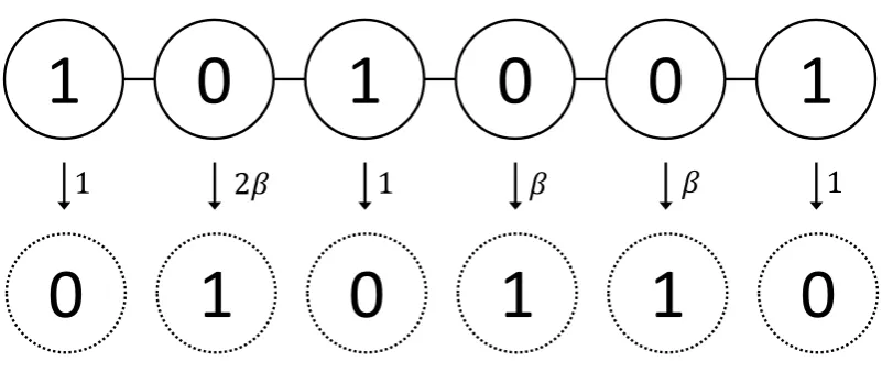
Liggett studied SIS epidemic model called contact processes on graphs with countable nodes [39]. A contact process is a continuous time Markov chain defined on{0,1}S _where_S_{is a countable set}

having a graph structure. In the graph structure, x∼yfor x,y∈S means that two nodesx andy are connected by an edge. The degree ofx is the number ofy∈Ssuch thaty∼x. In the contact process, degree of node is assumed to be finitely bounded. Forη∈ {0,1}Sandu∈S,η(u)∈ {0,1} representsu-th coordinates ofη. Denoteηx∈Sas flippingx-th coordinate fromη. In other words,

ηx(u) =η(u)ifu6=x and ηx(u) =1−η(u)ifu=x. (1.32)

For a given infection rateβ>0, the contact process is defined as

η→ηxat rate 





1 ifη(x) =1, β|{y:y∼x,η(y) =1}| ifη(x) =0.

(1.33)

(21)

1

0

1

0

1

0

1

0 2𝛽

1 𝛽

𝛽

1

[image:21.595.124.525.93.267.2]

1

Figure 1.3: The contact process on a 1-dimensional lattice. Solid circles represent current state. Dotted circles represent possible change of the current state.

IfS is finite,η eventually goes to all-zero state from the theory of finite state Markov chains. Liggett studied contact processes on thed-dimensional integer lattices. His results showed that there exists critical valueβcsuch that

• ifβ ≤βc, all-healthy distribution is the only invariant distribution, and the probability

distri-bution converges to it weakly for any initial distridistri-bution;

• ifβ >βc, there exists another invariant probability distributionν, and the probability

distri-bution converges toνweakly for any initial distribution.

One of the key differences of this contact process from classical model is that this process is defined on a discrete space{0,1}S_{. Draief, Ganesh et al. and Mieghem et al. applied a}

continuous-time Markov chain to model epidemic dynamics [16], [23], [42]. Ganesh et al. studied contact processes on finite graphs, focusing on how extinction time is related to graph structures.

(22)

1.2.3 Random Networks

Diseases are transmitted from one individual to another by contact, and the pattern of contact forms network whose structure gives a lot of effect for the dynamics of epidemics. In classical models, each individual has an equal chance of contact with others. Probably it is an unnatural assumption, but it provides a remarkable tractability: it allows one to represents a diffusion of disease by a differential equation, which can be solved analytically or numerically. In fact, we can go beyond this restriction by incorporating a full network structure into the model. The random graphs provide a good basis for doing this.

In network analysis, Erdös-Rényi model is one of the most important random graph models [19]. In theG(n,p)model, a graph is constructed by connectingnnodes randomly. Each edge is included in the graph with probability p, which is independent across the edges. An Erdös-Rényi random graph has a number of interesting properties as a model of a social network. For instance, the model shows a phase transition when p(n), the probability of connecting each nodes, as a function ofn, satisfies p(n) = c

n. A component is a subset of nodes in the social network that any two nodes are connected by a path consists of edges in the original social network. Ifc is small, we can expect that most nodes are disconnected from one another, and the size of each component is small, and vice versa. In fact, an Erdös-Rényi random graph has no components of size larger thanO(logn) with high probability ifc<1. On the contrary, most nodes have higher chance to be connected to each other ifcis large. Ifc>1, the Erdös-Rényi random graph has a giant component whose size isΘ(n) with high probability. Another interesting phenomenon is connectivity of random graphs.

Sharp threshold of connectivity on the Erdös-Rényi random graph isp(n) = log_nn. The Erdös-Rényi random graph has a pair of disconnected nodes with high probability if p(n) = clog_n n for c<1. Every pair of nodes is connected with high probability ifp(n) =clog_n nforc>1.

(23)

of connectivity on random geometric graph model satisfiesπr(n)2=clog_n nwithc=1. The random geometric graph is connected with high probability whenc>1, and it is not connected with high probability whenc<1. However, the random graph has bigger probability of existence of edge if two nodes consisting the edge are connected to a same node. It is different from Erd¨os-R´enyi random graph where the probability of existence for an edge is independent to each other.

With the comparison to real network model, a lot of random graph models describing real net-work have been proposed. One of them is “small-world” netnet-work. In the real netnet-works, many pairs of people are actually connected by a short chain of acquaintance. In other words, even though two particular people live far from each other, they can reach to the other with the small number of intermediates in the real networks. Watts and Strogatz suggested small-world network where the required number of intermediates in the chain from any two particular nodes is relatively smaller than one of Erdös-Rényi model [64]. In the small-world network, diseases will spread through a community much faster than Erdös-Rényi model. One of the real-world effect which Erdös-Rényi model does not provide is peer-effect. If two nodes are related to a particular node, the probability that two nodes are related is higher than arbitrary two nodes. Roughly speaking, if two people know a particular person, it is more likely that the two people know each other. The small world network also provides peer-effect.

One of the most important random graph models describing real world was suggested by Barab´asi and Albert [4]. The random graph constructed by the model is scale-free network whose degree is distributed according to a power law. In a scale-free network,P(k), the fraction of nodes connected tok other nodes satisfiesP(k)∼ k−γ _{asymptotically for constant}_{γ. This separates the}

(24)

1.2.4 Discrete Time Model

Continuous time model including classical SIR model and contact process assumes that the time period can be divided into infinitely small intervals. It is acceptable in various real world problems, however it is not in some situations. For example, consider a person living with family and working at company. He has more chance to contact with his family at night, but works at company and has more chance to contact with his colleagues during daytime. In this case, applying continuous time homogeneous model is not appropriate. Discrete time model is useful when dividing time interval into infinitely small pieces is not reasonable. Discrete time model is also useful when the interaction among the nodes are periodic. We can define unit interval as the period of the interaction.

A classic discrete time model of infectious disease transmission includes Reed-Frost model. In the classical Reed-Frost model, the disease is transferred directly from infected nodes to others. A susceptible node gets infected and is infectious to others only within the following time interval after contact with an infectious node. The contact probability between any two nodes are identical in the group within time interval. After a unit time interval, infectious nodes recover from the disease and become immune to the disease. Comparing to SIR model, a susceptible node in the class “S” gets infected after contact to infectious nodes. An infected node is in the class “I” and infectious to the susceptibles only within the unit time interval. After that, the infected node recovers and removed from epidemic dynamics in the class “R”.

At each timet, the number of infected nodes is denoted asCt, and the number of susceptibles

is denoted as St. The basic Reed-Frost model assumes homogeneity of risk of infection in the

network. Denote pas the probability of contact between any two nodes in the network, then 1−p is the probability that the two nodes do not have contact. A susceptible node does not get infected if the node does not have contact with any infected nodes during the unit interval of time. The model also assumes that the contact to each node is independent. We may use independence assumption to compute the probability of no contact to any of infected by multiplying the probabilities. We can then find the probability distribution of the number of infected nodes in the next generation.

P[Ct+1=k|Ct,St] =

St

k

(1−(1−p)Ct₎k ₍₁₋_p)CtSt−k _(1.34)

St+1, the number of susceptibles in the next generation is decided bySt+1=St−Ct+1.

(25)

al. applied fuzzy dynamical system to the Reed-Frost model for epidemic spreading taking into account uncertainties in the diagnostic of the infection[48].

The discrete time models also have been developed by admitting graph structure. Most of early works were conducted on the random graph model. Andersson studied stochastic process for exposing one or several given components of a random graph and applied the process to epidemic model[3]. Durrett studied how epidemic spread on networks commonly used in ecological models [17]. Chakrabarti et al. and Wang et al. suggested nonlinear epidemic map defined on fixed graph topology [10] [62]. Their research reveals that extinction and spread is deeply-related with the largest eigenvalue of adjacency matrix. Ahn et al. showed that the marginal probability of each node’s infection for given closed network converges and the limit point depends on the largest eigenvalue of the network [2].

1.2.5 Applications and Questions of Interest

Epidemic models can be applied to the other field. For example, there is a basic similarity between the spread of information and the transmission of infectious disease between the individuals. Both are processes in which spread is based on the contact. Huang et al. and Jacquet et al. studied the propagation speed of information on the network [28], [29]. Effective modification of graph structure on given condition to improve propagation speed is one of the interesting problems. The research on this topic can be applied to effective establishment of computer network.

Applying SIR model to rumors spreading, “S” represents the state where each individual has no information about the rumors if the person is in the state S. “I” represents the state where each in-dividual is exposed to the rumors and wants to transfer the rumors to acquaintances. “R” represents the state where each individual is not excited with the rumor any more. Each individual in the state R is tired from transferring the rumors and do not care any more. An interesting question on the size of people who are exposed to the rumors rises here. The size of eventual information holder distributes with particular probability distribution if probability model is admitted. The distribution depends on the topology of network, rate of converting each individual at the state S to the state I, and the rate from state I to R. Expected number of eventual information holder is well-defined if the probability on transition is defined. Asymptotic behavior of the expectation is an interesting question. Kenah et al. and Moore et al. applied percolation theory to study the infection of giant component in the graph [33], [45].

(26)

vaccination strategy vaccinates a fraction of the population randomly, using no knowledge of the network, however this is not an effective way. Cohen et al. and Madar et al. modified the random vaccination by vaccinating a higher degree nodes of randomly selected nodes [13], [40]. Miller et al. studied the effectiveness of targeted vaccination at preventing the spread of infectious disease by comparing vaccination strategies based on no information to complete information on the net-work [43]. Optimal vaccination strategy for given information is a topic many researchers are still working on.

On the contrary to the epidemic spread where one of the most important topic is how to prevent the disease to spread on the network, information diffusion focuses on how to spread the infor-mation. The idea is applied to viral marketing because a lot of people get information on goods from their friends or neighbors. The study to make the information on goods spread widely on the network. Phelps et al. and Richardson et al. studied viral marketing using epidmic model [53], [55].

Here is a short list of questions arising in epidemic spread.

• How the network topology affects the speed of information propagation? What is the effective way to modify network to improve the speed?

• What is the size of network exposed to the disease in the SIR model? Can we apply this to other epidemic models?

• How can we measure the effect of vaccination? What are the cost-effective vaccination algo-rithms?

• How can we apply epidemic model to the viral marketing? How can we measure the effect of the marketing?

• What is the dynamics of SIS epidemic models?

1.2.6 Contribution

The works on epidemic spreads in this thesis are conducted to answer the following questions :

• Can we study the global dynamics of the nonlinear epidemic model? Can we say what hap-pens when the linearized model is unstable?

(27)

In this dissertation, we analyze the various epidemic models. The main works are conducted on the discrete-time model. In the Chapter 3, we analyze the dynamics of the nonlinear epidemic map where domain represents each node’s marginal probability of being infected. The dynamics of epidemic map is simple when the epidemics dies out. The origin which represents the extinction of epidemics are globally stable. On the contrary to the previous work which focuses on the extinction of epidemics or how to eradicate epidemics, we analyze the dynamics of epidemics when the epi-demics do not die out. When the Jacobian matrix of the nonlinear map at the origin is not stable, the origin is an unstable fixed point of the nonlinear epidemic map. In the epidemic map proposed by Chakrabarti et al., there exists a unique nontrivial fixed point other than the origin. The nontrivial fixed point is globally stable, i.e., every point other than the origin converges to the nontrivial fixed point by time passes.

We also analyze the second model which admit immune effect. The immune-admitting model also has the unique nontrivial fixed point. However, the nontrivial fixed point in the immune-admitting model is not always stable. To analyze this, we give necessary and sufficient conditions for the nontrivial fixed point being locally stable. We apply the stability condition to the random graph families, and show that the nontrivial fixed point is locally stable with high probability if P[(d_min(n))2>a·dmax(n)]goes to 1 asn goes to infinity for any fixeda>0, whered(

n) min andd

(n) max are the minimum and the maximum degree of given random graph family withn vertices. The result can be applied to any random graph families. Since the degree distribution of Erd¨os-R´enyi model is concentrated on the expected degree, the nontrivial fixed point is locally stable with high probability. We propose a continuous time epidemic model. The continuous time model is based on the nonlinear epidemic map which is analyzed in the previous section. The origin is also an equilibrium point, and stability condition of the origin is same with one of the discrete time model. There also exists a unique nontrivial equilibrium point if the origin is unstable. The nontrivial fixed point is globally stable in the continuous time model even though the model is based on the immune-admitting model where stability of nontrivial fixed point is not guaranteed. To prove the stability, we suggest a Lyapunov function that is always decreasing except equilibrium points.

(28)

time, we study the “long enough time” which does not give any practical information. We give an upper bound of the probability that the epidemics does not die out until timetwhen the initial state is given.

To give a rigorous proof, we define a partial order which is defined on the set of the probability distributions on all the possible 2nstates. The upper bound is provided using the nonlinear epidemic map which is studied in the previous chapter. The nonlinear epidemic map is an approximation of the Markov chain model, and the upper bound shows that two models are closely related. With the upper bound, we provide a practical result that the mixing time is O(logn) if the origin is globally stable in the nonlinear epidemic map. TheO(logn) mixing time can be proved without the partial order which is necessary to give an upper bound of the survival probability using the nonlinear epidemic map. The alternative proof forO(logn)mixing time uses linear programming method. We apply this result to show that the Markov chain model based on the immune-admitting nonlinear epidemic map also has O(logn) mixing time if the origin is stable in the discrete time model.

(29)

Chapter 2 Random Riccati Equation

2.1 Introduction

In this chapter, we discuss geometric convergence of random Riccati recursions. We use superscript for time index in this chapter. Consider a linear time-varying state-space model of the form of







x(t+1)=F(t)x(t)+G(t)u(t) y(t+1)=H(t)x(t)+v(t)

E





u(t)

v(t)



 h

(u(t))T (v(t))T

i

=





Q(t) 0 0 R(t)



 (2.1)

wherex(t)∈_Rn_{is the unobserved state vector,}_y(t)_∈

Rmis them-dimensional observed measurement vector. u(t)∈_Rp_and_v(t)_∈

Rmare zero-mean white noises which represent process and measure-ment noise respectively.F(t)∈_Rn×n_,_G(t)_∈

Rn×p, andH(t)∈Rm×nare system matrices. The initial state of the system, x(0) is also considered to be zero-mean random vector which is independent from any ofu(t)andv(t).

It is well-known that optimal estimate ofx(t)can be recursively expressed as

ˆ

x(t+1)=F(t)xˆ(t)+F(t)P(t)(H(t))T(R+H(t)P(t)(H(t))T)−1(y(t)−H(t)xˆ(t)) (2.2)

In the time-invariant case, i.e.,

F(t)=F, G(t)=G, H(t)=H, Q(t)=Q, R(t)=R (2.3)

(30)

provided Kalman filter satisfies the following Riccati recursions :

P(t+1)=FP(t)FT−FP(t)HT(R+HP(t)HT)−1HP(t)FT+GQGT (2.4)

It is well-known thatP(t)in (2.4) converges if(F,G)is stabilizable and(F,H)is detectable. The pair(F,G)is called stabilizable if and only if there is no left eigenvector ofF, corresponding to an unstable eigenvalue ofF, that is orthogonal to G. The pair{F,H}is called detectable if and only if

{FT,HT}is stabilizable. [30]

We study the Riccati recursions when the regressor matrixH(t)is time-varying. We assume that H(t)is random matrix distributed according to a given distribution. Measuring average-eigenvalue distribution ofP(t)was studied by Vakili et al. [60]. We focus on convergence of probability distri-bution ofP(t). Specifically, we prove that the probability distribution ofP(t)converges geometrically fast.

In the next section, we describe the random Riccati recursions and the probability distribution of H(t), the regressor matrix. We also describe the general property of geometric convergence defining the distance between two probability measures. To get geometric convergence, we need to verify that the maximum distance between measures at particular time is strictly less than 1, which is the convergence rate. We show that the distance between any two probability distributions ofP(t) depending an initial point are strictly less than 1 after particular time depending on size of H(t). To prove this, we show that the probability distribution with any initial point has a common area of support which has strictly positive measure. We apply a well-known topological property that a continuous function defined in a compact space has a maximum. To apply this, we consider the probability distribution with an initial point as a map from an initial point to a measure space. We show that this is a continuous map. To get a compact space we compactifySn++, the space of positive definite matrices by admitting 0 and∞as eigenvalues of matrices. The main result is obtained by

combining all the intermediate results studied in this chapter.

2.2 Model Description

(31)

time-varyingHis defined as follows.

P(t+1)=FP(t)FT−FP(t)(H(t))T(R+H(t)P(t)(H(t))T)−1H(t)P(t)FT+Q (2.5)

P(0)∈_Sn

++,Q∈Sn++,R∈Sm++, andF ∈Rn×nin (2.5). mbynrandom matrixH(t)is the only factor that generates randomness of the system. We assume thatH(t) is independently and iden-tically distributed according to a given probability density function. We further assume that the probability distribution ofH(t)satisfies several conditions.

Definition 1 pH is a probability density function of H i.e., P[H(t)∈E] =REpH(H)dH for any

measurable set E⊂_Rm×n_{satisfying the following conditions.}

(a) The support of pHisRm×n. That is,P[H(t)∈E]>0if E has positive Lebesgue measure. (b) pH:Rm×n→R+is continuous.

(c) It decays faster than any polynomial. For any d>0, there exists Md such that pH(H)<

kHk−d

F for allkHkF >Md wherek · kF is Frobenius norm defined by square-root of all elements’

square-sum.

Example 2.2.1 A standard normal distribution pH(H) = (2π)−

mn

2 exp(−1 2kHk

2

F)is a distribution

satisfying all the conditions in definition 1.

We do not assume that each element ofH(t)is independent to each other.

Lemma 2.2.2 There are diagonal matrixR and random matricese He(t)which gives the same

proba-bility distribution to the system with R and H(t).

Proof: For fixedO, definee Re=ORe OeT. We can rewrite (2.5) withHe(t)=OHe (t)

P(t+1)=FP(t)FT−FP(t)(He(t))T(Re+He(t)P(t)(He(t)))T)−1He(t)P(t)FT+Q (2.6)

We can interpret that the probability distribution function of He(t) is rotated from one of H(t) by

multiplying the orthogonal matrixO. It is easy to see that the probability density function ofe He(t)

also satisfies all the conditions in definition 1. Moreover, the system withR,e He(t)and random Riccati

recursion withR,H(t)have the same probability distribution.

(32)

Definition 2 µ_P(t)is a probability measure such thatµ_P(t)(E) =P[P(t)∈E|P(0)=P].

µ_P(t)is the probability distribution ofP(t)where its initial point is given asP. It is necessary to define a metric on the space of probability measures to show geometric convergence of the probabil-ity measure. We show that the distance between any two initial probabilprobabil-ity distributions converges geometrically fast using the metric. We use the total variation distance.

Definition 3 For two measuresµ,ν, dTV(µ,ν) =supS|µ(S)−ν(S)|.

We define the support of µ_P(t)depending on an initial point. The support ofP(t)plays a central role in this chapter.

Definition 4 Supp(_Pt)is the support ofµ_P(t)when P(0)=P. That is, x∈Supp(_Pt)if and only if every open ball centered at x has positive measure underµ_P(t). In other words,

Supp(_Pt)={x∈_Sn

+:∀B(x,ε),µ (t)

P (B(x,ε))>0} (2.7)

2.3 General Property for Geometric Convergence

In this section, we describe how total variation distance of two probability measures decays geo-metrically fast. The material in this section is not only for random Riccati recursions, but for any random process. We follow the notation from [15].

Definition 5 P(t)(ζ,E) =P[P(t)∈E|P(0)=ζ]. M_E(t)=sup

ζ

P(t)(ζ,E),m(Et)=inf

ζ

P(t)(ζ,E).

The following inequality shows that the supremum of probability measure on particular mea-surable set depending on an initial point decreases as time passes.

M_E(t+l)=sup

α

P(t+l)(α,E) (2.8)

=sup

α

Z

P(l)(ξ,E)(P(t)(α,dξ)) (2.9)

≤sup

α

Z

M_E(l)(P(t)(α,dξ)) =M_E(l) (2.10)

(33)

· · · ≤m(_Et)≤m(_Et+l)≤ · · · ≤M_E(t+l)≤M_E(l)≤ · · · (2.11)

If lim

t→∞

M_E(t)=lim

t→∞

m(_Et)for every measurable setE, the probability measure converges to a steady state. The steady state is also a probability measure whose value onE is a limit ofm(_Et)andM_E(t).

M_E(t+l)−m(_Et+l) (2.12)

=sup

α,β

P(t+l)(α,E)−P(t+l)(β,E) (2.13) =sup

α,β

Z

P(l)(ξ,E)(P(t)(α,dξ)−P(t)(β,dξ)) (2.14)

≤ sup

α,β,S

Z

S

M_E(l)(P(t)(α,dξ)−P(t)(β,dξ)) +

Z

Scm

(l)

E (P

(t)_(α_,_dξ₎₋

P(t)(β,dξ)) (2.15) = sup

α,β,S

Z

S

(M_E(l)−m(_El))(P(t)(α,dξ)−P(t)(β,dξ)) (2.16)

=M_E(l)−m(_El) sup

α,β,S

P(t)(α,S)−P(t)(β,S)

!

(2.17)

Definition 6 π(t)=sup

α,β

dTV(µ( t)

α ,µ

(t)

β ) = sup α,β,S

P(t)(α,S)−P(t)(β,S)

We can interpretπ(t)as the maximum distance of probability distributions from any initial point at timet. Ifπ(t)<1 for particulart, then geometric convergence follows. It is obvious thatπ(t)≤1 for everyt. However, in many mathematical problems proving that supremum of some set where every element is less than or equal to 1 is strictly less than 1 is challenging.

2.4 Common Area of Support

π(t)=1 ifSupp(αt)andSupp

(t)

β are disjoint for someα,β. As a result, the system does not converge

geometrically fast if Supp(_αt) and Supp(t)

β are disjoint for some α,β. We investigate particulart

whereSupp(_αt)andSupp(t)

β have common area of the supports having positive probability measure.

We study the support ofP(t)for a given initial point. Specifically, we compareSupp_A(t)toSupp(_Bt) when the matrix Bis greater than A, i.e., B−A∈_Sn

(34)

monotone.

FBFT−FBHT(R+HBHT)−1HBFT− FAFT−FAHT(R+HAHT)−1HAF∈_Sn

+

ifB−A∈_Sn

+ (2.18)

Since Riccati equation is monotone, the maximal elements inSupp(_Bt)is greater thanSupp(_At)ifBis greater thanAi.e.,B−A∈Sn+. It is easy to see that the maximal element ofSupp

(1)

A isF

T_AF₊_Q.

IfF is nonsingular, monotonicity of the maximal element becomes strict. However, it is not trivial to check that whether the minimal element inSupp(_At)is always strictly smaller thanSupp(_Bt). We show that the minimal element ofSupp(_At) is inSupp_B(t)after finitet. As a result,Supp(_Bt)includes Supp(_At)after that. To give a proof, we suggest an algorithm to choose regresor matrixH(t)to make B(t)equal toA(t)for givenA(t).

R=diag(r0,· · ·,rm−1)without loss of generality by Lemma 2.2.2. For each row vector(H(t))j

such thatH(t)= ((H(t))T₀· · ·(H(t))T_m₋₁)T,

P(t)−P(t)(H(t))T(R+H(t)P(t)(H(t))T)−1H(t)P(t) = ((P(t))−1+H(t)R−1(H(t))T)−1= (P(t))−1+

m−1

∑

j=0 1 rj

(H(t))T_j(H(t))j !−1

(2.19)

DefineAkfork=am+bwithb∈ {0,1,· · ·,m−1}.

Ak= 

     

     

A if k=0,

Ak−1−

Ak−1hk−1hTk−1Ak−1

rk−1+hTk−1Ak−1hk−1 if m-k, FAk−1−

Ak−1hk−1hTk−1Ak−1

rk−1+hTk−1Ak−1hk−1

FT+Q if m|k,k>0.

(2.20)

Alm =P(l) by choosing P(0)=A, and rk =rb, hk = (H(a))Tb for all a∈ {0,· · ·,l−1}, b∈

{0,· · ·,m−1}.hkis a column vector while(H(a))bis a row vector. This describesAkwhen random

Hhas a realization.

(35)

suppose that realization ofHforBkis different from one forAk.

Bk=             

B if k=0,

Bk−1−

Bk−1gk−1gTk−1Bk−1

rk−1+gTk−1Bk−1gk−1 if m-k, F

Bk−1−

Bk−1gk−1gTk−1Bk−1

rk−1+gTk−1Bk−1gk−1

FT+Q if m|k,k>0.

(2.21)

We now claim that we can chooseg0,g1,· · ·,gn−1to makeBn=Anfor a givenAnwithB−A∈

Sn++.

We representAnas below forn=cm+dwithd∈ {0,1,2,· · ·,m−1}.

An=FcA(Fc)T− n−1

∑

k=0

Fdc−mke Akhkh

T kAk

rk+hTkAkhk

(Fdc−mke)T+

c−1

∑

a=0

FaQ(Fa)T (2.22)

We can representBnsimilarly.

We give a lemma which is useful to compute rank of a positive semidefinite matrix in the algo-rithm which will be given later.

Lemma 2.4.1 For C∈_Sn

+and v∈Rnsatisfying vTCv>0, the following statements hold.

C−Cvv

T_C

vT_Cv ∈S n

+ and rank

C−Cvv

T_C

vT_Cv

=rank(C)−1 (2.23)

Proof: DefineV0as null space ofC. It is obvious thatv∈/V0becausevTCv>0. We can choose V₁ such thatv∈V₁andRn=V0⊕V1 (V0andV1 don’t have to be orthogonal.) Then,<v1,v2>= vT₁Cv2is well-defined inner product onV1.

(C−Cvv

T_C

vT_Cv )v=Cv−Cv=0 (2.24)

The equation above guarantees that Null(C−CvvTC

vT_Cv)⊃ {v}. It is trivial to check that Null(C−

CvvT_C

vT_Cv)⊃Null(C). We get Null(C−

CvvT_C

vT_Cv)⊃Null(C)⊕ {v}.

For anyu∈Rn,u=u0+u1such thatu0∈V0,u1∈V1

uT(C−Cvv

T_C

vT_Cv )u=u T

1(C− CvvTC

vT_Cv )u1=

uT₁Cu1vTCv−uT₁CvvTCu1

vT_Cv ≥0 (2.25)

The equality holds only for u₁ =αv with some scalar α by the equality condition of Cauchy-Schwarz. That meansu∈Null(C)⊕ {v}ifu∈Null(C−CvvT_C

vT_Cv). Null(C−

CvvT_C

(36)

From the discussion above, Null(C−CvvT_C

vT_Cv ) =Null(C)⊕ {v}. It completes the proof.

We show thatSupp(_Bt)includesSupp_A(t)whenB−A∈Sn++by the following lemma. The lemma is based on the assumption thatF is nonsingular.

Lemma 2.4.2 Suppose that F∈Rn×nis nonsingular. For given A,B∈Sn++satisfying B−A∈Sn+

and h0,h1,· · ·,hn−1, it’s possible to find g0,g1,· · ·,gn−1such that Bn=An.

Proof: Define a symmetric matrixCkas below.

Ck=Fc(B−A)(Fc)T+ n−1

∑

j=0 Fdc−mje

AjhjhTjAj

rj+hT_jAjhj

(Fdc−mje)T−

k−1

∑

j=0 Fdc−mje

BjgjgTjBj

rj+gT_jBjgj

(Fdc−mje)T

(2.26) C₀is decided by given conditionA,Bandh₀,h₁,· · ·,hn−1.Ck fork>0 is determined by choosing

g0,g1,· · ·,gk−1. From the definition ofCk, it’s easy to verify that

Ck=Fdc−

k

me(B_k−_A_k)(Fdc− k me)T+

n−1

∑

j=k

Fdc−mje

AjhjhTjAj

rj+hTjAjhj

(Fdc−mje)T _(2.27)

We suggest an algorithm choosingg0,g1,· · ·,gn−1. Case 1. Ifn−k−rank(Ck)>0,gk=hk.

Case 2. If n−k−rank(Ck) =0, find gk satisfying the equation below for somev such that

vTCkv>0.

Fdc−mke Bkgkg

T kBk

rk+gT_kBkgk

(Fdc−mke₎T ₌Ckvv

T_C k

vT_C kv

(2.28) Before explaining how to findgksatisfying (2.28), we claim thatCk∈Sn+for everykby induction.

It is obvious that C0∈Sn+. Assume thatCk ∈S+n. Ifn− j−rank(Cj)>0 for every j≤k,

thengj=hj for all j≤kand it makesBk+1−Ak+1∈Sn+by the monotonicity of Riccati equation. Ck+1∈Sn+by (2.27) and rank(Ck+1) =rank(Ck)−1 or rank(Ck)becauseCk+1is justCkor a positive

semidefinite matrix whose rank is the same withCk minus rank-one positive-semi-definite matrix

by definition ofCk. Specifically,

Ck+1=Ck−Fdc−

k

me Akhkh

T kAk

rk+hTkAkhk

(Fdc−mke)T

orCk+1=FCkFT−Fdc−

k

me Akhkh

T kAk

rk+hT_kAkhk

(Fdc−mke)T _(2.29)

(37)

It is obvious that n−k−rank(Ck)≤0 atk=n. n−k−rank(Ck) goes down by 1 or stays in

Case 1 askincreases by 1. Sincen−k−rank(Ck)is non-positive at the end and it goes down by 1,

n−k−rank(Ck)should be zero at some particulark. It keeps staying at zero by Case 2 after that.

Eventually,n−k−rank(Ck) =0 atk=nand it’s equivalent to rank(Cn) =0. It means thatCn=0.

We find outg0,g1,· · ·,gk−1satisfyingBn=An.

It is enough to show that we can find outgk in Case 2. We defineC_k+ as pseudo-inverse ofCk.

(2.28) is satisfied ifCkv=Fdc−

k

meB_kg_k and the following equation is true :

rk+gTkBkgk=vTCkv=vTCkCk+Ckv=gTkBk(Fdc−

k me)TC+

k F

dc−k

meB_kg_k (2.30)

If we can findgk∈Rnsuch that

gT_k(Bk(Fdc−

k me)T_C+

k F

dc−k

me_B_k−_B_k)g_k>0 (2.31)

then we can makegksatisfying (2.30) by multiplying proper scalar togk.

DefineZk andDkas below.

Zk=B

1 2

k(F

dc−k

me)T D_k= (Z−1

k )

T_C

kZk−1∈S n

+ (2.32)

C+_k =Z_k−1D+_k(Z_k−1)T _{by property of pseudo-inverse matrix. (2.30) is equivalent to the following}

equation.

rk=gTk(Bk(Fdc−

k me₎T_C+

k F

dc−k me_B

k−Bk)gk (2.33)

= ((F−dc−mke₎T_g

k)T(ZkTZkCk+Z T

kZk−ZkTZk)((F−dc−

k me₎T_g

k) (2.34)

= ((F−dc−mke₎T_g

k)T(ZkT(D+k −In)Zk)((F−dc−

k me₎T_g

k) (2.35)

= (B 1 2

kgk)T(D+k −In)(B

1 2

kgk) (2.36)

The subscript ofInindicates thatInis then-dimensional identity matrix.

DefineXkas the following.

Xk= n−1

∑

j=k+1

Fdc−mje−dc− k me

AjhjhTjAj

rj+hT_jAjhj

(Fdc−mje−dc− k

(38)

In−Dk is represented usingXk as the following.

In−Dk= (Zk−1) T_Fdc−k

me

Ak−

AkhkhTkAk

rk+hTkAkhk

−Xk

(Fdc−mke)TZ−1

k (2.38)

=B− 1 2

k

Ak−

AkhkhTkAk

rk+hTkAkhk

−Xk

B− 1 2

k (2.39)

We know thatAk−

AkhkhTkAk

rk+hTkAkhk

∈_Sn

++. Defineαkas below.

αk=

A−_k1+ 1 rk

hkhTk

−1

then Ak−

AkhkhTkAk

rk+hT_kAkhk

−αkIn∈Sn+ (2.40)

DefineW as null space ofB− 1 2

k XkB

−1 2

k . For allw∈W,

wT(In−Dk)w=wTB

−1 2

k

Ak−

AkhkhTkAk

rk+hTkAkhk

B− 1 2

k w (2.41)

≥αkkB

−1 2

k wk

2 _(2.42)

≥αk(kB

1 2

kk

−1_k_w_k₎2 _(2.43)

= αk

kBkk

kwk2 _(2.44)

dim(W)≥k+1 becauseXk is summation ofn−k−1 rank-one positive-semi-definite matrices by

(2.37).

DefineV as span of eigenvectors ofDk corresponding to positive eigenvalues. Then, dim(V) =

rank(Dk) =rank(Ck) =n−kby assumption of Case 2.

There is nonzerou∈W∩V.

D 1 2 ku T

(D+_k −In) D 1 2 ku

=uTD 1 2

k(D

+

k −In)D

1 2

ku (2.45)

=uTu−uTDku (2.46)

=uT(In−Dk)u (2.47)

≥ αk

kBkk

kuk2>0 (2.48)

By choosinggkasB

−1 2

k D

1 2

kuwithuof proper norm, (2.30) holds. It completes the proof.

(39)

Theorem 2.4.3 If A,B∈_Sn

++satisfy B−A∈Sn+, then Supp (t)

A ⊂Supp

(t)

B for t≥ n m

Proof: Since the support of pHisRm×n,Btmwith anyg0,· · ·,gtm−1is in the support,Supp(

t)

B .

It is enough to show that we can find outg₀,g₁,· · ·,gtm−1such thatBtm=Atmfor any givenAtm.

First, we claim that it’s possible to find outg0,g1,· · ·,gn−1 such thatBn=An for givenA,B∈

Sn++satisfyingB−A∈Sn+andh0,h1,· · ·,hn−1. We already proved it for nonsingularFin Lemma 2.4.2.

For singular F, define F_ε =F+εIn. There is δ >0 such that Fε is nonsingular for all 0<

ε <δ. For each{εl}∞_l₌₁ converging to 0, we can find(g0,g1,· · ·,gn−1)which makesBn=An. If

(g0,g1,· · ·,gn−1)corresponding toεl converges to some point, the limit point makesBn=AnforF

and it’s exactly what we want.

If(g0,g1,· · ·,gn−1)corresponding toεl is bounded independent toεl, then they are in compact

space, and have convergent subsequence. The limit point of the subsequence is what we want. We prove the claim by showing that(g0,g1,· · ·,gn−1)of Lemma 2.4.2 hasε-independent upper bound. gk=B

−1 2

k D

1 2

ku, thenu T_(I

n−Dk)u=rk>0 by (2.36) and (2.47). u is also bounded since

uTu≤rkkBkk

αk

by (2.48).

kgkk2=gTkgk=uTD

1 2 kB −1 k D 1 2

ku (2.49)

≤ kB−_k1kkD 1 2

kuk

2₌_k_B−1

k k(u T

Dku) (2.50)

<kB−_k1kkuk2 _(2.51)

≤rkkBkkkB

−1

k k

αk

(2.52)

Since{εl}∞l=1 is sequence which is in(0,δ), kF+εlInkhas upper bound depending only onkFk

andδ. With that,kBkkhas an upper bound as below.

kBkk ≤ Fb k mc ε B(F bk mc ε ) T₊ bk mc−1

∑

a=0

F_εaQ(F_εa)T

(2.53)

Fork=am,kA−_k1k ≤ kQ−1k. Fork=am+bwith 0<b<m,

kA−_k1k=

A−_am1+

b−1

∑

j=0 1 rj

hjhTj

≤ kQ−1k+

b−1

∑

j=0

khjk2

rj

(40)

With that, _αk1 is upper bounded as below. 1 αk =

A−_k1+ 1 rk

hkhTk

≤ kA−_k1k+khkk 2

rk

(2.55)

In Case 1 of Lemma 2.4.2, gk is bounded because gk =hk, and Bk is also bounded by similar

inequality above.

We finish the proof by induction. It is obvious thatkB₀k,kB−₀1k,_α1

0 are bounded because they are determined by the given condition. Then, g0 also hasε-independent upper bound by (2.52). Assume thatgl andB−l 1haveε-independent upper bound for alll<k. Ifk=am,kB

−1

k k ≤ kQ

−1_k

andgkis also bounded by (2.52). Fork=am+bwith 0<b<m,

kB−_k1k=

B−_am1+

b−1

∑

j=0 1 rj

gjgTj

≤ kQ−1k+

b−1

∑

j=0

kgjk2

rj

(2.56)

gk is also bounded by (2.52). It completes the proof of the claim.

Choosing gk =hk for n≤k ≤tm−1 guarantee that Btm=Atm. It completes the proof of

Supp(_At)⊂Supp(_Bt).

It is obvious thatSupp(₀t), the support ofP(t)where an initial point is the zero-matrix, is same withSupp(_Qt−1). SinceSupp_A(t)⊃Supp(₀t)for any positive semidefinite matrixA, the following re-mark holds.

Remark 1 Supp(_At)⊃Supp_Q(t−1)for any A∈_Sn

+and t>mn+1

Supp(_Qt−1)is the common area of support at timetwith any initial point. Furthermore,Supp(_Qt−1) has nonzero probability measure for an initial point. The proof in this section requires the support ofHto be the wholemn-dimensional space to choose regressor vectors ofBeverywhere.

2.5 Computation of Probability Density Function

In this section, we compute probability density function using matrix calculus. From this section, we suppose thatF∈_Rn×n_{in (2.5) is nonsingular. We first study basic matrix calculus. We follow}

(41)

Definition 7 f(t)(P,·)is probability density function of measureµ_P(t)(·)i.e.,

µ_P(t)(E) =

Z

E

f(t)(P,C)dC (2.57)

IfFis singular, f(t)(P,·)is not defined. In this section, our goal is evaluating the actual value of f(t):Sn++×Sn++→R+. Roughly speaking, f(t)(P,C)is the probability density function ofP(t)=C givenP(0)=P.

Definition 8 For an arbitrary n×m matrix X ,dX denotes the exterior product of the mn elements ofdX

dX =

m

^

j=1

n

^

i=1

dxi j (2.58)

For a symmetric n by n matrix S,dS denotes the exterior product of the 1₂n(n+1)distinct elements ofdS

dS= ^ 1≤i≤j≤n

dsi j (2.59)

For a lower triangular n by n matrix L, dL denotes the exterior product of the 1₂n(n+1) lower triangular elements ofdL

dL= ^ 1≤j≤i≤n

dli j (2.60)

Lemma 2.5.1 If X=BY where X,Y are n×m matrices and B is a fixed nonsingular n×n matrix then

(dX) = (det(B))m(dY) (2.61)

Proof: It is Theorem 2.1.4 of [46]

Lemma 2.5.2 If S is an n×n positive definite matrix and S=LLT where L is lower-triangular with positive diagonal elements then,

(dS) =2n

n

∏

i=1

l_iin+1−i(dL) (2.62)

Lemma 2.5.3 Let Z be an a×b ( a≤b ) matrix of rank a and write Z=LO, where O is a×b matrix with OOT =Iaand L is an a×a lower-triangular matrix with positive diagonal elements.

Then

(dZ) =2n

a

∏

i=1

(42)

wheredO is volume element of Stiefel manifold Va,b={O∈Ra×b:OOT=Ia}

Remark 2

Vol(Va,b) =

Z

Va,b

dO= 2

a

πab/2

Γa(b/2)

where Γm(n) =π

m(m−1) 4

m

∏

i=1

Γ(n−1

2(i−1)) (2.64)

Definition 9 For fixed t satisfying mt>n,H¯ = [(H(0)₎T_(H(1)₎T _{· · ·}_(H(t−1)₎T_]_∈

Rn×mt. We rewrite ¯

H= [h¯0h¯1 · · · h¯mt−1].

µ_P(t)(E) =

Z

{H¯:P(0)₌_P_,_P(t)_∈_E_}p(¯ ¯

H)d ¯H (2.65)

where ¯p(H)¯ is probability density function of ¯H. ¯p(H) =¯ ∏lt−=10pH(H(

l)₎ _{by definition of the first} section thatH(l)is i.i.d.

DefineAkas in the previous section.

Ak=             

A if k=0,

Ak−1−

Ak−1h¯k−1h¯Tk−1Ak−1

rk−1+h¯Tk−1Ak−1h¯k−1 if m-k, F

Ak−1−

Ak−1h¯k−1h¯Tk−1Ak−1

rk−1+h¯Tk−1Ak−1h¯k−1

FT+Q if m|k,k>0.

(2.66)

It is obvious thatP(t)=AtmifP(0)=A.

Atm=FtA(FT)t− tm−1

∑

k=0

Fdt−mke Ak

¯ hkh¯TkAk

rk+h¯T_kAkh¯k

(FT)dt−mke+

t−1

∑

l=0

FlQ(FT)l (2.67)

Definition 10 Ψ1:Rn×tm→Rn×tmis defined byΨ1(H) =¯ G where¯

¯

gk= (G)¯ k=

1

q

rk+h¯T_kAkh¯k

Fdt−mkeA_kh¯_k (2.68)

Lemma 2.5.4 Ψ1is one-to-one.

(43)

Assume that ¯hl=h¯0l for everyl∈ {0,· · ·,k−1}, thenAk=A0kand

¯

gk=g¯0k ⇔

1

q

rk+h¯T_kAkh¯k

¯ hk=

1

q

rk+h¯0 T kAkh¯0_k

¯ h0

k (2.69)

⇔ _h¯0

k=αh¯k such that

1

q

rk+h¯TkAkh¯k

=q α

rk+α2h¯TkAkh¯k

(2.70)

⇔ h¯0_k=αh¯k and α=1 (2.71)

The discussion above holds fork=0. By induction, ¯hk=h¯0k for everykifΨ1(H) =¯ Ψ1(H¯0) We can rewrite (2.67) with ¯G.

Atm=FtA(FT)t− tm−1

∑

k=0 ¯ gkg¯Tk +

t−1

∑

l=0

FlQ(FT)l =FtA(FT)t−G¯G¯T+

t−1

∑

l=0

FlQ(FT)l (2.72)

Lemma 2.5.5 Ψ1(H)¯ is full-rank with probability 1

Proof: H¯ is full-rank with probability 1 because probability density function of ¯His continu-ous, and set of non-full-rank matrices is measure-zero. SinceΨ1is one-to-one by Lemma 2.5.4 and continuous, the range ofΨ1({H¯ : ¯His full-rank})has measure 1.

Lemma 2.5.6 If Z is a×b real matrix of rank a ( a≤b ) then Z can be uniquely written as Z=LO, where O is a×b matrix with OOT =Ia and L is an a×a lower-triangular matrix with positive

diagonal elements.

Proof: It is well-known as QR-decomposition.

Definition 11 For full-rankG¯ ∈_Rn×tm_,

Ψ2(G) = (L¯ ,O) where L is lower-triangular n×n matrix with positive diagonal elements, O∈Vn,tmand LO=G.¯

Ψ2(G)¯ is well-defined with probability 1 and it’s one-to-one in that case. It is enough to consider case of probability 1 on integration. We can rewrite (2.72) with(L,O).

Atm=FtA(FT)t−LOOTLT+ t−1

∑

l=0

FlQ(FT)l =FtA(FT)t−LLT+

t−1

∑

l=0

FlQ(FT)l (2.73)

Lemma 2.5.7

d ¯G=

tm−1

∏

k=0

(rk+h¯TkAkh¯k)−

n+2 2 _det(A

k)rk !

Random Propagation in Complex Systems: Nonlinear Matrix Recursions and Epidemic Spread

Matrix Recursions and Epidemic Spread

Acknowledgments

Abstract

Contents

Chapter 1

Introduction

1.1

Random Riccati Recursions

∑

1.2

Epidemic Spread

S

𝛽𝑆 𝑡 𝐼 𝑡

I

𝛾𝐼 𝑡

R

1

0

0

1

1

0

0

1

0

1

1

0

2𝛽

1

𝛽

𝛽

1

1

Chapter 2

Random Riccati Equation

2.1

Introduction

2.2

Model Description

2.3

General Property for Geometric Convergence

2.4

Common Area of Support

∑

∑

∑

∑

∑

∑

∑

∑

∑

∑

∑

∑

2.5

Computation of Probability Density Function

∏

∏

∏

∑

∑

∑

∑

∑

∑

∑

∏

_{𝛽𝑆 𝑡 𝐼 𝑡}

_{𝛾𝐼 𝑡}