based on interpolated FIR filters with adaptive interpolators in multipath channels
.
White Rose Research Online URL for this paper:
http://eprints.whiterose.ac.uk/3479/
Article:
de Lamare, Rodrigo C. and Sampaio-Neto, Raimundo (2007) Adaptive interference
suppression for DS-CDMA systems based on interpolated FIR filters with adaptive
interpolators in multipath channels. IEEE Transactions on Vehicular Technology. pp.
2457-2474. ISSN 0018-9545
https://doi.org/10.1109/TVT.2007.899931
[email protected] https://eprints.whiterose.ac.uk/
Reuse
Items deposited in White Rose Research Online are protected by copyright, with all rights reserved unless indicated otherwise. They may be downloaded and/or printed for private study, or other acts as permitted by national copyright laws. The publisher or other rights holders may allow further reproduction and re-use of the full text version. This is indicated by the licence information on the White Rose Research Online record for the item.
Takedown
If you consider content in White Rose Research Online to be in breach of UK law, please notify us by
Universities of Leeds, Sheffield and York
http://eprints.whiterose.ac.uk/
White Rose Research Online URL for this paper:
http://eprints.whiterose.ac.uk/3479
/
Published paper
de Lamare, Rodrigo C. and Sampaio-Neto, Raimundo (2008)
Adaptive
interference suppression for DS-CDMA systems based on interpolated FIR filters
with adaptive interpolators in multipath channels.
IEEE Transactions on Vehicular
Technology, 56 (5)
pp. 2457 - 2474
.
Adaptive Interference Suppression for DS-CDMA
Systems Based on Interpolated FIR Filters With
Adaptive Interpolators in Multipath Channels
Rodrigo C. de Lamare and Raimundo Sampaio-Neto
Abstract—In this paper, we propose an adaptive linear-receiver structure based on interpolated finite-impulse response (FIR) fil-ters with adaptive interpolators for direct-sequence code-division multiple-access (DS-CDMA) systems in multipath channels. The interpolated minimum mean-squared error (MMSE) and the in-terpolated constrained minimum-variance (CMV) solutions are described for a novel scheme, where the interpolator is rendered time-varying in order to mitigate multiple-access interference and multiple-path propagation effects. Based upon the interpolated MMSE and CMV solutions, we present computationally efficient stochastic gradient and exponentially weighted recursive least squares type algorithms for both receiver and interpolator filters in the supervised and blind modes of operation. A convergence analysis of the algorithms and a discussion of the convergence properties of the method are carried out for both modes of op-eration. Simulation experiments for a downlink scenario show that the proposed structures achieve a superior bit-error-rate convergence and steady-state performance to previously reported reduced-rank receivers at lower complexity.
Index Terms—Adaptive algorithms, direct-sequence code-division multiple access (DS-CDMA), multiuser detection, reduced-rank receivers.
I. INTRODUCTION
A
DAPTIVE linear receivers [1], [3], [4], [19] are a highly effective structure for combating interference in direct-sequence code-division multiple-access (DS-CDMA) systems since they usually show good performance and have simple adaptive implementation. The linear minimum mean-squared error (MMSE) receiver [3], [4] implemented with an adap-tive filter is one of the most prominent design criteria for DS-CDMA systems. Such a receiver only requires the timing of the desired user and a training sequence in order to suppress interference. Conversely, when a receiver loses track of theManuscript received June 27, 2005; revised March 22, 2006, July 4, 2006, February 2, 2007, and March 8, 2007. This work was supported by the Brazilian Council for Scientific and Technological Development (CNPq). The review of this paper was coordinated by Dr. M. Reed.
R. C. de Lamare was with Center for Studies in Telecommunications, Pontif-ical Catholic University of Rio de Janeiro, 22453-900 Rio de Janeiro, Brazil. He is now with the Communications Research Group, Department of Electronics, University of York, Y010 5DD York, U.K. (e-mail: [email protected]). R. Sampaio-Neto is with Center for Studies in Telecommunications, Pontif-ical Catholic University of Rio de Janeiro, 22453-900, Rio de Janeiro, Brazil (e-mail: [email protected]).
Color versions of one or more of the figures in this paper are available online at http://ieeexplore.ieee.org.
Digital Object Identifier 10.1109/TVT.2007.899931
desired user and a training sequence is not available, a blind linear minimum-variance (MV) receiver [5], [6] that trades off the need for a training sequence in favor of the knowledge of the desired user’s spreading code can be used to retrieve the desired signal.
The works in [1]–[6] were restricted to systems with short codes, where the spreading sequences are periodic. How-ever, adaptive techniques are also applicable to systems with long codes, provided some modifications are carried out. The designer can resort to chip equalization [7] followed by a despreader for downlink scenarios. For an uplink solution, channel-estimation algorithms for aperiodic sequences [8], [9] are required, and the sample average approach for estimating the covariance matrixR=E[r(i)rH(i)]of the observed data
r(i) has to be replaced by Rˆ =PPH+σ2I, which is
con-structed with a matrix P containing the effective signature sequence of users and the variance σ2 of the receiver noise
[10]. In addition, with some recent advances in random-matrix theory [11], it is also possible to deploy techniques originally developed for systems with short codes in implementations with long codes. Furthermore, the adaptive-receiver structures reported so far [1]–[10] can be easily extended to asynchronous systems in uplink connections. In the presence of large relative delays among the users, the observation window of each user should be expanded in order to consider an increased number of samples derived from the offsets among users. Alternatively, for small relative delays among users, the designer can utilize chip oversampling to compensate for the random-timing off-sets. These remedies imply in augmented filter lengths and, consequently, increased computational complexity.
In this context, a problem arises when the processing gain used in the system and the number of parameters for estimation is large. In these scenarios, the receiver has to cope with difficulties such as significant computational burden, increased amount of training and poor convergence, and tracking per-formance. In general, when an adaptive filter with a large number of taps is used to suppress interference, then it implies slow response to changing interference and channel condi-tions. Reduced-rank interference suppression for DS-CDMA [12]–[18] was originally motivated by situations where the number of elements in the receiver is large and where it is desirable to work with fewer parameters for complexity and convergence reasons. Early works in reduced-rank interference suppression for DS-CDMA systems [12]–[14] were based on
principal components (PC) of the covariance matrixRof the observation data. This requires a computationally expensive eigendecomposition to extract the signal subspace, which leads to poor performance in systems with moderate to heavy loads. An attempt to reduce the complexity of PC approaches was reported in [15] with the partial-despreading (PD) method, where the authors report a simple technique that allows the selection of the performance between the matched filter and the full-rank MMSE receiver. A promising reduced-rank technique for interference suppression, denoted as multistage Wiener filter (MWF), was developed by Goldstein et al. in [17] and was later extended to stochastic gradient (SG) and recursive adaptive versions by Honig and Goldstein in [18]. A problem with the MWF approach is that, although it is less complex than the full-rank solution, it still presents a considerable computational burden and numerical problems for implemen-tation. In this paper, we present an alternative reduced-rank interference-suppression scheme based on interpolated finite-impulse response (IFIR) filters with adaptive interpolators that gathers simplicity, great flexibility, low complexity, and high performance.
The IFIR filter is a single-rate structure that is mathemat-ically related to signal decimation followed by filtering with a reduced number of elements [20], [21]. The basic idea is to exploit the coefficient redundancy in order to remove a number of impulse-response samples, which are recreated using an interpolation scheme. The savings are obtained by interpolating the impulse response and by decimating the interpolated signal. This technique exhibits desirable properties, such as guaranteed stability, absence of limit cycles, and low computational com-plexity. Thus, adaptive IFIR (AIFIR) filters [22], [23] represent an interesting alternative for substituting classical adaptive FIR filters. In some applications, they show better convergence rate and can reduce the computational burden for filtering and coefficient updating, due to the reduced number of adaptive elements. These structures have been extensively applied in the context of digital filtering, although their use for parameter estimation in communications remains unexplored.
Interference suppression with IFIR filters and time-varying interpolators with batch methods, which require matrix inver-sions, were reported in [24]. In this paper, we investigate the suppression of multiple-access interference (MAI) and inter-symbol interference (ISI) with AIFIR filters (that do not need matrix inversions) for both supervised and blind modes of operation in synchronous DS-CDMA systems with short codes. A novel AIFIR scheme, where the interpolator is rendered adaptive, is discussed and designed with both MMSE and MV design criteria. The new scheme, introduced in [25] and [26], yields a performance superior to conventional AIFIR schemes [22], [23] (where the interpolator is fixed) and a faster conver-gence performance than full-rank and other existing reduced-rank receivers. Computationally efficient SG and recursive least squares (RLS)-type adaptive algorithms are developed for the new structure based upon the MMSE and MV performance criteria with appropriate constraints to mitigate MAI and ISI and jointly estimate the channel. The motivation for the novel structure is to exploit the redundancy found in DS-CDMA sig-nals that operate in multipath, by removing a number of samples
of the received signal and retrieving them through interpolation. The gains in convergence performance over full-rank solutions are obtained through the reduction of the number of parameters for estimation, leading to a faster acquisition of the required statistics of the method and a smaller misadjustment noise provided by the smaller filter [1], [19]. Furthermore, the use of an adaptive interpolator can provide a time-varying and rapid means of compensation for the decimation process and the discarded samples. The novel scheme has the potential and flexibility to consistently yield faster convergence than the full-rank approach, since the designer can choose the number of adaptive elements during the transient process and, upon convergence increase, the number of elements up to the full-rank. Unlike PC techniques, our scheme is very simple because it does not require eigendecomposition, and its performance is not severely degraded when the system load is increased. In contrast to PD, the AIFIR structure jointly optimizes two filters, namely, the interpolator and the reduced-rank, resulting in reduced-rank filters with fewer taps and faster convergence than PD since the interpolator helps with the compensation of the discarded samples. In comparison with the MWF, the proposed scheme is simpler, more flexible, and more suitable for implementation, because the MWF has numerical problems in fixed-point implementations.
A convergence analysis of the algorithms and a discussion of the global convergence properties of the method, which are not treated in [24]–[26], are undertaken for both modes of operation. Specifically, we study the convergence properties of the proposed joint adaptive interpolator and receiver scheme and conclude that it leads to an optimization problem with multiple global minima and no local minima. In this regard and based on the analyzed convergence properties of the method, we show that the prediction of the excess MSE of both blind and supervised adaptive algorithms is rendered possible through the study of the MSE trajectory of only one of the jointly opti-mized parameter vectors, i.e., the interpolator or the reduced-rank filters. Then, using common assumptions of the adaptive filtering literature, such as the independence theory, we analyze the trajectory of the mean tap vector of the joint optimization of the interpolator and the receiver and MSE trajectory. We also provide some mathematical conditions, which explain why the new scheme with SG- and RLS-type algorithms is able to converge faster than the full-rank scheme. Although the novel structure and algorithms are examined in a synchronous downlink scenario with periodic signature sequences in this paper, it should be remarked that they can be extended to long codes and asynchronous systems, provided that the de-signer adopts the modifications explained in the works reported in [7]–[11].
Fig. 1. Proposed adaptive reduced-rank receiver structure.
II. DS-CDMA SYSTEMMODEL
Let us consider the downlink of a synchronous DS-CDMA system withKusers,Nchips per symbol, andLppropagation
paths. The signal broadcasted by the base station intended for userkhas a baseband representation given by
xk(t) =Ak ∞
i=−∞
bk(i)sk(t−iT) (1)
wherebk(i)∈ {±1}denotes theith symbol for userk, the
real-valued spreading waveform, and the amplitude associated with user k are sk(t) and Ak, respectively. The spreading
wave-forms are expressed bysk(t) =Ni=1ak(i)φ(t−iTc), where ak(i)∈ {±1/
√
N},φ(t)is the chip waveform,Tc is the chip
duration, andN=T /Tcis the processing gain. Assuming that
the receiver is synchronized with the main path, the coherently demodulated composite received signal is
r(t) = K
k=1
Lp−1
l=0
hl(t)xk(t−τl) +n(t) (2)
where hl(t) and τl are, respectively, the channel coefficient
and the delay associated with the lth path. Assuming that
τk,l=lTc, the channel is constant during each symbol interval,
and the spreading codes are repeated from symbol to symbol, the received signalr(t)after filtering by a chip-pulse matched filter and sampled at chip rate yields the M =N+Lp−1
dimensional received vector
r(i) =H(i) K
k=1
AkSkbk(i) +n(i) (3)
wheren(i) = [n1(i)· · ·nMi)]Tis the complex Gaussian noise
vector withE[n(i)nH(i)] =σ2I, where(·)Tand(·)Hdenotes
transpose and Hermitian transpose, respectively, and E[.] is the expected value; the kth user symbol vector is bk(i) = [bk(i+Ls−1)· · ·bk(i)· · ·bk(i−Ls+ 1)]T, whereLsis the
ISI span, and the((2Ls−1)×N)×(2Ls−1)matrixSkwith
nonoverlapping shifted versions of the signature of userkis
Sk=
sk 0 · · · 0
0 sk . .. 0
..
. ... . .. ...
0 · · · sk
(4)
where the signature sequence for the kth user is sk= [ak(1)· · ·ak(N)]T, and the M ×((2Ls−1)×N) channel
matrixH(i)is
H(i) =
h0(i) · · · hLp−1(i) · · · 0 0
0 h0(i) · · · hLp−1(i) · · · 0
..
. . .. . .. . .. . .. ...
0 0 · · · h0(i) · · · hLp−1(i)
(5) where hl(i) =hl(iTc)forl= 0, . . . , Lp−1. The MAI arises
from the nonorthogonality between the received signals, whereas the ISI spanLsdepends on the length of the channel
response, which is related to the length of the chip sequence. For Lp= 1, Ls= 1 (no ISI), for 1< Lp N, Ls= 2, for N < Lp2N,Ls= 3, and so on.
III. LINEARINTERPOLATEDCDMA RECEIVERS
The underlying principles of the proposed CDMA-receiver structure are detailed here. Fig. 1 shows the structure of an IFIR receiver, where an interpolator and a reduced-rank re-ceiver that are time-varying are employed. TheM×1received vector r(i) = [r(0i)· · ·r(Mi)−1]T is filtered by the interpolator
filter vk(i) = [vk,(i)0· · ·v (i)
k,NI−1]
T, yielding the interpolated
re-ceived vectorrk(i). The vectorrk(i)is then projected onto an M/L×1vector¯rk(i). This procedure corresponds to
remov-ingL−1samples ofrk(i)of each set ofLconsecutive ones.
Then, the inner product of ¯rk(i) with the M/L-dimensional
vector of filter coefficients wk(i) = [w(k,i)0· · ·w (i)
k,M/L−1] T is
computed to yield the outputxk(i).
The projected interpolated observation vector ¯rk(i) =
Drk(i)is obtained with the aid of the M/L×M projection
matrixD, which is mathematically equivalent to signal decima-tion on theM×1 vectorrk(i). An interpolated receiver with
decimation factorLcan be designed by choosingDas
D=
1 0 0
..
. ... ...
0 · · · 0
(m−1)Lzeros
0 0 · · ·
.. . ... ...
1 0 · · ·
0 0 0 0 0
..
. ... ... ... ...
0 0 0 0 0
..
. ... ... ... ... . .. ...
0 0 0 0 0 · · · 0
(M/L−1)Lzeros
.. .
1
..
. ... ...
0 . . . 0
wherem(m= 1,2, . . . , M/L)denotes themth row. The strat-egy that allows us to devise solutions for both interpolator and receiver is to express the estimated symbolxk(i) =wkH(i)¯rk(i)
as a function ofwk(i)andvk(i)[we will drop the subscriptk
and symbol index(i)for ease of presentation]
xk(i) =w∗0vkHr˙0+w∗1vkHr˙1+· · ·+w∗M/L−1vHkr˙M/L−1
=vHk(i)r˙(0i)| · · · |r˙(M/Li) −1wk∗(i)
=vHk(i)ℜ(i)w∗k(i) (7) whereuk(i) =ℜ(i)wk∗(i)is anNI ×1 vector, theM/L
co-efficients ofwk(i)and theNI elements ofvk(i)are assumed
to be complex, the asterisk denotes complex conjugation, and
˙
rs(i)is a lengthNI segment of the received vectorr(i)
begin-ning atrs×L(i), and
ℜ(i) =
r(0i) rL(i) · · · r((iM/L) −1)L
r(1i) r (i)
L+1 · · · r (i)
(M/L−1)L+1
..
. ... . .. ...
r(Ni)I−1 r (i)
L+NI−1 · · · r (i)
(M/L−1)L+NI−1
. (8)
The interpolated linear-receiver design is equivalent in deter-mining an FIR filterwk(i)withM/Lcoefficients that provide
an estimate of the desired symbol
ˆ
bk(i) = sgn
RewHk(i)¯rk(i)
(9) whereRe(·)selects the real part,sgn(·)is the signum function, and the receiver parameter vectorwkis optimized according to
a selected design criterion.
A. MMSE Reduced-Rank Interpolated Receiver Design
The MMSE solutions forwk(i)andvk(i)can be computed
if we consider the optimization problem whose cost function is
JMSE(wk(i),vk(i)) =E|bk(i)−vHk(i)ℜ(i)w∗k(i)|2
(10) where bk(i) is the desired symbol for user k at time index (i). By fixing the interpolatorvk(i)and minimizing (10) with
respect towk(i), the interpolated Wiener filter/receiver weight
vector is
wk(i) =α(vk) = ¯Rk−1(i)¯pk(i) (11)
where R¯k(i) =E[¯rk(i)¯rHk(i)], p¯k(i) =E[bk∗(i)¯rk(i)], and ¯
rk(i) =ℜT(i)vk∗(i), and by fixingwk(i)and minimizing (10)
with respect tovk(i), the interpolator weight vector is
vk(i) =β(wk) =R−uk1(i)puk(i) (12)
whereRuk(i) =E[uk(i)u H
k(i)],puk(i) =E[b∗k(i)uk(i)], and
uk(i) =ℜ(i)w∗k(i). The associated MSE expressions are J(vk) =JMSE(α(vk),vk)
=σb2−p¯Hk(i)R−k1(i)¯pk(i) (13) JMSE(wk,β(wk)) =σb2−pHuk(i)R
−1
uk(i)puk(i) (14)
where σ2
b =E[|b(i)|2]. Note that points of global
minimum of (10) can be obtained by vk,opt=
arg minvkJ(vk) and wk,opt=α(vk,opt) or wk,opt=
arg minwkJMSE(wk,β(wk)) and vk,opt=β(wk,opt). At
the minimum point, (13) equals (14), and the MMSE for the proposed structure is achieved. We remark that (11) and (12) are not closed-form solutions forwk(i)andvk(i), since (11)
is a function of vk(i), and (12) depends onwk(i), and thus,
it is necessary to iterate (11) and (12) with an initial guess to obtain a solution, as in [24]. An iterative MMSE solution can be sought via adaptive algorithms.
B. CMV Reduced-Rank Interpolated Receiver Design
The interpolated CMV receiver parameter vectorwkand the
interpolator parameter vectorvkare obtained by minimizing
JMV(wk,vk) =E
|xk(i)|2
=EvHk(i)ℜ(i)w∗k(i)2
=wkH(i) ¯Rkwk(i) =vHk(i)Rukvk(i) (15)
subject to the proposed constraints CHkDHwk(i) =g(i) and vk(i)= 1, where the M ×Lp constraint matrix Ck
con-tains one-chip shifted versions of the signature sequence of user k; g(i) is an Lp-dimensional parameter vector to be
determined. The vector of constraints g(i) can be chosen among various criteria, although, in this paper, we adopt
g(i) as the channel parameter vector (g= [h0· · ·hLp−1] T)
because it provides better performance than other choices, as reported in [6]. The proposed constraint vk(i)= 1
en-sures adequate design values for the interpolator filter vk,
whereas CHkDHwk(i) =g(i) avoids the suppression of the
desired signal. By fixing vk, taking the gradient of the
La-grangian function Jl
MV(wk,vk) =E[[|vHk(i)ℜ(i)w∗k(i)|2] + Re[(CHkDHwk(i)−g(i))Hλ], whereλis a vector of Lagrange
multipliers, with respect towkand setting it to0, we get
E¯rk(i)¯rHk(i)
wk(i) +DCkλ=0
=⇒wk(i) = −R¯−k1(i)DCkλ.
Using the constraint CHkDHwk(i) =g(i) and
substitut-ing wk(i) =−R¯−k1(i)DCkλ, we arrive at λ= −(CHkDHR¯−k1(i)DCk)−1gk(i). The resulting expression
for the receiver is
wk(i) =αo(vk)
= ¯Rk(i)−1DCkCHkDHR¯k(i)−1DCk−
1
g(i) (16)
and the associate minimum output variance is
Jo(vk) =JMV(αo(vk),vk) =wHk(i) ¯Rk(i)wk(i)
=gH(i)CHkDHR¯k(i)−1DCk−
1
g(i). (17)
By fixingwk, the solution that minimizes (15) is
vk(i) =βo(wk) = arg min v
subject tovk(i)= 1. Therefore, the solution for the
interpo-lator is the normalized eigenvector ofRukcorresponding to its
minimum eigenvalue, via singular-value decomposition (SVD). As occurring with the MMSE approach, we iterate (16) and (18) with an initial guess to obtain a CMV solution [24]. Note also that (16) assumes the knowledge of the channel parameters. However, in applications where multipath is present, these parameters are not known, and thus, channel estimation is required. To blindly estimate the channel, we use the method of [6], [27]
ˆ
g(i) = arg min g
gHCHkR−m(i)Ckg (19)
subject to gˆ= 1, where R(i) =E[r(i)rH(i)], and m is a finite power and whose solution is the eigenvector corre-sponding to the minimum eigenvalue of the Lp×Lp matrix
CTkR(i)−mC
k through SVD. Note that, in this paper, we
restrict the values ofmto 1, although the performance of the channel estimator and, consequently, of the receiver can be improved by increasing m. In the next section, we propose iterative solutions via adaptive algorithms.
IV. ADAPTIVEALGORITHMS
We describe SG and RLS algorithms [31, Ch. 9 and 13] that adjust the parameters of the receiver and the interpolator based on the MMSE criterion and the constrained minimization of the MV cost function [25], [26]. The novel structure, as shown in Fig. 1 and denoted as INT, for the receivers gathers fast con-vergence, low complexity, and additional flexibility, since the designer can adjust the decimation factorLand the length of the interpolatorNI, depending on the needs of the application and
the hostility of the environment. Based upon the MMSE and CMV design criteria, the proposed receiver structure has the following modes of operation: training mode, where it employs a known training sequence; decision directed mode, which uses past decisions in order to estimate the receiver parameters; and blind mode, which is based on the CMV criterion and trades off the training sequence against the knowledge of the signature sequence. The complexity, in terms of arithmetic operations of the algorithms associated with the INT and the existing techniques, is included as a function of the number of adaptive elements for comparison purposes.
A. Least Mean Squares (LMS)Algorithm
Given the projected interpolated observation vector ¯rk(i)
and the desired symbolbk(i), we consider the following cost
function:
JMSE=|bk(i)−vHk(i)ℜ(i)w∗k(i)|2. (20)
Taking the gradient terms of (20) with respect to wk(i)
and vk(i) and using the gradient descent rules [31, Ch. 9,
pp. 367–371],wk(i+ 1) =wk(i)−µ∇JwMSE∗ andvk(i+ 1) =
vk(i)−η∇JvMSE∗ yields
vk(i+ 1) =vk(i) +ηe∗k(i)uk(i) (21)
wk(i+ 1) =wk(i) +µe∗k(i)¯rk(i) (22)
where ek(i) =bk(i)−wk(i)H¯rk(i) is the error for user k,
uk=ℜ(i)wk(i), andµandηare the step sizes of the algorithm
for wk(i) and vk(i). The LMS algorithm for the proposed
structure described in this section has a computational com-plexity O(M/L+NI). In fact, the proposed structure trades
off one LMS algorithm with complexity O(M) against two LMS algorithms with complexity O(M/L) and O(NI),
op-erating in parallel. It is worth noting that, to stabilize and to facilitate tuning of parameters, it is useful to employ normalized step sizes and, consequently, normalized least mean squares (NLMS)-type recursions when operating in a changing envi-ronment, and thus, we haveµ(i) =η0/¯rHk(i)¯rk(i)andη(i) = µ0/uHk(i)uk(i)as the step sizes of the algorithm forwk(i)and
vk(i), whereµ0andη0are the convergence factors.
B. RLS Algorithm
Consider the time average estimate of the matrix R¯k, as
required in (11), given by Rˆ¯k(i) =il=1αi−l¯rk(l)¯rHk(l),
where α (0< α1) is the forgetting factor that can be alternatively expressed byRˆ¯k(i) =αRˆ¯k(i−1) + ¯rk(i)¯rHk(i).
To avoid the inversion of Rˆ¯k(i)required in (11), we use the
matrix-inversion lemma and define Pk(i) = ˆ¯R −1
k (i) and the
gain vectorGk(i)as
Gk(i) =
α−1P
k(i−1)¯rk(i) 1 +α−1¯rH
k(i)Pk(i−1)¯rk(i)
(23)
and thus, we can rewritePk(i)as
Pk(i) =α−1Pk(i−1)−α−1Gk(i)¯rHk(i)Pk(i−1). (24)
By rearranging (23), we have Gk(i) =α−1Pk(i−1)¯rk(i)− α−1 G
k(i)¯rHk(i)Pk(i−1)¯rk(i) =Pk(i)¯rk(i). By employing
the least squares (LS) solution [a time average of (11)] and the recursionpˆk(i) =αpˆk(i−1) + ¯rk(i)b∗k(i), we obtain
wk(i) = ˆR¯ −1
k (i)ˆpk(i) =αPk(i)ˆpk(i−1)+Pk(i)¯rk(i)b∗k(i).
(25) Substituting (24) into (25) yields
wk(i) =wk(i−1) +Gk(i)ξk∗(i) (26)
where the a priori estimation error is described by
ξk(i) =bk(i)−wHk(i−1)¯rk(i). Similar recursions for the
interpolator are devised by using (12). The estimateRˆukcan be
obtained throughRˆuk(i) =
i
l=1αi−luk(l)uHk(l)and can be
alternatively written asRˆuk(i) =αRˆuk(i−1) +uk(i)u H
k(i).
To avoid the inversion of Rˆuk, we use the matrix-inversion
lemma, and, again, for convenience of computation, we define
Puk(i) = ˆR− 1
uk(i)and the Kalman gain vectorGuk(i)as
Guk(i) =
α−1P
uk(i−1)uk(i)
1 +α−1uH
k(i)Puk(i−1)uk(i)
and thus, we can rewrite (27) as
Puk(i) =α
−1P
uk(i−1)−α
−1G
uk(i)u H
k(i)Puk(i−1).
(28) By proceeding in a similar approach to the one taken to obtain (26), we arrive at
vk(i) =vk(i−1) +Guk(i)ξ∗k(i). (29)
The RLS algorithm for the proposed structure trades off a computational complexity of O(M2) against two RLS
algorithms operating in parallel, with complexityO((M/L)2)
andO(N2
I), respectively. BecauseNI is small (NI ≪M, as
will be shown later), the computational advantage of the RLS combined with the INT structure is rather significant.
C. CMV-SG Algorithm
Consider the unconstrained Lagrangian MV cost function
JMV=
vkH(i)uk(i)uHk(i)vk(i)
+λHCHkDHwk(i)−g(i)
+wHk(i)DCk−gH(i)
λ (30) where λis a vector of Lagrange multipliers. An SG solution can be devised by taking the gradient terms of (30) with respect to wk(i) and vk(i), as described by wk(i+ 1) =wk(i)− µw(i)∇Jwk(i) and vk(i+ 1) =vk(i)−η(i)∇Jvk(i), which
adaptively minimizes JMV with respect towk(i) andvk(i).
Substituting the gradient terms, the equations become
wk(i+ 1) =wk(i)−µw(i) (x∗k(i)¯rk(i) +DCkλ(i)) (31)
vk(i+ 1) =vk(i)−η(i)x∗k(i)uk(i) (32)
where xk(i) =wHk(i)¯rk(i) =vHk(i)uk(i). We use (32) and
can make vk(i+ 1)←vk(i+ 1)/vk(i+ 1) to update the
interpolator vk. It is worth noting that, in our studies, the
normalization on SG algorithms does not lead to different results from the ones obtained with a nonnormalized interpo-lator recursion. In this regard, analyzing the convergence of (32) without normalization is mathematically simpler and gives us the necessary insight into its convergence. By combining the constraint CkDHwk(i) =g(i) and (32), we obtain the
Lagrange multiplier
λ(i) = (CHkDHDCk)−1
×CHDwk(i)−µwCHDx∗k(i)¯rk(i)−g(i)
. (33)
By substituting (33) into (31), we arrive at the update rules for the estimation of the parameters of the receiverwk
wk(i+ 1) =Πk(wk(i)−µw(i)x∗k(i)¯rk(i))
+DCk
CHkDHDCk
−1
g(i) (34) whereΠk=I−DCk(CHkDHDCk)−1CHkDHis a matrix that
projectswkonto another hyperplane to ensure the constraints.
Normalized versions of these algorithms can be devised by substituting (32) and (34) into the MV cost function, differenti-ating the cost function with respect toµw(i)andµv(i), setting
them to zero, and solving the new equations. Hence, the CMV-SG algorithm proposed here for the INT receiver structure adopts the normalized step sizes µw(i) =µ0/¯rkH(i)Πk¯rk(i)
andη(i) =η0/uHkuk(i), whereµ0andη0are the convergence
factors forwkandvk, respectively.
The channel estimate ˆg(i) is obtained through the power method and the SG technique described in [27]. The method is an SG adaptive version of the blind channel-estimation algorithm described in (19) and introduced in [28] that requires only O(L2
p) arithmetic operations to estimate the
channel against O(L3
p) of its SVD version. In terms of
computational complexity, for the rejection of MAI and ISI, the proposed blind interpolated receiver trades off one blind algorithm with complexity O(M) against two blind algo-rithms with complexity O(M/L) and O(NI) operating in
parallel.
D. CMV-RLS Algorithm
Based upon the expressions for the receiverwkand
interpo-latorvkin (16) and (18) of the interpolated CMV receiver, we
develop a computationally efficient RLS algorithm for the INT structure that estimates the parameters ofwkandvk.
The iterative power method [29, pp. 405–408], [30, pp. 314–333] is used in numerical analysis to compute the eigenvector corresponding to the largest singular value of a matrix. In order to obtain an estimate ofvkand avoid the SVD
on the estimate of the matrixRuk(i), we resort to a variation of
the iterative power method to obtain the eigenvector ofRuk(i),
which corresponds to the minimum eigenvalue.
Specifically, we apply the power method to the difference betweenRuk(i)and the identity matrixIrather than applying it
to the inverse ofRuk(i). This approach, which is known as shift
iterations [30, p. 319], leads to computational savings on one or-der of magnitude, since direct SVD requiresO(N3
I), while our
approach needsO(N2
I). The simulations carried out reveal that
this method exhibits no performance loss. Hence, we estimate
Ruk(i) via the recursion Rˆuk(i) =
i
n=0αi−nuk(n)uHk(n)
and then obtain the interpolator vˆk with a one-step iteration
given by
ˆ
vk(i) =
I−νk(i) ˆRuk(i)
ˆ
vk(i−1) (35)
where νk(i) = 1/tr[ ˆRuk(i)]. After that, we make ˆvk(i)←
ˆ
vk(i)/vˆk(i) normalize the interpolator. This procedure is
based on the following result.
Lemma 1: LetRbe a positive semidefinite Hermitian sym-metric matrix andqminbe the eigenvector associated with the
smallest eigenvalue. Ifqminis unique and of unit norm, then,
withν = 1/tr[R], the sequence of vectorsv(i) = ˆv(i)/vˆ(i)
withvˆ(i) = (I−ν(i)R)ˆv(i−1)converges toqmin, provided
that vˆ(0) is not orthogonal to qmin. A proof is given in the
To recursively estimate the matrix R¯k(i)and avoid its
in-version, we use the matrix-inversion lemma and Kalman RLS recursions [31]
G(i) = α−
1Rˆ¯−1
k (i−1)¯rk(i) 1 +α−1¯rH
k(i) ˆR¯ −1
k (i−1)¯rk(i)
(36)
ˆ ¯
R−k1(i) =α−1R¯ˆ−k1(i−1)−α−1G(i)¯rHk(i) ˆR¯−k1(i−1) (37) where 0< α1 is the forgetting factor. The algorithm can be initialized withR¯−k1(0) =δIandR−1
uk(0) =δI, whereδis
a large positive number. For the computation of the reduced-rank receiver parameter vectorwk, we use the matrix-inversion
lemma [31] to estimate(CHkDHR¯k−1(i)DCk)−1, as given by
Γ−k1(i) = 1 1−α
×
Γ−k1(i−1)−Γ −1
k (i−1)γk(i)γkH(i)Γ−k1(i−1)
1−α α +γ
H
k(i)Γ−
1
k (i)γk(i)
(38)
where Γk(i) is an estimate of (CHkDHRˆ¯ −1
k (i)DCk), and γk(i) =CHkDHrk(i), and then, we construct the reduced-rank
receiver as
wk(i) = ˆ¯Rk(i)−1DCkΓ−k1(i)ˆg(i). (39)
The channel estimate gˆ(i) is obtained through the power method and the RLS technique described in [28]. Following this approach, the SVD on theLp×LpmatrixCkHR−1(i)Ck,
as stated in (19) and which requires O(L3
p), is avoided and
replaced by a single matrix–vector multiplication, resulting in the reduction of the corresponding computational complexity on one order of magnitude and no performance loss. In terms of computational complexity, the CMV-RLS algorithm with the interpolated receiver trades off one blind algorithm with complexity O(M2) against two with complexity O(M2/L2)
andO(N2
I)operating in parallel. SinceNIis small as compared
toM, it turns out that the new algorithms offer a significant computational advantage over conventional RLS algorithms.
E. Computational Complexity
In this section, we illustrate the computational complexity of the proposed INT structure and algorithms. In Table I, we consider supervised algorithms, whereas the complexity of blind algorithms is depicted in Table II. Specifically, we compare the full-rank, the proposed INT structure, the PD, the PC, and the MWF structures with SG and RLS algorithms.
In general, the INT structure introduces the term M/L, which can reduce the complexity by choosing the decima-tion factorL2. This is relevant for algorithms which have quadratic computational cost withM, i.e., the blind and trained RLS and the blind SG, because the decimation factor L in the denominator favors the proposed scheme which requires complexity O((M/L)2). This complexity advantage is not
verified with linear complexity recursions. For instance, with NLMS algorithms, the proposed INT has a complexity that is
TABLE I
COMPUTATIONALCOMPLEXITY OF
SUPERVISEDADAPTATIONALGORITHMS
TABLE II
COMPUTATIONALCOMPLEXITY OFBLINDADAPTATIONALGORITHMS
slightly superior to the full-rank. Among the other methods, the PD is slightly more complex than the INT. A drawback of PC methods is that they require an SVD with associated cost
O(M3) in order to compute the desired subspace. Although
the subspace of interest can be retrieved via computationally efficient tracking algorithms [13], [14], these algorithms are still complex(O(M)2)and lead to performance degradation as
compared to the actual SVD. The MWF technique has a com-plexityO(DM¯2), where the variable dimension of the vectors
¯
M =M −dvaries according to the orthogonal decomposition, and the rankd= 1, . . . , D.
In order to illustrate the complexity trend in a compre-hensive way, we depict in Fig. 2 curves which describe the computational complexity in terms of the arithmetic operations (additions and multiplications) as a function of the number of parameters M for recursive algorithms. For these curves, we consider Lp = 6 and assume that D is equal to M/2
Fig. 2. Complexity in terms of arithmetic operations versus number of received samples(M)for (a) supervised and (b) blind recursive adaptation algorithms.
computational cost of the algorithm of Song and Roy [14], which is capable of significantly reducing the cost required by SVD. In comparison with the existing reduced-rank techniques, the proposed INT scheme is significantly less complex than the PC and the MWF and is slightly less complex than the PD. This is because the analyzed algorithms have quadratic cost (PC with SVD has cubic cost), whereas the INT has complexity
O((M/L)2), as shown in Tables I and II.
V. GLOBALCONVERGENCEPROPERTIES OF THEMETHOD ANDCONVERGENCEANALYSIS OFALGORITHMS
In this section, we discuss the global convergence of the method and its properties, the trajectory of the mean tap vectors, of the excess MSE, and the convergence speed. Specifically, we study the convergence properties of the proposed joint adaptive interpolator and receiver scheme and conclude that it leads to an optimization problem with multiple global minima and no local minima. In this regard and based on the analyzed convergence properties of the method, it suffices to examine the MSE trajectory of only one of the jointly optimized parameter vectors (wk orvk) in order to predict the excess MSE of both
blind and supervised adaptive algorithms. We also provide a discussion of the speed of convergence of the INT, as compared to the full-rank.
A. Global Convergence of the Method and Its Properties
1)Interpolated MMSE Design: Let us first consider the trained receiver case and recall the associated MSE expressions in (13) and (14), namely, JMSE(vk,α(vk)) = J(vk) =σ2bk−p¯
H
k(i) ¯R−
1
k (i)¯pk(i) and JMSE(β(wk),wk) = σ2
bk−p¯ H
uk(i) ¯R
−1
uk(i)puk(i), where σ 2
bk=E[|bk(i)|
2]. Note
that points of global minimum of JMSE(wk(i),vk(i)) = E[|bk(i)−vHk(i)ℜ(i)w∗k(i)|2] can be obtained by vopt=
arg minvkJ(vk) and wopt=α(vopt) or wopt=
arg minwkJMSE(β(wk),wk) and vopt=β(wopt). At a
minimum point,JMSE(vk,α(vk))equalsJMSE(β(wk),wk),
and the MMSE for the proposed structure is achieved. We
further note that, sinceJ(vk) =J(tvk), for everyt= 0, then
if vk⋆ is a point of global minimum of J(vk), then tvk⋆ is
also a point of global minimum. Therefore, points of global minimum (optimum interpolator filters) can be obtained by
vk⋆= arg minvk=1J(vk). Since the existence of at least
one point of global minimum of J(vk) for vk= 1 is
guaranteed by the theorem of Weierstrass [32, Ch. 2, Sec. II-A, App. B], then the existence of (infinite) points of global minimum is also guaranteed for the cost function in (10).
In the context of global convergence, a sufficient but not necessary condition is the convexity, which is verified if its Hessian matrix is positive semidefinite, i.e., aHHa0,
for any vector a. First, let us consider the minimization of JMSE(wk(i),vk(i)) =E[|bk(i)−vHk(i)ℜ(i)w∗k(i)|2]with
fixed interpolators. Such optimization leads to the following Hessian H= (∂/∂wHk)((JMSE(.))/∂wk) =E[rk(i)rHk(i)] =
Rk(i), which is positive semidefinite and ensures the convexity
of the cost function for the case of fixed interpolators. Let us now consider the joint optimization of the interpolatorvk and
receiverwkthrough an equivalent cost function to (10)
˜
JMSE(z) =E
b−zHkBzk
2
(40)
where B=
0 0
ℜ 0
is an (NI+N/L)×(NI+N/L)
matrix, and the Hessian(H)with respect tozk = [wTkvTk]Tis
H = (∂/∂zHk)(∂( ˜JMSE(.))/∂zk) = E[(zHkBzk −bk)BH] + E[(zHkBHzk−b∗k)B] +E[BzkzHkBH] +E[BHzkzHkB]. By
examining H, we note that the third and fourth terms yield positive semidefinite matrices (aHE[BzkzHkBH]a0 and
aHE[BHz
kzHkB]a0,zk =0), whereas the first and second
terms are indefinite matrices. Thus, the cost function cannot be classified as convex. However, for a gradient search algorithm, a desirable property of the cost function is that it shows no points of local minimum, i.e., every point of minimum is a point of global minimum (convexity is a sufficient, but not necessary, condition for this property to hold), and it is conjectured that the problem in (40) has this property.
To support this claim, we carried out the following studies. 1) Let us consider the scalar case of the function in
(40), which is defined asf(w, v) = (b−w r v)2=b2−
2b w r v+ (wℜv)2, wherer is a constant. By choosing
v (the “scalar” interpolator) fixed, it is evident that the resulting function f(w, v) = (b−w c)2, where c is a
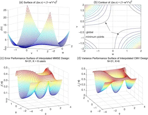
constant is a convex one, whereas for a time-varying interpolator, the curves shown in Fig. 3(a) and (b) indicate that the function is no longer convex but that it also does not exhibit local minima.
2) By taking into account that, for small interpolator filter length NI (NI 3),vk can be expressed in spherical
coordinates, and a surface can be constructed. Specifi-cally, we expressed the parameter vectorvk as follows:
vk=r[cos(θ) cos(φ) cos(θ) sin(φ) sin(θ)]T, where r is the radius, θ and φ were varied from −π/2 to
Fig. 3. (a) Error performance surface of the functionf(v, w) = (1−w∗r∗v)2. (b) Contour plots showing that the function does not exhibit local minima
and has multiple global minima. (c) Error performance surface of interpolated MMSE receivers atEb/N0= 15dB forL= 3. (d) Variance performance surface
ofJMV(v)for CMV receivers atEb/N0= 15dB forL= 2and channel with paths given by 0,−6, and−10 dB, spaced byTc.
J(vk), which is depicted in Fig. 3(c), reveals thatJ(vk)
has a global minimum value (as it should) but does not exhibit local minima, which implies that (40) has no local minima either. It should be noted that if the cost function in (40) had a point of local minimum, thenJ(vk)in (13)
should also exhibit a point of local minimum, even though the reciprocal is not necessarily true: A point of local minimum of J(vk) may correspond to a saddle point
of JMSE(vk,wk)if it exists. Note also that the latitude
X longitude plot in Fig. 3(c) depicts its two symmetric global minima in the unit sphere.
3) An important feature that advocates the nonexistence of local minima is that the algorithm always converge to the same minimum value, for a given experiment, independently of any interpolator initialization (except forv(0) = [0· · ·0]Tthat eliminates the signal) for a wide
range of SNR values and channels.
2)Interpolated CMV Design: For the blind case, let us first consider the minimization of JMV(wk(i),vk(i)) = E[|vHk(i)ℜ(i)w∗
k(i)|2] with fixed interpolators subject to
CHkDHwk(i) =g(i)andvk(i)= 1. It should be noted that
global convergence of the CMV method has been established in [6], and in this paper, we treat a similar problem when fixed
interpolators are used. Such optimization leads to the following Hessian H= (∂/∂wHk)((JMV(.))/∂wk) =E[rk(i)rHk(i)] =
Rk(i), which is positive semidefinite and ensures the convexity
of the cost function for the case of fixed interpolators.
Consider the joint optimization of the interpolator vk and
receiverwkvia an equivalent cost function to (10)
˜
JMV(z) =E
|zHkBzk|2
(41)
subject to CHkDHwk(i) =g(i), where B=
0 0
ℜ 0
is an
(NI+N/L)×(NI+N/L)matrix, and the Hessian (H), with
respect to zk= [wTkvkT]T, is H= (∂/∂zHk)(∂( ˜JMSE(.))/
∂zk) =E[zkHBzkBH] +E[zHkBHzkB] + E[BzkzHkBH] + E[BHzkzHkB]. By examining H, we note that, as it occurs
for the MMSE case, the third and fourth terms yield positive semidefinite matrices (aHE[BzkzHkBH]a0 and
aHE[BHzkzHkB]a0, zk=0), whereas the first and
problem in (41). Then, we carried out the following studies. 1) We have also plotted the variance performance surface of Jo(vk) in (17), depicted in Fig. 3(d). This surface
reveals that Jo(vk) has a global minimum (as it should)
but does not exhibit local minima, which implies that (41) subject to CHkDHwk(i) =g(i) has no local minima either.
2) Another important feature that suggests the nonexistence of local minima for the blind algorithms is that they always converge to the same minimum value, for a given experiment, independently of any interpolator initialization (except for
v(0) = [0· · ·0]Tthat eliminates the signal) for a wide range of
parameters.
B. Trajectory of the Mean Tap Vectors
This part is devoted to the analysis of the trajectory of the mean tap vectors of the proposed structure when operating in blind and supervised modes. In our analysis, we employ the so-called independence theory [1], [31, Ch. 9, pp. 390–404] that consists of four points.
1) The received vectorsr(1), . . . ,r(i)and their interpolated counterparts ¯rk(1), . . . ,¯rk(i) constitute a sequence of
statistically independent vectors.
2) At timei,r(i)and¯rk(i)are statistically independent of bk(1), . . . , bk(i−1).
3) At timei,bk(i)depends onr(i)andrk(i)but is
indepen-dent of previousbk(n), forn= 1, . . . , i−1.
4) The vectorsr(i)and¯rk(i)and the samplebkare mutually
Gaussian-distributed random variables (r. v.).
In the present context, it is worth noting that the indepen-dence assumption holds for synchronous DS-CDMA systems [1], which is the present case, but not for asynchronous models, even though it provides substantial insight.
1)Trained Algorithm: To proceed, let us drop the user k
index for ease of presentation and define the tap error vectors
ew(i)andev(i)at time indexi
ew(i) =w(i)−wopt, ev(i) =v(i)−vopt (42)
wherewoptandvoptare the optimum tap vectors that achieve
the MMSE for the proposed structure. Substituting the expres-sions in (42) into (21) and (22), we get
ew(i+ 1) =I−µ¯r(i)¯rH(i)ew(i) +µ¯r(i)e∗(i) (43)
ev(i+ 1) =I−ηu(i)uH(i)ev(i) +ηu(i)e∗(i). (44)
By taking expectations on both sides, we have
E[ew(i+ 1)] =
I−µR¯(i)E[ew(i)] +µE[¯r(i)e∗(i)]
(45)
E[ev(i+ 1)] = [I−ηRu(i)]E[ev(i)] +ηE[u(i)e∗(i)].
(46)
At this point, it should be noted that the two error vectors have to be considered together because of the joint optimization of the interpolator filter and the reduced-rank filter. Rewriting the terms E[¯r(i)e∗(i)] and E[u(i)e∗(i)] and using (42) and the
independence theory [31, Ch. 9, pp. 390–404], we obtain
E[¯r(i)e∗(i)] = ¯p(i)−E¯r(i)vT(i)ℜH(i)E[ew(i)]
−E¯r(i)woptT ℜ∗E[ev(i)]
−E¯r(i)wToptℜ∗vopt
(47)
E[u(i)e∗(i)] = ¯pu(i)−Eu(i)wT(i)ℜ∗(i)E[ev(i)]
−Eu(i)voptT ℜHE[ew(i)]
−Eu(i)wToptℜ∗vopt
. (48)
By combining (45)–(48), the trajectory of the error vectors is given by
E[ew(i+ 1)] E[ev(i+ 1)]
=A
E[ew(i)] E[ev(i)]
+B (49)
where we have the expression shown at the bottom of the next page, and
B=
µp¯(i)−µEr¯(i)wToptℜ∗vopt
ηp¯u(i)−ηEu(i)woptT ℜ∗vopt
.
Equation (49) implies that the stability of the algorithms in the proposed structure depends on the matrixA. For stability, the convergence factors should be chosen so that the eigenvalues of
AHAare less than one.
2)Blind Algorithm: The mean vector analysis of the blind algorithm is slightly different from [6], because our approach uses a decoupled SG channel-estimation technique [28] that yields better channel estimates. Hence, we consider the joint estimation of wk and vk, whileg is a decoupled estimation
process. To proceed, let us drop the user k index for ease of presentation and substitute the expressions of (42) into (32) and (34) that gives
ew(i+ 1)=
I−µ¯r(i)¯rH(i)ew(i)+DC(CHDHDC)−1g(i)
−µΠ¯r(i)vToptℜ∗(i)wopt
−µΠ¯r(i)wToptℜH(i)ev(i) (50)
ev(i+ 1)=
I−ηu(i)uH(i)ev(i)−ηu(i)vToptℜ∗(i)ew(i)
−ηu(i)woptT ℜ∗(i)vopt (51)
where Π=I−DC(CHDHDC)−1CHDH, and we used
the fact that the scalars have alternative expressions, as
(eTw(i)ℜH(i)vopt)T = (eTw(i)ℜH(i)vopt) =voptT ℜ∗(i)ew(i)
and (eT
v(i)ℜ∗(i)wopt)T= (eTv(i)ℜ∗(i)wopt) =wToptℜH(i)×
termµΠ¯r(i)voptℜ∗(i)wopt, we get
E[ew(i+ 1)] =
I−µR¯(i)E[ew(i)]
+DC(CHDHDC)−1E[g(i)]
−µΠE¯r(i)woptT ℜH(i)E[ev(i)] (52)
E[ev(i+ 1)] = [I−ηRu(i)]E[ev(i)]
−ηEu(i)vToptℜ∗(i)E[ew(i)]
−ηEu(i)woptT ℜ∗(i)vopt. (53)
By combining (52) and (53), the trajectory of the error vectors for the MV case is given by
E[ew(i+ 1)] E[ev(i+ 1)]
=AMV
E[ew(i)] E[ev(i)]
+BMV (54)
where
AMV=
I−µR¯(i) −µΠE¯r(i)woptT ℜH(i) −ηEu(i)vT
optℜ∗(i)
[I−ηRu(i)]
and
BMV=
DC(CHDHDC)−1E[g(i)]
−ηEu(i)woptT ℜ∗(i)vopt
.
Equation (54) suggests that the stability of the algorithms in the proposed structure depends on the matrix AMV. For
stability, the convergence factors should be chosen so that the eigenvalues ofAHMVAMVare less than one.
C. Trajectory of Excess MSE
Here, we describe the trajectory of the excess MSE at steady state of the trained and the blind SG algorithms.
1)Trained Algorithm: The analysis for the LMS algorithm using the proposed interpolated structure and the computation of its steady-state excess MSE resembles the one in [31, Ch. 9, pp. 390–404]. Here, an interpolated structure with joint op-timization of interpolator vk and reduced-rank receiver wk
is taken into account. Despite the joint optimization, for the computation of the excess MSE, one has to consider only the reduced-rank parameter vector wk because the MSE attained
upon convergence by (13) and (14) should be the same. Here, we will drop the userkindex for ease of presentation. Consider the MSE at timei+ 1as
ǫ(i+ 1) =Eb(i+ 1)−wH(i+ 1)¯r(i+ 1)2
. (55)
By using w(i+ 1) =wopt+ew(i+ 1), wopt, vopt and the
fact that the expressions in (13) and (14) are equal for the
optimal parameter vectors, the MSE becomes
ǫ(i+ 1) =σ2b−p¯H(i+ 1) ¯R−1(i+ 1)¯p(i+ 1)
−p¯H(i+ 1)ew(i+ 1)−eHw(i+ 1)¯p(i+ 1)
−wHoptp¯(i+ 1) +woptH R¯(i+ 1)wopt
+wHoptR¯(i+ 1)ew(i+ 1)
+eHw(i+ 1) ¯R(i+ 1)wopt
+Eew(i+ 1)¯r(i+ 1)¯rH(i+ 1)eHw(i+ 1)
=σ2b−p¯H(i+ 1) ¯R−1(i+ 1)¯p(i+ 1)
+Eew(i+ 1)¯r(i+ 1)¯rH(i+ 1)eHw(i+ 1)
=JMMSE(wopt,vopt) +ξexc(i+ 1) (56)
wherep¯(i+ 1) =E[b∗(i+ 1)¯r(i+ 1)],ǫ
min=JMMSE(wopt,
vopt) =σb2−p¯H(i+ 1) ¯R−1(i+ 1)¯p(i+ 1) is the MMSE
achieved by the proposed structure when we have wopt and
vopt, andξexc(i+ 1) =E[eHw(i+ 1)¯r(i+ 1)¯rH(i+ 1)ew(i+ 1)] is the excess MSE at time i+ 1. To compute the excess MSE, one must evaluate the termξexc(i+ 1). By invoking the
independence assumption and the properties of trace [31, Ch. 9, pp. 390–404], we may reduce it as follows:
EeHw(i+ 1)¯r(i+ 1)¯rH(i+ 1)ew(i+ 1)
= trR¯(i+ 1)K(i+ 1). (57) In the following steps, we assume that i is sufficiently large such that the matrix R¯(i) = ¯R(∞) = ¯R. To proceed, let us define some new quantities that will perform a rotation of coordinates to facilitate our analysis, as advocated in [31]. DefineQHRQ¯ =Λ, whereΛis a diagonal matrix consisting of the eigenvalues of R¯ and Q is the unitary matrix with the eigenvectors associated with these eigenvalues. Letting
QHKQ=X, we get
ξexc(i+ 1) = trRK¯ (i+ 1)= trQΛQHQX¯(i+ 1)QH
= trQΛX¯(i+ 1)QH= trΛX¯(i+ 1) (58) where we used the property of trace, and QHQ=I. Because
Λis a diagonal matrix of dimensionM/L, we have
ξexc(i+ 1) =
M/L
n=1
λnxn(i+ 1) (59)
wherexn,n= 1,2, . . . , M/Lare the elements of the diagonal
of X(i). Here, we may use (45) and invoke the independence
A=
(I
−µR¯)−µE¯r(i)vT(i)ℜH(i) −µE¯r(i)wToptℜ∗(i) −ηEu(i)voptT ℜH(i) (I−ηR¯u)−ηEu(i)wT(i)ℜ∗(i)
theory [31, Ch. 9, pp. 390–404] in order to describe the corre-lation matrix of the weight error vector
K(i+ 1) =Eew(i+ 1)eHw(i+ 1)
=I−µR¯(i)K(i)I−µR¯(i)+µ2ǫmin. (60)
Next, using the transformationsQHRQ¯ =Λ andQHKQ=
X, and similarly to [31, Ch. 9, pp. 390–404], a recursive equation in terms ofX(i)andΛcan be written as
X(i+ 1) = (I−µΛ)X(i)(I−µΛ) +µ2ǫminΛ (61)
Because of the structure of the above equation, one can de-couple the elements xn(i) from the off-diagonal ones, and
thus,ξexc(i+ 1)depends onxn(i), according to the following
recursion:
xn(i+ 1) = (1−µλn)2xn(i) +µ2ǫminλn. (62)
At this point, it can be noted that such a recursive relation converges, provided that all the roots lie inside the unit circle, i.e.,(1−µλn)2<1for alln, and thus, we have, for stability
0< µ < 2 λmax
(63)
where λmax is the largest eigenvalue of the matrix R¯. In
practice, tr[ ¯R] is used as a conservative estimate of λmax.
By taking limi→∞ on both sides of (62), we get xn(∞) = (µ/(2 +µλn))ǫmin. Then, taking limits on both sides of (59)
and usingxn(∞), we obtain the expression for the excess MSE
at steady state
ξexc(∞) =
M/L
n=1
λnxn(∞)
= M/L
n=1
µλn
2 +µλnǫmin= µ
2tr[ ¯R]
1−µ2tr[ ¯R]
ǫmin. (64)
The expression in (64) can be used to predict semianalytically the excess MSE, whereR¯ must be estimated with the aid of computer simulations, since it is a function of the interpola-tor v(i). Alternatively, one can conduct the analysis for the interpolatorv(i), which results in the expression ξexc(∞) =
((η/2)tr[Ru]/(1−(η/2)tr[Ru]))ǫmin, whereηis the step size
of the interpolator, the matrix Ru=Ru(∞), and Ru(i) = E[u(i)uH(i)], as defined in connection with (12). A more complete analytical result, which is expressed as a function of both step sizes µand η, and statistics of the noninterpolated observation vectorr(i)requires further investigation in order to determinetr[ ¯R(∞)], which depends onηortr[Ru(∞)], which depends on µ. Nevertheless, such investigation is beyond the scope of this paper, and it should be remarked that the results would not differ from the semianalytical results derived here [that implicitly take into account the parameters ofv(i)].
2)Blind Algorithm: Our algorithm is an MV technique, and its steady-state excess MSE resembles the approach in [6]. In the current context, however, an interpolated structure with joint optimization of interpolatorvk and reduced-rank receiver
wk is taken into account. In particular, it suffices to consider,
for the computation of the excess MSE, only the reduced-rank parameter vector wk, because the MSE attained upon
convergence by the recursions, that work in parallel forwkand
vk, should be the same. Here, we will drop the userkindex for
ease of presentation. Consider the MSE at timei+ 1as
ǫ(i+ 1) =Eb(i+ 1)−wH(i+ 1)¯r(i+ 1)2
. (65)
By usingw(i+ 1) =wopt+ew(i+ 1)and the independence
assumption, the MSE becomes
ǫ(i+ 1) =ǫmin−E
b(i+ 1)¯rH(i+ 1)ew(i+ 1)
−eHw(i+ 1)E[b∗(i+ 1)¯r(i+ 1)] +wHoptR¯(i+ 1)ew(i+ 1)
+eHw(i+ 1) ¯R(i+ 1)wopt+ξexc(i+ 1) (66)
whereǫmin=σb−E[b(i+ 1)¯rH(i+ 1)]wopt−woptH E[b∗(i+
1)¯r(i+ 1)] +wHoptR¯(i+ 1)woptis the MSE with the optimal
reduced-rank receiverwopt, and the optimal interpolatorvopt
and ξexc(i+ 1) =E[eHw(i+ 1) ¯R(i+ 1)ew(i+ 1)] is the
ex-cess MSE at timei+ 1. Sincelimi→∞E[ew(i)] =0, we have lim
i→∞ǫ(i+ 1) =ǫmin+ limi→∞ξexc(i+ 1). (67)
Note that the second term in (67) is the steady-state excess MSE due to adaptation, which is denoted byξ¯excand which is related
towby
¯
ξexc(∞) = lim
i→∞trE
¯
Rew(i+ 1)eHw(i+ 1)
. (68)
Let us define Re(i) =E[ew(i)eHw(i)] and Re= limi→∞Re(i), and use the property of trace to obtain
¯
ξexc(∞) = trE[ ¯RRe] = vecH( ¯R)vec(Re). (69)
At this point, it can be noted that to assess ξ¯exc(∞), it is
sufficient to studyRe, which depends on the trajectory of the
tap error vector. For simplicity and similarly to [6], we assume that eg(i)≈CHDHew(i), which is valid as the adaptation
approaches steady state. Using the expression ofew(i+ 1)and
taking expectation on both sides of ew(i+ 1)eHw(i+ 1), the
resulting matrixRe(i+ 1)becomes
Re(i+1)
≈Re(i)−µRe(i) ¯R(i)Π+ΠRR¯ e(i)
−µEΠew(i)woptH ¯r(i)¯rH(i)Π+Π¯r(i)¯rH(i)wopteHw(i)Π
+µ2EΠ¯r(i)¯rH(i)(woptwoptH +Re(i))¯r(i)¯rH(i)Π
(70)
where Π=I−DC(CHDHDC)−1CHDH. Since
limi→∞Re(i+ 1) =Re and limi→∞E[ew(i) =0, taking
limits on both sides of (70) yields
ReRΠ¯ +ΠRR¯ e
Here, an expression forξ¯exc(∞)can be obtained by using the
properties of the Kronecker product and arranging all elements of a matrix into a vector columnwise through the vec operation. Hence, the expression for the steady-state excess MSE becomes
¯
ξexc(∞) = tr[ ¯RRe] =µvecH( ¯R)T−1a (72)
whereT=( ¯RΠ)T⊗I+I⊗(ΠR¯)−µ[ΠT
⊗Π]E[(r(i)r(i)H)T⊗
(r(i)r(i)H)],a= [(Π)T⊗Π] E[(r(i)rH(i))T⊗(r(i)rH(i))]
vec(woptwHopt), and⊗accounts for the Kronecker product. The
expression in (72) can be used to predict, semianalytically, the excess MSE, where the matricesR¯ andTand the vectoraare computed through simulations.
D. Transient Analysis and Convergence Speed
With regard to convergence speed, adaptive receivers/filters have a performance which is proportional to the number of adaptive elementsM [1], [19], [31]. Assuming stationary noise and interference, full-rank schemes with RLS algorithms take
2M iterations to converge, while SG algorithms require at least an order of magnitude more iterations than RLS techniques [31]. In addition, it is expected that RLS methods do not show excess MSE (whenα= 1and operating in a stationary environ-ment), and its convergence is independent of the eigenvalues of the input correlation matrix.
With the proposed INT reduced-rank scheme, the conver-gence can be made faster due to the reduced number of filter coefficients, and the decimation factorLcan be varied in order to control the speed and ability of the filter to track changing environments. As given in the Appendix, we mathematically explain how the INT structure can obtain gains in convergence speed over full-rank schemes with SG and RLS algorithms, respectively.
For SG algorithms, the analysis of the transient components given in the Appendix of the INT scheme reveals that the speed of convergence depends on the eigenvalue spread of the reduced-rank covariance matrix. In principle, we cannot mathematically guarantee that the INT always converges faster than the full-rank, but several studies that examine the eigen-value spread of the full-rank and the INT covariance matrix show that, for the same data, the INT structure is able to consistently reduce the eigenvalue spread found in the original data covariance matrix, thus explaining its faster convergence in all analyzed scenarios.
For RLS techniques, the analysis of the transient components given in the Appendix guarantees mathematically that the INT is able to converge faster due to the reduced number of filter elements, and we show that the INT with the RLS converges in about2M/Literations, as compared to the full-rank, which requires2M iterations.
VI. SIMULATIONS
In this section, we investigate the effectiveness of the pro-posed linear-receiver structure and algorithms via simulations and verify the validity of the convergence analysis undertaken for predicting the MSE obtained by the adaptive algorithms. We
have conducted experiments under stationary and nonstationary scenarios to assess the convergence performance in terms of signal-to-interference-plus-noise ratio (SINR) of the proposed structure and algorithms and compared them with other recently reported techniques, namely, adaptive versions of the MMSE [19] and CMV [6] full-rank methods, the eigendecomposition (PC) [12], [13], the PD [15], and the MWF [18] reduced-rank techniques with reduced-rank D. Moreover, the bit-error-rate (BER) performance of the receivers employing the analyzed techniques is assessed for different loads, processing gains
(N), channel paths (Lp) and profiles, and fading rates. The
DS-CDMA system employs Gold sequences of lengthN = 31
andN = 63.
Because we focus on the downlink, users experiment under the same channel conditions. All channels assume that Lp= 6 as an upper bound (even though the
effec-tive number of paths will be indicated in the experi-ments). For fading channels, the channel coefficients hl(i) = plαl(i)(l= 0,1,2), where lL=1p p2l = 1, andαl(i) is a
com-plex unit variance Gaussian random sequence obtained by passing complex white Gaussian noise through a filter with approximate transfer function c/1−(f /fd)2, where c is a normalization constant, fd=v/λc is the maximum
Doppler shift, λc is the wavelength of the carrier
fre-quency, and v is the speed of the mobile [33]. This proce-dure corresponds to the generation of independent sequences of correlated unit power Rayleigh r. v. (E[|α2
l(i)|] = 1).
The phase ambiguity derived from the blind channel-estimation method in [28] is eliminated in our simulations by using the phase ofg(0)as a reference to remove the ambiguity, and for fading channels, we assume ideal phase tracking and express the results in terms of the normalized Doppler frequencyfdT
(cycles per symbol). Alternatively, differential modulation can be used to account for the phase rotation. For the proposed interpolated receivers structures, we employM = (N+Lp− 1)/Ladaptive elements forL= 2,3,4,and8, and whenM is not an integer, we will approximate it to the nearest integer. For the full-rank receiver, we haveM = (N+Lp−1).
In the following experiments, the type of adaptive algorithms used and their mode of operation, i.e., training mode, decision-directed mode, and blind mode, are indicated. For the training-based algorithms, the receiver employs training sequences with
Ntr symbols and then switches to decision-directed mode.
The full-rank receiver is considered with the NLMS and RLS techniques, the interpolated receivers are denoted INT, the PC method [12] requires an SVD on the full-rank covariance matrix, and the subspace dimension is chosen asD=K. For the PD approach, the columns of the projection matrix are nonoverlapping segments ofsk, as described in [15], whereas,
INT, uses the CMV-SG and CMV-RLS algorithms particularly designed for it. The different receiver techniques, algorithms, processing gainN, the decimation factorL, and other param-eters are depicted in the legends. The eigendecomposition-based receiver of Wang and Poor [13] is denoted subspace W and P and employs an SVD to compute its eigenvectors and eigenvalues. With regard to blind channel estimation, we employ the method in [28] for all SG-based receivers, whereas for the RLS-based receivers, we adopt the study in [28]. The blind MWF and its adaptive versions (blind MWF-SG and blind MWF-rec) [18] have their rankDoptimized for each situation and employ the blind channel estimation in [28] to obtain the effective signature sequence in multipath. For the RAKE receiver [33], we also employ the SG blind channel estimation of [28] when compared to other SG-based multiuser receivers, whereas for the comparison with RLS-based receivers, we use its RLS version [28].
A. MSE Convergence Performance: Analytical Results
Here, we verify that the results (64) and (72) of the section on convergence analysis of the mechanisms can provide a means of estimating the excess MSE. The steady-state MSE between the desired and the estimated symbol obtained through simulation is compared with the steady-state MSE computed via the expressions derived in Section VI. In order to illustrate the usefulness of our analysis, we have carried out some ex-periments. The interpolator filters were designed withNI = 3
elements, and the channels have three paths with gains 0,−6, and−10 dB, respectively, where, in each run, the delay of the second path(τ2)is given by a discrete uniform r. v. between one
and four chips, and the third path is computed with a discrete uniform r. v. between one and(5−τ2)chips in a scenario with
perfect power control.
[image:16.594.307.552.69.232.2]In the first experiment, we have considered the LMS algorithm in trained mode and tuned the parameters of the mechanisms, in order to achieve a low steady-state MSE upon convergence. The parameters of convergence, i.e.,µ, are 0.05, 0.06, 0.075, and 0.09 for the full-rank and the INT with L= 2,3,and4, respectively, andη= 0.005for the interpolator with allL. The results are shown in Fig. 4(a) and indicate that the analytical results closely match those obtained through sim-ulation upon convergence, verifying the validity of our analysis. In the second experiment, we have considered the blind SG algorithm and tuned the parameters of the mechanisms, in order to achieve a low steady-state MSE upon convergence, similarly to the LMS case. The chosen values forµare 0.0009, 0.001, 0.0025, and 0.004 for the full-rank and the INT with L= 2,3,and4, respectively, andη= 0.005for the interpolator with allL. The curves depicted in Fig. 4(b) reveal that a discrep-ancy is verified in the beginning of the convergence process, when the estimated covariance matrix is constructed with few samples. In addition, this mismatch between the theoretical and simulated curves is explained by the fact that blind algorithms are noisier than trained techniques [5]. However, as time goes by and the data record is augmented, the statistics of the signals is acquired, and the modeled and simulated MSE curves come to a greater agreement.
Fig. 4. MSE convergence for analytical and simulated results versus number of received symbols using (a) trained LMS algorithms and (b) blind SG algorithms.
Fig. 5. Design of interpolator filters to obtain the best dimensions forNI with random three-path channel parameters (r. v. between−1 and 1) as given
in Section IV-A, where the scenario has equal power users. (a) Trained RLS-type algorithms atEb/N0= 12dB. (b) Blind CMV-RLS-type algorithms at
Eb/N0= 15dB.
B. SINR Convergence Performance
The SINR at the receiver end is used here to assess the convergence performance of the analyzed methods. In the fol-lowing experiments, we will assess the SINR performance of the analyzed adaptive receiver techniques and their correspond-ing algorithms, namely, the proposed interpolated receiver, the PC, the PD, the MWF, and the RAKE. We remark that the parameters of the algorithms have been tuned in order to optimize performance, and the receiver parameters have been carefully chosen to provide a fair comparison among the analyzed methods.
First, let us consider the issue of how long should be the interpolator filter. Indeed, the design of the interpolator filter is a fundamental issue in our approach because it affects its convergence and BER performance. In order to obtain the most adequate dimension for the interpolator filter vk, we
conducted experiments with values ranging from NI = 3 to NI = 6, which correspond to the ones shown in Fig. 5 for the
[image:16.594.310.552.283.459.2]