Adaptive regression and model selection in data mining problems

(1)

THESES SIS/LIBRARY TELEPHONE: +61 2 6125 4631

R.G. MENZIES LIBRARY BUILDING NO:2 FACSIMILE: +61 2 6125 4063

THE AUSTRALIAN NATIONAL UNIVERSITY EMAIL: [email protected]

CANBERRA ACT 0200 AUSTRALIA

USE OF THESES

This copy is supplied for purposes

of private study and research only.

Passages from the thesis may not be

copied or closely paraphrased without the

(2)

School of Mathematical Sciences

THE AUSTRALIAN NATIONAL UNIVERSITY

Canberra, Australia

Adaptive Regression and Model

Selection in Data Mining

Problems

by

Sergey Bakin

A thesis submitted for the degree of Doctor of Philosophly of The Australian National University.

(3)

11

Statement

I declare that this thesis is my own original work and all sources have been acknowledged.

(4)

111

Acknowledgments

I would like to express my profound gratitude to my supervisor Professor Michael R. Osborne as well as to my advisor Doctor Markus Hegland for the time and efforts they have put into directing and supervising my PhD research, for the fruitful discussions we have had, for their patience in dealing with my written English, and for their invaluable assistance in helping me to get an academic appointment.

I would like to thank Doctor Steven Roberts for discussing various research problems with me as well as for writing a reference letter to support my job application. I would also like to thank the CRC for Advanced Computational Systems (ACSys) for the generous financial and technical assistance.

I must acknowledge the support given to me by my mother whose love and strength have enabled me to concentrate on my studies.

Special thanks to Jacki Wicks who has made the last month of my stay at ANU pleasant and unforgettable, as well as to Derek Holtby who has greatly influenced the formation of my spiritual outlook and has set an example of living as a Christian for me. I am also deeply grateful to James Rice and Csaba Schneider for their support and friendship.

I would like to thank all the students and staff of the School of Mathematical Sciences of the Australian National University, and members of the Advanced Computation Group in particular, for the friendly and stimulating working and social environment.

(5)

lV

Abstract

Data Mining is a new and rapidly evolving area which deals with problems related to extracting structure from massive commercial and scientific data sets. Regression analysis is one of the major Data Mining techniques. The data sets encountered in the Data Mining area are often characterized by a large number of attributes (variables) as well as data records. This imposes two major requirements on the regression analysis tools used in Data Mining: first, in order to produce accurate and parsimonious models exhibiting the most important features of the problem in hand, they should be able to perform model selection adaptively and, second, the cost of running such tools has to be reasonably low. Most of the modern regression tools fail to meet the above requirements. This thesis is intended to contribute to the improvement of the existing methodologies as well as to propose new approaches.

We focus on two regression estimation techniques. The first one, called Probing Least Absolute Squares Modelling (PLASM), is a generalization of the Least Absolute Shrinkage and Selection Operator (LASSO) by R. Tibshirani which minimizes the residual sum of squares subject to the 11-norm of the regression coefficients being less than a constant.

LASSO has been shown to enjoy stability of the ridge regression coupled with the ability to carry out model selection. In our approach called PLASM, we replace the constraint employed in LASSO with a different constraint. PLASM allows for an arbitrary grouping of basis functions in a model and includes LASSO as a special case. The implication of using the new constraint is that PLASM is able to perform model selection in terms of groups of basis functions. This turns out to be very useful in a number of data analytic problems. For example, as far as additive modelling is concerned, the dimensionality of the PLASM minimization problem is much less than that of LASSO and is independent

(at least explicitly) of the number of datapoints which makes it suitable for use in the Data Mining context.

(6)

v

(7)

CONTENTS

Statement

Acknowledgments

Abstract

1 Introduction

1.1 Problem Formulation . . . . 1.2 Modern Regression Modelling Procedures 1.3 Overview of the Contents of the Thesis . .

2 Probing Least Absolute Squares Modelling 2.1 Least Absolute Shrinkage and Selection Operator 2.2 Introduction of PLASM

2.3 Regularized PLASM . .

2.4 Kuhn-Tucker Conditions for the Regularised PLASM .

3 New Formulation of PLASM 3.1 New Regularised PLASM . 3.2 New Form of the Original PLASM

4 Investigation of PLASM & Numerical Issues 4.1 The Orthogonal Design Case . . . . .

4.2 Highly Constrained PLASM Solutions 4.3 PLASM as a GCV Minimizer . . 4.4 Bayesian Formulation of PLASM 4.5 Numerical Solution of PLASM . 4.6 Optimal Value for the Parameter t' .

4.7 Experiments with PLASM involving Synthetic Data 4.8 Application of PLASM to Real Data . . . . 4.9 PLASM and Second-Order Cone Programming

(8)

CONTENTS

5 PLASM and Penalized Least Squares 5.1 Penalized Least Squares

5.2 Modified PLASM . . . .

5.3 New Formulation of the Modified PLASM 5.4 Case of Positive Semidefinite Matrices K;

6 Probing Least Absolute Deviations Modelling 6.1 Introduction of PLADM

6.2 Regularized PLADM . .

6.3 Kuhn-Tucker Conditions for the Regularized PLADM

7 New Form of Regularized PLADM

7.1 New PLADM Optimization Problem . . . . 7.2 Properties of the New PLADM Optimization Problem 7.3 PLADM and the Iteratively Reweighted PLASM

8 Multivariate Adaptive Regression Splines 8.1 Friedman's MARS . . . . 8.2 MARS algorithm based on B-splines 8.3 Computational Complexity of BMARS . 8.4 Parallel BMARS . . . .

9 BMARS: Implementation Issues 9.1 Smoothing of BMARS Models. 9.2 Least Squares Fit Procedure . . 9.3 Logistic Regression with Offset

10 Numerical Experiments with BMARS 10.1 Synthetic Datasets . . .

10.2 Modelling "Hard" Dataset .

10.3 Case Study: NRMA Claims Data . 10.4 Scalability of the Parallel BMARS

11 Convergence of a Greedy Algorithm 11.1 Adaptive Least Squares Procedure 11.2 General Properties of ALS . . . 11.3 Estimation of the Convergence Ratio

vu 70 71

74

77

81 81 84 85 91 91 94 . 101

104

. 105 . 109 . 112 . 115

118

. 118 . 120 . 121

125

. 125 . 128 . 130 . 134

136

(9)

CONTENTS

12 Conclusion

12.1 Overview of the Main Results 12.2 Future Work . . . .

A A Short User's Guide to BMARS

Bibliography

Vlll

145

. 145 . 147

150

(10)

LIST OF FIGURES lX

List of Figures

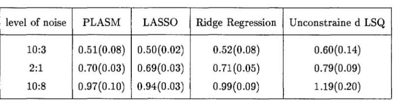
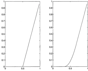
4.1 Graphs of (centered) univariate terms of additive model by PLASM in real

data example (datapoints are shown by dots) . . . 69

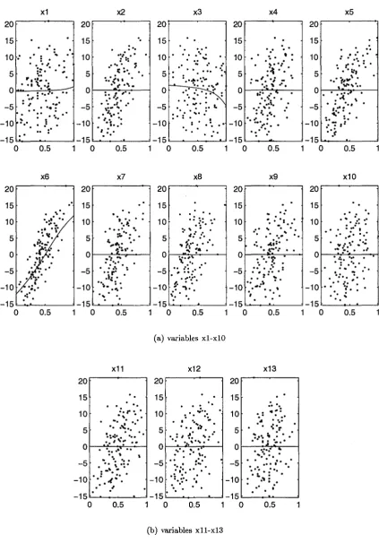
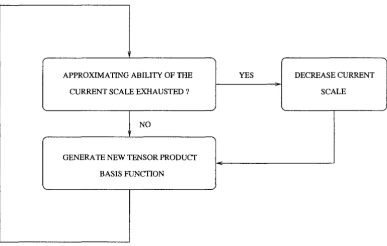
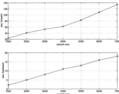
8.1 Modified forward stepwise procedure of BMARS. . 112

8.2 Complexities of the forward and backward parts of BMARS as functions of

the size of a sample (dataset). . . 113

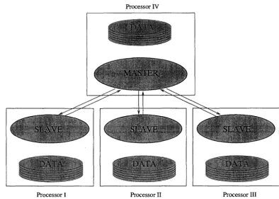
8.3 The diagram of the parallel BMARS. . . 116

9.1 Smoothing of a truncated power basis function.

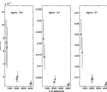
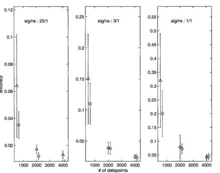
10.1 Average SMSE levels of models of the function (10.1) by MARS (circles) and BMARS (triangles) for various dataset sizes and signal-to-noise ratios

. 119

(whiskers span ave(SMSE)

±

usMSE intervals) . . . 127

10.2 Average SMSE levels of models of the function (10.2) by MARS (circles) and BMARS (triangles) for various dataset sizes and signal-to-noise ratios (whiskers span ave(SMSE)

±

usMSE intervals) . . . 128

10.3 Average SMSE levels of models of the function (10.3) by MARS (circles) and BMARS (triangles) for various dataset sizes and signal-to-noise ratios (whiskers span ave(SMSE)

±

usMSE intervals) . . . 129 10.4 Average SMSE levels of models of the function (10.4) by MARS (circles)

and BMARS (triangles) for various dataset sizes and signal-to-noise ratios (whiskers span ave(SMSE)

±

usMsE intervals). . . . . 130

10.5 Average SMSE levels of models of the function (10.5) by MARS (circles) and BMARS (triangles) for various dataset sizes and signal-to-noise ratios

(whiskers span ave(SMSE)

±

usMSE intervals). . 131

10.6 Modelling of a hard dataset in section (10.2). . . 132

(11)

LIST OF TABLES x

List of Tables

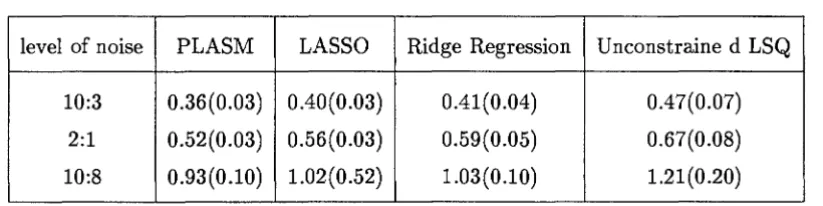
4.1 Prediction Errors along with the corresponding standard deviations (in parentheses) of models of the function

f

1(x) in (4.19). . . 63

4.2 Prediction Errors along with the corresponding standard deviations (in parentheses) of models of the function

h(x)

in (4.19). . . 63 4.3 Results (percentage of models having the correct structure) of modelling

the function

fi(x)

in (4.19). . . 64 4.4 Results (percentage of models having the correct structure) of modelling

the function

h(x)

in (4.19). . . 64 4.5 Prediction Errors along with the corresponding standard deviations (in

parentheses) of models of the function f3(x) in (4.19). . . 65

(12)

CHAPTER 1. INTRODUCTION 1

Chapter

1 Introduction

Statistical regression models represent a convenient way to understand and summarize

the structure of various kinds of data. However, each model is to achieve two, nearly

always conflicting goals: on the one hand, it should follow trends in a data set closely

and, on the other hand, it is often required to be simple. Not only does a simple model

enable a researcher to gain a better insight into the data, but also (if carefully built)

it is likely to command a greater predictive ability. The need for efficient regression

modelling techniques became especially important with the appearance a few years ago

of a new multidisciplinary field called Data Mining. Data Mining deals with extraction of

useful information from massive scientific and commercial data sets and includes a large

scale regression analysis as one of its components [3), [17). The problems arising in Data

Mining are characterized by a large number of data points as well as predictor variables

and, therefore, the availability of scalable, adaptive nonparametric procedures is vital for

the solution of Data Mining problems.

Fuelled by the increase in computing powers, the field of nonparametric regression analysis

has seen an enormous growth in the past two decades. After providing a formal formulation

of the problem of the regression estimation, we will give a brief overview of the most recent

and profound achievements in the area.

1.1 Problem Formulation

(13)

(1.1)

where J(·) is some smooth regression function which is to be estimated; {En} are

inde-pendent and identically distributed zero mean noise variables that have to be included

due to, for instance, experimental errors. As we pointed out before, the model

f

(x) has to be an accurate approximation of the regression function

f

(x) and, at the same time, it should be easy to interpret. For example, it may be required to depend only on those predictor variables (and their interactions) which exhibit the strongest effects. The tra-ditional techniques such as linear multivariate (parametric) regression are likely to be inappropriate in this situation and, instead, one has to resort to the so-called adaptive, nonparametric procedures that do not rely on the models whose structure is prespecified

up to several parameters to be estimated but rather select the most appropriate one based on the data [20].

In order to be able to compare models produced by various regression techniques, one has to define a measure of the distance between a regression function

f (

x) and a model

j (

x). One of the measures that evaluates the behaviour of the model }(x) at a fixed point x is the Mean Squared Error (MSE)

A 2

MSE(x) = E[f(x) - J(x) ];

where the expectation is taken over the joint distribution of the observations (xn,

Yn),

n = 1, ... , N. To evaluate the global behaviour of the model, one can use the Integrated Mean Squared Error (IMSE)

IMSE =

1

MSE(x)w(x)dx, (1.2)

where the weight function w(x) is often taken to be identical either to one or the marginal density of x. A related quantity that is used in this work's simulation studies is called

(14)

CHAPTER 1. INTRODUCTION

IMSE SMSE = Var(!) ,

3

(1.3)

where Var(!)

=

f[J(x) - J]2w(x)dx and J

=

J

f(x)w(x)dx. Another measure closely related to IMSE is the Prediction Error of }(x) (PE) defined as

A 2

PE= E[y - J(x) ]. (1.4)

Here the expectation is taken over the joint distribution of the data points (xn, Yn), n = 1, ... , N as well as the future independent observation (x,

y).

Assuming that w(x) is equal to the marginal density of x and Var(yjx) = u2 is independent of x, the connection between IMSE and PE can be expressed as

PE = MSE

+

u2•

Unfortunately, the joint probability distributions used in the above definitions as well as the true regression function J(x) are often unknown. Therefore, one has to consider techniques for computing approximations of the above measures. Below is the list of some of the popular approaches to approximate evaluation of the Prediction Error:

• Cross- Validation score (CV) [54] is defined as

(1.5)

where f-n(x) is a model of the regression function J(x) estimated in the same way as }(x) using all but the n-th data point.

• L-fold Cross- Validation (CV

L)

is a somewhat less expensive way to estimate PE compared to CV and it is based on splitting of the data set 1) into L parts 1J1 , . . . , 1)L

(15)

(1.6)

where lp₁is a collection of indexes referencing data points in 'D1 and j_p₁(x) is a model estimated using 'D\'D1 data points as well as the same regression estimation method as used to estimate

f(x).

• Generalized Cross- Validation score (GCV) [13] can be computed as follows

GCV = _!__

:E~=l

[Yn -

f

(xn)]2 - _!__ RSS

N [1 - df/N]2 N [1 - df/N]2' (1.7)

where df is the number of degrees of freedom used to estimate the model

f(x).

The definition of df depends on the context in which GCV is used.

It is worth noting that GCV is the least computationally expensive of the methods listed above and it is used quite extensively in this thesis. There are other approaches to esti-mating Prediction Errors of regression models such as Jackknife [40], Bootstrap [16] etc

though they will not be considered here.

1.2 Modern Regression Modelling Procedures

This section provides a brief outline of the most recent methodologies m the area of regression analysis and highlights their advantages and disadvantages.

The Smoothing Interaction Splines algorithm produces models of the form of an

expansion in low dimensional functions [7], [59]

M

f(x)

=I:

fj(Vj)· j=l

where

fj(·)

are some smooth functions to be determined and Vj, j = 1, ... , M

(16)

subsets of variables Vj, one obtains the corresponding function estimates {]j(vj)}f1" via minimization of the following functional

N M M

J(f1, ···,JM)=

2)Yn -

2:Jj(Vjn)]2

+

L>.iP(fj)·

n=l j=l j=l

where P(fj) 's are roughness penalty terms whose values increase with the increasing rough-ness of the functions Jj, j = 1, ... ,M. The minimization of J(fi, ... ,JM) is performed over all fj for which it is defined. The parameters >./s regulate the tradeoff between the

roughness of fj 's and the level of deviations of the data points from the regression surface.

For example, the possible choice for the functional P can be defined as follows

dj dj

I

a2J

12

P(fj) =

LLf

ax ax dx,

k=l l=l k l

where dj is the dimensionality of the argument of the function fj. This choice is

appro-priate for dj ~ 3 leading to thin-plate splines. For dj

>

3, the general thin-plate spline penalty has a more complex form involving derivatives of higher order than two [59]. Despite the unquestionable practical value of the approach (see, for instance, [36], [59]), it has a number of serious limitations. First, it is not clear how to perform an efficient selection of the appropriate subsets Vj of the predictor variables. Second, there are M

parameters >.j, j = 1, ... , M present in the functional J. Determination of the best values for those parameters involves multivariate optimization which is quite an involved and often computationally expensive exercise.

Another interesting procedure based on the same principles as the previous one is often referred to as Generalized Additive Models (GAM) [28],[51],[52]. Basically, it is a smooth extension of the ideas of Generalized Linear Models (GLM) [15], [37] and, therefore, is able to deal with more general regression estimation problems compared to that set out before: one no longer expects responses to have the same variance. In particular, it is assumed that the response values have distribution density from the exponential family:

{ yO - b(O) }

(17)

where () is the natural parameter and ¢ is the scale parameter. Also, it is assumed that the expectation of y, denoted byµ, is related to the set of covariates x1 , ... , Xd by g(µ) = T/,

where T/ =

'L,f=

₁fi(xi)· Here fi(Xi), i = 1, ... ,dare some smooth univariate functions. The function g ( ·) is called link function because it links the systematic component of the model T/ with the random component represented byµ. The estimates of the univariate compo-nents ji(xi), i = 1, ... ,dare normally found through maximization of the log-likelihood function

with respect to univariate functions fi (xi), i = 1, ... , d subject to certain smoothness constraints determined by the algorithm used to estimate them. The minimization of the log-likelihood is carried out based on the Local Scoring Algorithm [28]:

JP(x1) +- 0, ... , !J(xd) +- 0

m+- 0 repeat

m+-m+l

m-1 " d Jm-1( ) 1 N

T/n +-L.Jj=lj Xjn,n=, ... , µ:-1 +-g-1("1:-1), n= l, ... ,N

z:

+-

T/:-

1

+

(Yn - µ:-1 _)(8T//8µ):-1

,

n

= 1, ... , N

w:

+- {(8µ/8T/):-1

_}2vn-

1

, n = 1, ... , N

(ff(x1), ... ,

f:J'(xd)) +- BACKFIT[zm,x, wm] until fit fails to improve

In the above algorithm Vn is the variance function b"(B) computed at the point Bn = b'-1

_(g-

1

_("ln))

_{and BACKFIT[zm,x, wm] stands for the weighted fit of an additive model}

to the adjusted responses z;:1', n

=

1, ... , N with weights

w:,

n

=

1, ... , N carried out via the Backfitting Algorithm [28]:

J;11•0(x1) +- 0, ... ,

J;F•

0(xd) +- 0 l +- 0

repeat

(18)

for j = 1 to d do

j m '°'j-lfm,l( ) '°'d ;m,1-1( ) N

rn +-Zn - L.Jk=l k Xkn - L.Jk=j+l Jk Xkn ' n = 1, ... ,

J'j'

1

(xj) +- WSM[ri, Xj, wm]

end for

until fit fails to improve

7

where WSM[ri, Xj, wm] stands for the weighted regression of the residuals r~, n = 1, ... , N

on the covariate Xjn, n

=

1, ... , N with weights w~, n

=

1, ... , N obtained together with the responses z~, n = 1, ... ,Nat them-th step of the Local Scoring Algorithm outlined before. To perform such regression one can use any of the known smoothers (e.g. running line smoother, regression splines etc [9], [56]). It should be noted that the idea of Generalized Additive Models can be extended to deal with situations where the distribution of the response variable no longer belongs to the exponential family [28].

Generalized Additive Models provide a flexible tool for dealing with various situations and have met with a considerable success in Data Mining Applications [38]. Unfortunately, additive models are not adequate in some cases and, although the same approach can be used to include interaction terms in a model, the problem of (automatic) model selection remains open.

The Support Vector Machines (SVM) approach [57] allows one to perform

re-gression analysis of high-dimensional data sets. The model for a rere-gression function is constructed in the form of an expansion on a set of basis functions each of which is deter-mined by a single element of the data set called the Support Vector. So, there are as many basis functions in the model as there are Support Vectors in the data and, therefore, one may say that the SVM algorithm performs compression of the data in the sense that the regression surface can be reconstructed using only Support Vectors. To be more specific, let us consider the simplest case, where the regression function

f

(x) is modelled as a linear function

d

f

(x) = f3o

+

L

(3ixi.

j=l

(19)

N

1'"'

A 2

R(f3o,f3) = N ~

IYn -

f

(xn)

1€

+

111!31 I

(1.8)

n=l

with respect to (f3o,{3), where

11!311

2 _{is a}

l2 norm of the vector {3, /is some constant and

if

ly-f(x)l:::;i:

otherwise,

is the so-called loss function with E-insensitive zone. It can be shown [57] that the

{3-component of the pair (~

0

, ~) minimizing (1.8) can be expressed as [24]

N

~ = L(a~

- an)Xn,

(1.9)

n=l

where the coefficients {a~,

an};;'=

1 are the ones that maximize the functional

N N N

W(a,*

a)= -E

L(a~

+an)+

LYn(a~

- an) -

~

L

(an -

a~)(am

-

a:n)(xn,

Xm)

n=l n=l n,m=l

subject to the constraints

n=l

0:::;

a~:::; C,

N

Lan,

n=l

n= l, ... ,N,

n=l, ... ,N.

(20)

N

}(x) = ~o

+

L(a~ - an)(x, Xn)· (1.10)

n=l

It is expected (though not proved) that only a relatively small number of quantities a~ -an

will be distinct from zero. The predictor data vectors in (1.9) corresponding to nonzero

a~ - an are called the Support Vectors. Given the support vectors, the coefficient ~o in (1.10) can be computed according to the formula [24]

N

~o

= Ylsupp

+

E -

L(a~

- an)(xisupp' Xn). n=l

The vector Xlsupp appearing in the above formula is any of the Support Vectors for which 0

<

laisupp -aisuppl

<

C. The parameter E regulates the number of the Support Vectors

(i.e. the complexity of the regression surface) while C determines the tradeoff between the bias and the variance of the estimate of the regression function given the level of its complexity defined by E. Thus, as was pointed out earlier, }(x) is an expansion on a set

of basis functions (x, xn), n E !support C {1, ... , N} each of which is determined by a Support Vector. This procedure can be extended to the case of nonlinear regression. To achieve this, let us consider a mapping T that maps our original predictor space onto some infinite dimensional Hilbert space H chosen a priori and called feature space [57] according to the following rule:

T(x)

=

z

=

(</>1(x), </>2(x), ... )

where {</>;(x) E L2(Rd)}~

1

are some basis functions. Assume that the scalar product in

H is defined in such a way that

00

(T(x1),T(x2)) = K(x1,x2)

=

L~i</>i(x1)</>j(x2) (1.11)

j=l

(21)

Mercer's Theorem of the Hilbert space theory [10]. Now, having mapped the original data into the feature space H: (zn, Yn), n = 1, ... , N, one can utilize the methodology outlined above to build the regression plane in H. The coefficients determining the plane are

n=l

N

~o

Ylsupp

+

E -

L(a~

- an)(z1supp' Zn), 0

<

iaisupp - alsuppl

<

C.

n=l

Thus, the regression plane in H takes the form:

N

f(z) = ~o

+ L(a~

- an)(z, Zn)· n=l

Taking (1.11) into consideration, we arrive at the following model for the regression func-tion defined over the original predictor space Rd:

N

f(x) = ~o

+

L(a~ - an)K(x,

Xn),

n=l

where the coefficients {a~, an};:'=₁are the ones that maximize the functional

N N N

W(a*,

a)=

-E

L(a~

+an)+

LYn(a~

- an) -

~

L (an -

a~)(

am - a:n)K(xn, Xm)

n=l n=l n,m=l

subject to the constraints

N N

La~

Lan,

n=l n=l

0 ::; a~ ::; C, n=l, ... ,N,

(22)

Again, some of (a~ - an), n = 1, ... , N may turn out to be zero. Thus, the regression surface estimated by the SVM algorithm is written as

}(x) =

4o

+

nElsupport

where

4o

= Ylsupp

+

f. -

L

(a~

- an)K(xisupp' Xn), 0

<

iaisupp - ll'/suppl

<

C

nElsupport

and !support C {1, ... , N} is the set of indexes corresponding to nonzero quantities (a~ -an), n=l, ... ,N.

The SVM algorithm is claimed to be able to produce accurate models for multivariate regression functions [58]. However, from our point of view, it suffers from two major drawbacks. First, it does not perform model selection. The models produced by the SVM algorithm are of the "black box" type and, in this sense, similar to models produced by neural networks. Second, the dimensionality of the quadratic optimization problem to be solved in order to determine the coefficients a~, an, n = 1, ... , N is equal to the size of the data set. Thus, the algorithm is likely to be too costly to apply to the solution of Data Mining problems though some attempts have been made to overcome this deficiency [47].

The Projection Pursuit Algorithm [22] builds regression models of the form

M

i=L:Jj(aj·X) j=l

that is, the model }(-) is a sum of smooth univariate functions whose arguments are linear combinations of the predictor variables. These functions and the corresponding vectors of coefficients aj are determined to produce a good fit to the data. The algorithm can be described as follows:

(23)

rn f- Yn, n = 1, ... , N

repeat

aM+l f- argminal(a)

rn f- rn - S(aM+l · Xn; aM+1), n = 1, ... , N

iM+l (aM+1 · x) f- S(aM+1 · x; aM+1)

Mt-M+l

until J(aM+1)

>

€

Here J(a) is a figure of merit for a given vector a that is defined as

12

The function S(z; a) is obtained via the (smooth) regression of the current residuals r

onto the covariate z = (a· x). Thus, the figure of merit is a proportion of the variance of the residuals rn, n = 1, ... , N unexplained after the smoother has been applied to the

data (zn, rn), Zn

=(a· Xn),

n = 1, ... , N. The smoother proposed in [22] is a four-stage procedure based on the locally linear smoothing with varying bandwidth parameter.

The advantages of this approach are that it is able to overcome the sparsity limitations

of kernel and nearest-neighbour techniques since the procedure is based on a univariate

smoothing, and many classes of functions can be approximated quite well even for small

to moderate values of M. Disadvantages of the projection pursuit are that there still exist

some simple functions that require the large number of terms M in the model to ensure

an adequate approximation, and the algorithm does not perform the model selection in

terms of the original explanatory variables.

The Bayesian model selection algorithm has been introduced to estimate linear

regression models with normal errors :

y=Xf3+e,

where X is a model matrix and € ,..., N (0, I cr2). There have been proposed many variations

of the Bayesian model selection algorithm (see, for example, [8], [23], [50]). Here we will

(24)

the i-th element 'Yi such that 'Yi

=

0 if f3i

=

0 and 'Yi

=

1 otherwise. Given "(, we define

{3₇ as a vector consisting of all nonzero elements of f3 and X₇ as a matrix comprised of

columns of X corresponding to those elements of 'Y that are equal to one. The following

prior assumptions are generally made:

•Given"( and a2

, the prior for {3₇ is {3_{7 ,....,}N (O,Ca2(X~X

7

)-1), where C is a large

positive scale factor. This corresponds to a very spread out prior for {3₇and

empha-sizes our lack of the prior knowledge concerning the true distribution of the model

parameters.

• The prior of a2 given 'Y is p(a2!1) ex 1/a2•

• The 'Yi are assumed to be a priori independent with P('Yi

=

1)

=

1ri, 0 ~ 7ri ~ 1,

i = 1, ... , P, where Pis the number of the regression coefficients {3.

For a given"(, let q₇ =

Ef:

₁'Yi be the number of nonzero elements of f3 and

S('Y)

= (y'y

+

C ·

SSR)/(C

+ 1),

where SSR is the residual sum of squares corresponding to the least squares fit of the model determined by 'Y. It can be shown

[50]

that

Therefore, the posterior distribution of 'Y is

p

p('Y!y) ex p(y!1)p('Y) ex (1

+ C)q-y/

2 _S('Y)-N/2

IJ

7r7i (1 - 7r)l-7; (1.13)

i=l

In order to sample from this distribution, one can use the Gibbs Sampler Algorithm

[6]:

(25)

for i = 1 to P do

1 [jJ f (

I

[jJ [jJ [j-1J [j-1J)

samp e 'Yi ramp /i y, /1 , ... , 'Yi-1' 'Yi+1 , · · ·, /p

end for

The conditional probability of 'Yi can be obtained from (1.13):

(1.14)

Since /i is a binary random variable, the conditional probability p(rilY, r#i) is obtained by evaluating (1.14) for 'Yi

=

0 and 'Yi

=

1 and normalizing. The number of iterates M generated by the algorithm is determined based on the needs of the problem in hand.

The posterior distribution p(rjy) has support on a parameter space of the size 2P making it difficult to find its mode by direct enumeration when Pis large. Therefore, the mode of the posterior density is estimated based on the fact that the Gibbs iterates 'Y[k] are located in regions of high probability. The value of /[kl, k = 1, ... , M, maximizing p(rjy) is taken as an estimate of the posterior mode of p(rjy) and denoted by 'Ymod. The regression parameters f3 are then estimated by the least squares fit based on the model

corresponding to 'Ymod.

The approach based on the Bayesian model selection is very flexible and allows one to produce a variety of models [8], [50]. For example, one can model the regression function

f

(x) as a linear combination of some basis functions. In this case, each basis function can be treated as "predictor variable" and the selection of the best subset of the basis functions can be carried out using the above procedure. However, the cost of using this procedure is quite high and is roughly proportional to the number of columns of the model matrix X. This number is very large ("-' 1010₎_{for, for instance, such a popular choice of}

basis functions as a full set of tensor product basis functions.

The Regression Tree approach [4] is based on models

f(x)

of the form

f

(x) =

L

f3tI(x Et).

(26)

Here T is the set of disjoint subregions (called terminal nodes) representing a partition of the predictor domain. The algorithm uses the data to simultaneously estimate a good set

of subregions T and the parameters {/h}, t E T. The procedure consists of two stages:

the first one grows the so-called binary tree which, essentially, represents the history of the process of the recursive splitting of the data set. The set of terminal nodes of the tree

defines the partition of the predictor domain into a number of disjoint subregions. The

process run as follows. Initially, all the data is contained in one node called the root node. At each step the data is split by dividing it into two parts. The first part is made up of

the data points defined by the value of a predictor variable being less than the split point

and the second part is the remainder. The variable to be used for splitting and the split

point itself are chosen to minimize the residual sum of squares. The same splitting rule

is applied recursively to the resulting subdomains until a large tree containing only a few

data points in each subregion has been grown. It should be noted that, in principle, more

complex splits based on a linear combination of variables can be used to grow the tree.

Since the small number of observations in each node may lead to a very complex tree

as well as to a high variance of the regression estimate, the recombination of nodes can

improve the prediction and interpretation of the final model. So, during the second stage

of the procedure known as tree pruning, a nested sequence of subtrees is obtained by removing some of the branches of the tree produced in the course of the first stage. To

measure the performance of each of the subtrees, one can use the so-called cost-complexity

measure defined as

C(T)

=LL

(Yn -

f3t)

2

+

aJTJ,

tET XnEt

where a can be interpreted as a penalty per terminal node in the tree,

Jf'J

is the number of

the terminal nodes in a tree and

T

is a subtree of the tree T grown during the first stage.

So, the subtree having minimal cost-complexity is chosen to represent the final model. Of

course, the structure of the final model depends on the value of the parameter a. The best value for this parameter can be obtained through minimization of some estimate of

the prediction error of the model (normally, the L-fold cross-validation criterion is used

as the estimate).

(27)

are easily interpretable via a binary tree model representation and they are quite cheap to build. Nevertheless, the approach suffers from some limitations. In particular, the resulting regression function

f

(x) is discontinuous at the subregion boundaries which may result in quite poor accuracy of the fit. For example, it fails to approximate some simple functions such as certain types of linear functions. Also, in some cases the algorithm produces very complex trees which are difficult to interpret.

1.3 Overview of the Contents of the Thesis

As we saw in the previous section, there has been proposed a variety of techniques for per-forming regression analysis though most of them have various limitations that are likely to be hampering factors as far as Data Mining is concerned. In this thesis we will focus on two methodologies which, we believe, have a very bright future. The first of them, the Least Absolute Shrinkage and Selection Operator (LASSO) [55] was proposed by R. Tibshirani. It amounts to minimization of the residual sum of squares of a model subject to the 11 norm of the regression coefficients being less than a constant. LASSO appears

to enjoy the most favourable properties of both ridge regression and subset selection algo-rithms [33], [39], [43]. In Chapters 2 and 3, we propose and investigate the properties of the generalized version of LASSO called PLASM allowing for grouping of the regression coefficients. The issues related to numerical determination of the PLASM solutions are considered in Chapter 4. Chapter 5 introduces a modified version of PLASM which turns out to be closely related to the well-known Penalized Least Squares approach [26], while Chapters 6 and 7 are concerned with possible extensions of the ideas of PLASM to 11

regression.

(28)

implementation of BMARS (section 8.4) and its application to the solution of a more or

less typical Data Mining problem (section 10.3). In spite of the success of MARS, so far

there have been no publications intended to investigate the convergence properties of the

algorithm. Chapter 11 is an attempt to carry out that sort of study. In this Chapter,

we will introduce a relatively simple procedure based on the so-called greedy model

build-ing strategy [21] similar (to some extent) to the strategy of MARS and investigate its

convergence properties.

In the conclusion (Chapter 12), we will recap on the main points of the thesis and outline

(29)

CHAPTER 2. PROBING LEAST ABSOLUTE SQUARES MODELLING 18

Chapter

2 Probing Least Absolute Squares

Modelling

This chapter starts the first part of thesis which is dedicated to the study of a new approach called Probing Least Absolute Squares Modelling (PLASM). The idea of PLASM was inspired by a paper on the Least Absolute Shrinkage and Selection Operator (LASSO) by R. Tibshirani [55].

Before we start our discussion of LASSO, we would like to give a formulation of the regression estimation problem once again. It does not differ form the formulation given in the introductory chapter 1 conceptually but, rather it is intended to emphasize the issues we will be concerned with in the second part of the thesis.

Assume we are given a dataset (xn, Yn), n

=

1, 2, ... , N, where Xn E Rd, n

=

1, ... , N

are predictor vectors and Yn, n = 1, ... , N are the corresponding response value. Also,

assume that the response values are related to the predictors in the following way:

where J(x) is a regression function to be estimated based on the data, and En, n = 1, ... , N

are independent identically distributed random variables such that

E(En)

=

0, n

=

1, ... , N.

(30)

p

f(x) = f3o

+

L

Bj(Xn)f3j· (2.1)

j=l

Here Bj(x), j

=

1, ... ,Pare some basis functions, (30 is an intercept, and {3j, j

=

1, ... , P are regression coefficients. As was pointed out in the introductory chapter 1, we are inter-ested in problems where the number of predictor variables d and the number of datapoints

N are large (say, 40 and 1, 000, 000 respectively). The large number of predictors implies

that, in order to ensure that the space of all possible models of the form (2.1) is large

enough to contain an adequate model, the number of basis functions Pis likely to be large

too. So, the easiest solution would be to estimate the regression coefficients of the model

comprised of all basis functions Bj(x), j = 1, ... , P. However, the final model is often required to be as simple as possible so that it would be easy to interpret. To achieve this,

one would need a procedure that could select a reasonably accurate model containing only

a relatively small subset of all basis functions. The second feature of our formulation (N

is large) means that, in order to be practical, the selection procedure would have to have

complexity linear in the number of datapoints N.

2.1 Least Absolute Shrinkage and Selection Operator

LASSO is a procedure intended to tackle the problem of the selection of accurate and

interpretable models. According to the LASSO approach, one can estimate {3/s and (30 via solution of the following optimization problem:

((3' f3o) argmin (y - T (3 - f3o) T (y - T (3 - f3o)

p

subject to

L

l!3il

~ t, j=l

where T is a N x P full rank model matrix whose entries are computed as:

Tnj

=

Bj(xn), n

=

1, ... , N, j

=

1, ... , P,

(31)

and t

>

0 is a free parameter of the procedure. Given the solution _(/3*,/30)of (2.2), _/30 relates to /3* as follows:

1 N p

/30 = N L(Yn -

L

Bj(Xn)/3j).

n=l i=l

Therefore, the optimization problem (2.2) can be reformulated in terms of /3 only:

/3 argmin (y -

y -

Af3f (y -

y -

A/3)

p

subject to

L

l/3il

~ t. (2.3)

j=l

Here A is derived from T via centering the columns of the latter

where IN is a N X N identity matrix and e is a vectors of ones. One can assume without

any loss of generality that

y

= 0 and recast the LASSO optimization problem as

/3 argmin (y - A/3) T (y - A/3) p

subject to

L

l/3il

~ t. j=l

(2.4)

(32)

are stable with respect to small changes of data. Ridge regression estimates coefficients

/3j, j = 1, ... , P via minimization of the residual sum of squares subject to a lrnorm of coefficients being less than a free parameter:

/3 argmin (y - A/3) T (y - A/3)

p

subject to

[L

f3]]t :::;

t. (2.5)

j=l

It turns out that LASSO sets some of the regression coefficients to zero producing inter-pretable models (like subset selection) and displays the stability similar to that of ridge regression.

2.2 Introduction of PLASM

LASSO has proved to be quite efficient at building accurate and simple models. However, there are situations where it appears to be more natural (and often more advantageous) to perform model selection in terms of groups of regression coefficients rather than in terms of the individual ones. To clarify this point, let us consider the following model of the regression function:

(2.6)

where

Pi

fi(Xi)

=

L

/3ijBij(Xi), i

=

1, ... , d.

j=l

(33)

to index the regression coefficients

/3ij:

the first one refers a predictor variable while the second subscript indexes univariate basis functions

Bij(xi)

of that predictor. This type of model is called an additive model [28]. In this situation the simplicity of the model is determined by the number of univariate functions fi present rather than by the number of individual basis functions. So, in this situation, it seems more appropriate to select the model in terms of functions fi, i = 1, ... , d or, in other words, in terms of groups of regression coefficients

{/3ij,

j = 1, ... , Pi}f=1 • Therefore, we propose a procedure which

performs this kind of model selection:

/3

argmin (y -

A/3) T

(y -

A/3)

d

subject to

L[f3t

/3i]~

:::;

t. (2.7)

i=l

Here

/3{

=

(/3i1, ... , /3ip;)

is a vector of coefficients of the i-th group, i.e.

/3T

=

(/3[, ... , /3J)

and EPi = P. As was pointed out by the examiners, it is feasible to choose other constraints. For example, one may consider the following expression:

:L

l/3ij1

<

Ci,

i

=

1, ... ,d

j

LCi

<

t, Ci~ 0, i

=

1, ... ,d,

which corresponds to a constraint on the sum of supremum norms of groups of regression coefficients. However, as we show later in this thesis, the optimization problem (2.7) can be replaced with an alternative optimization problem of considerably lower dimensionality. To the best of the author's knowledge, whether the same trick is possible with other norms or not is an open question.

(34)

d

(0, tr), where tr =

~),BfT

,Bi]}

(2.8)

i=l

and

,8°

is an unconstrained least squares solution.

It should be emphasized at this point that PLASM allows for arbitrary grouping of coef-ficients and the additive modelling considered above is just an example. This allows us to establish the fact that PLASM occupies an intermediate position between LASSO and ridge regression. Indeed, to link PLASM to LASSO, let us consider a fine grouping where each group contains only one regression coefficient, i.e. Pi= 1, i

=

1, ... , d and d

=

P. As can be seen the constraint of (2.7) takes the form

L:f=

_1[,Bj]}

~tor

L:f=

_{1 1,Bil}

~

t which coincides with the constraint of LASSO in (2.4). Now, let us consider the other extreme where all regression coefficients are grouped together in one group, i.e. Pi

=

P, i

=

1, ... , d

and d = 1. Thus, the PLASM constraint becomes

[2::f=

_1,Bj]}

~

t. This is a constraint of ridge regression (2.5). Thus, due to the above connections, one would expect that PLASM sets some of the groups of coefficients to zero while the others are estimated in the way similar to that of the ridge regression.

Obviously, without an efficient numerical procedure for solution of the optimization prob-lem (2.7), our approach would be of very limited value. The straightforward approach to this problem would be to consider an algorithm based on the numerical solution of the corresponding first-order necessary conditions (Kuhn-Tucker conditions) [35],[18]. How-ever, the Kuhn-Tucker conditions involve derivatives of the constraint in (2.7) which may not exist in the classical sense as PLASM sets some groups of the regression coefficients to zero. One could try to circumvent this difficulty by recasting the optimization problem (2.7) in the equivalent form

,B

argmin (y -

A,B)

T (y -

A,B)

subject to

,BT ,Bi=

rl,

i = 1, ... , d,

d

.L:rl

~

t,

i=l

(2.9)

(35)

d d

L = (y -

A,B)T(y - A,B)

+

Lµi(,B[ ,Bi -

rl)

+

>..(f:J

rl -

t),

i=l i=l

where

µi,

i = 1, ... ,

d

and ).. are Lagrange multipliers. The corresponding first-order necessary conditions are

-4µirl

+

2ATi

r/[f.l._T;l

/Ji /Ji i

d

(L

rl-

t)).. i=l

Here M is a P x P diagonal matrix

M=

0

0,

0, i = 1, ... 'd,

0. (2.10)

0

(2.11)

The diagonal of the matrix is made up of blocks each block having Pi identical entries equal to

µi.

It can be seen that the Kuhn-Tucker conditions (2.10) may have no solution and an appropriate example is the so-called Orthogonal Design case where

AT A

is a unit matrix. Assume that one of the groups /3io = 0. It follows that, in this situation, the first equation in (2.10) holds if and only if the corresponding group of entries of the vector

AT

y

(36)

groups of variables at zero level the minimum point of (2.9) may not be a Kuhn-Tucker point and, therefore, one cannot rely on the equations (2.10) to obtain the solution of (2.9) numerically simple because these equations may not hold.

2.3 Regularized PLASM

As the discussion in the previous section showed the Kuhn-Tucker equations cannot be used to solve (2.7). To fix this deficiency we propose to consider a regularized version of PLASM. We would like to point out that this is a temporary measure intended to make further theoretical investigation possible and we will return to the original formulation

(2.7) later. So, the regularized PLASM can be formulated as follows

(3 = argmin (y -

Af3)

T (y -

Af3)

d

subject to

L[f3T

{3;

+

a]t

~

t, (2.12)

i=l

where a is a small parameter. The problem is convex since the objective function as well as each of the terms

[f3T

{3;

+

a]t

in the constraint are convex. Moreover, due to A being a

full rank matrix, the objective function is strictly convex and, therefore, the problem has a unique solution {3(a). As the following Proposition shows, {3(a) is close to the solution of the original PLASM (2.7).

Proposition 2.3.1 {3(a)-+ {3(0) as a-+ 0, where {3(a) and {3(0) are solution of (2.12} and (2. 7) respectively corresponding tot E (0,

tr)

1

, tr being defined in (2.8).

Proof. For the sake of convenience, let us introduce the following notation:

d

'""' T l

p[f3]a

=

L.)f3;

{3;

+a]

2.

i=l

1

(37)

To prove the Proposition let us assume that the converse holds, that is, j3(a) does not converge to

/3(0).

This implies that there exists E

>

0

and { ak}~l' ak --+

0

such that llf3(ak) -

/3(0)11

>

E, k = 1,2 ... (here

II· II

denotes the ordinary Euclidian norm). Due to the fact that all /3( ak) are located in a compact region, there exists a subsequence

{j3(ak,)}~₁of the sequence {j3(ak)}k=l such that j3(ak1 ) --+ /3*, where /3(0) =/:- /3*. Note

that p[/3*]0 = t and, as /3(0) is the solution of (2.7),

f (/3*)

>

f

(/3(0)),

(2.13)

where J(-) is the objective function in (2.7) (and (2.12)).

There exists a scalar la such that p[1af3(0)]a = t and la--+ 1 as a--+ 0. So, 'Ya/3(0) --+ /3(0)

and f(!a/3(0)) --+ J(/3(0)). Now, since j3(ak,) is a solution of (2.12) with a = ak,, one concludes that J(j3(ak₁)) :::; f('Yak

1/3(0)). Therefore, J(/3*) :::; J(/3(0)) which contradicts

(2.13). Thus, our assumption that j3(a) does not converge to /3(0) is wrong and the statement of the Proposition holds. D

While dealing with the regularized PLASM we will assume that t is chosen from the following range: t E (t/, t~), t[ and t~ being defined as

t°' _r

1

da2, d

z)f3fT f3f

+a]~·

i=l

(2.14)

Here

/3°

is an unconstrained least squares solution. This assumption ensures that the constraint in (2.12) is active. As can be seen, (t[, t~) --+ (0, tr) when a --+ 0, where tr is defined in (2.8). The following technical result will be needed for our future investigations.

Lemma 2.3.1 Let ,\(t, a) be a Lagrange multiplier corresponding to the inequality

con-straint in the regularized PLASM optimization problem {2.12) with a> 0 and t E (t/, tr),

t[ and tr being defined in {2.14) and {2.8) respectively. Then, the limit of ,\(t, a), as

(38)

Proof. The Kuhn-Tucker conditions for the problem (2.12) are:

a'&(Af3(t, a) - y)

+

~

.A(t, a)f3ij(t, a)

1

=

0, j

=

1, ... ,pi, i

=

1, ... , d.

2 [f3i(t, a)T f3i(t, a)+ a]2 (2.15)

Note that aij denotes the ij-th column of the matrix A. As was proved before, f3(t, a) ---+

f3(t,O), a---+ 0. Let f3i₀j₀(t,O) be any nonzero component in the vector f3(t,O). It follows

from (2.15) that

T l T

2[f3io

(t, a) f3io (t, a) +a] 2 ai

1· (Af3(t, a) - y)

.A(t, a) = - o o

f3ioio (t, a)

The limit of the right-hand side, as a ---+ 0, is well defined and, therefore, so is the limit of .A(t, a). The fact that .A(t, a) converges to a positive value can be deduced from (2.15). Indeed, assume that the converse holds: .A(t, a) ---+ 0. Then, the second term of left-hand side in (2.15) tends to zero for all i, j as a---+ 0. Consequently,

AT (Af3(t, 0) - y) = 0.

In other words, f3(t, 0) is the unconstrained least squares solution and this contradicts to the condition of the Lemma that t <tr. Thus, our assumption that .A(t, a)---+ 0, a---+ 0 is wrong and, therefore, the statement of the Lemma holds. D

To continue our investigation of the regularized PLASM, let us recast (2.12) as

f3 argmin (y - Af3) T (y - Af3)

subject to f3[ f3i +a=

rf,

i = 1, ... , d,

d

L:rl

~

t.

i=l

(2.16)

(39)

CHAPTER 2. PROBING LEAST ABSOLUTE SQUARES MODELLING

gradients of the constraints in (2.16):

and

\l(f3t /3i +a - r{) = gi = (0, ... , 2/3i, ... , 0, 0, ... , -4rl, ... , 0), i = 1, ... , d,

d

\l(L rl -

t)

= h = (0, ... , 0 , ... , 0, 2ri, ... , 2Ti, ... , 2rd)·

i=l

28

The gradients are linearly independent if Erl = t, which is the case for all boundary points. Indeed, a linear combination of the gradients is

d

L

Bigi

+

Bd+I h = (281/31, ... , 2Bd/3d, -401 rf

+

2Bd+I T1, ... , -4BdrJ

+

2Bd+1 Td). i=l

If this combination is equal to zero, then, considering that Erl = t as well as (2.14) hold, all of the coefficients {Bi}f~f have to be equal to zero as well. Thus, all boundary points of the feasible region in (2.16) are Kuhn-Tucker points [18]. By the earlier assumption the solution of (2.16) is located on the boundary and, therefore, it is a Kuhn-Tucker point.

2.4 Kuhn-Tucker Conditions for the Regularised PLASM

According to the results of the previous section, the solution of (2.16) satisfies the following equations:

AT A/3 -ATy

+

M/3 0,

-4µirl

+

2ATi

o,

i

=

1, ... ,d, /3t /3i

+

a - r{ 0, i

=

1, ... ,d,

d

(2:::

rl -

t)>.

0. (2.17)

i=l

(40)

only d

+

1 unknown variables as opposed to P

+

2d

+

1 unknowns in (2.17). To achieve that, let us introduce new variables

2 - 2rl

V i - T ' i=l, ... ,d. (2.18)

According to (2.17)

i = 1, ... ,d,

and, consequently

(2.19)

where V has the same structure as the matrix in (2.11) with µi's replaced with v;2's. Now, the equality constraints of the problem (2.16) can be rewritten as

(2.20)

where Ii is a diagonal matrix with unities in the entries corresponding to the i-th block and zeros elsewhere:

0

1 0

0 1

(41)

One can insert the expression for f3 (2.19) into (2.20) and obtain the system of equations in terms of d

+

1 variables

v[,

i = 1, ... , d and

>.:

>.2

- v4 _- _"' _; ₁ _d

4 • <..<' • = ' ... '

2t

~· (2.21)

This system has a unique solution in terms of v['s and >..

Lemma 2.4.1 For each value for the parameter t E (t/, t~), t/ and t~ being defined in (2.14), the system (2.21} has a unique solution for v[ 'sand>..

Proof. The Lagrangian for the original problem (2.12) is

p

L = (y-Af3)T(y-Af3) +);

:~::_)[/3[/3i

+

a]t - t),

i=l

and, consequently, the first-order necessary conditions take the form

(2.22)

where

v

has the same structure as (2.11) and

W"

2's are introduced as a short notation for the more complex expressions

--2 );[f3Tf3 ]_1

vi =

2

i i +a 2 ' i = 1, ... ,d. (2.23)

According to (2.22) and (2.23),

v['s

as well as .X satisfy the following system of equations

;;2

(42)

CHAPTER 2. PROBING LEAST ABSOLUTE SQUARES MODELLING

p

L

_V·-2

i

i=l

31

(2.24)

Note that

5.

is strictly positive since, otherwise the optimal point would coincide with the unconstrained least squares solution for {3 which, by the assumption t E (t[, t~), is impossible. Because (2.12) is a strictly convex optimization problem, the system (2.24) has a unique solution for

v[

and>. and it has exactly the same form as the system (2.21). Therefore, (2.21) has a unique solution too. D

(43)

CHAPTER 3. NEW FORMULATION OF PLASM 32

Chapter 3 New Formulation of PLASM

3.1 New Regularised PLASM

In this chapter we will continue our investigation of the PLASM approach and we will start with the introduction of a new optimization problem which can be solved instead of the regularized PLASM (2.12). The reason for pursuing this goal is that it eventually leads to an equivalent formulation (we will use the term "new formulation" from now on) of the original PLASM (2.7). This new formulation will help us understand the nature of the PLASM approach and develop an efficient numerical algorithm. Consider the following optimization problem

minimize

u

d -yT A(AT A+

u-1)-1

ATy

+

L :.

i=l i

d

subject to

L

Ui ~

t',

i=l

Ui ~ 0, i = 1, ... , d,

(3.1)

where t' is a free parameter, a is the same small parameter introduced in the previous

chapter, and U is a diagonal matrix having the same structure as M in (2.11) with µi's

replaced with u/s. The problem has at least one solution and the Lagrangian associated with it is

d d

L = -yT A(AT A+

u-

1) -1 AT y +La.+

~(L

Ui - t'),

i=l u, i=l

(44)

CHAPTER 3. NEW FORMULATION OF PLASM 33

where~ is a Lagrange multiplier, and the Kuhn-Tucker conditions take the form

~

u7,

i = 1, ... , d, d

~(Eu;

-

t')

o,

i=l

u;

>

0, i = 1, ... , d. (3.3)

To derive these equations, the well-known formula for a derivative of an inverse of a matrix is used:

Note that the positivity constraints u;

2

0 were disregarded in (3.2) and (3.3) since, due to the term

I:

o:/u;, no point on the boundaries u;

=

0, i

=

1, ... , d can be a solution. Below we will show that the objective function of (3.1) is strictly convex which, combined with the convexity of its feasible region, will imply that (3.1) has a unique solution.

Proposition 3 .1.1 The objective function of the optimization problem (3.1) is strictly

convex.

Proof. To prove the Proposition, we will show that the first term