Practical Compressed Sensing: Modern Data Acquisition and Signal Processing

(1)

Practical Compressed Sensing: modern data acquisition and

signal processing

Thesis by

Stephen R. Becker

In Partial Fulfillment of the Requirements for the Degree of

Doctor of Philosophy

California Institute of Technology Pasadena, California

2011

(2)

c

2011

(3)

Acknowledgements

It has been my privilege to work with highly talented and motivated researchers over the past few years. Much of the thesis work presented here was inspired or due to direct collaboration with these people and there would be no thesis were it not for them.

The most significant influence has been from my adviser, Professor Emmanuel Cand`es, who has supported me in many ways since I first came to campus. I owe him not just for scientific ideas, but for guiding me in the world of academics. I’m especially impressed by his integrity, his enthusiasm for the beauty of math, and his desire to use math to improve technology such as MRI. Like many great teachers, he leads by example.

It was a pleasure to work on the RMPI project with Dr. Emilio Sovero and Dr. Eric Nakamura from the Northrop Grumman Corporation; Dr. Michael Grant; and Professors Michael Wakin, Justin Romberg, Azita Emami, and Emmanuel Cand`es. Most importantly, thanks to my fellow student Juhwan Yoo from the MICS lab at Caltech. He is primarily responsible for the implementation of the RMPI chip. I’m grateful to his dedication and friendship over the past three years. Matthew Loh of the MICS lab also deserves recognition for his significant contributions to the project.

On my optimization endeavors, I’ve benefited greatly from interactions with many people. A great source of knowledge and friendship has been my co-authors, Jérôme Bobin, Michael Grant, and Emmanuel. Thanks as well to scholars in the field who have at some point contributed to my projects either explicitly or through informative discussions. I’m indebted to Patrick Combettes, Marc Teboulle, Joel Tropp, and Emmanuel for writing letters on my behalf, and I thank the Fon-dation Sciences Mathématiques de Paris for their support. I was fortunate to attend an IPAM long-workshop “Modern Trends in Optimization and Its Application” in Fall 2010 at UCLA; thanks to Russ Caflisch, Amber Puha, and the NSF for making this happen, and to Lieven Vandenberghe and Emmanuel in particular for the scientific organization. This was a fantastic opportunity for a graduate student. Similarly, I am very grateful to Alexandre d’Aspremont, Francis Bach, and Martin Wainwright for organizing and then inviting me to the “Sparse Statistics, Optimization and Machine Learning” conference in Banff, January 2011.

(4)

the occasional “ACM-TEA” seminar. The faculty in ACM has always been excellent. Sheila Shull and Sydney Garstang have been incredibly helpful to me and all the other students and faculty. Special thanks to Alex Gittens and Michael McCoy for academic discussions, as well as the non-academic discussions during the commute to UCLA.

Many thanks to my committee members: Lieven Vandenberghe, Babak Hassibi, Azita Emami, Joel Tropp, and Emmanuel Candès. Joel especially has been instrumental to my academic devel-opment over the past three years, and it’s clear he cares deeply about the students at Caltech. The Candès group, past and present, has been a great source of role models for a young graduate student. Thanks to Ewout van den Berg, Laurent Demanet, Hannes Helgason, Ben Recht, Justin Romberg, Mike Wakin, Lexing Ying, Paige Randall, Peter Stobbe, Jérôme Bobin, and Xiaodong Li. I’m thankful for the years of camaraderie and friendship with Yaniv Plan. I’m also grateful to my undergraduate adviser, Francis Starr, who started me on my academic path.

My friends at Caltech have made my stay here very enjoyable. In particular, Sean Tulin and Justus Brevik were willing to be in close quarters with me for 3 weeks, so that says something about their friendship. My parents, Mary and Charlie, and brother, Andy, have always been supportive, and they have helped incredibly by shaping me as a person and always encouraging my academic pursuits.

(5)

Abstract

Since 2004, the field of compressed sensing has grown quickly and seen tremendous interest because it provides a theoretically sound and computationally tractable method to stably recover signals by samplingat the information rate. This thesis presents in detail the design of one of the world’s first compressed sensing hardware devices, the random modulation pre-integrator (RMPI). The RMPI is an analog-to-digital converter (ADC) that bypasses a current limitation in ADC technology and achieves an unprecedented 8 effective number of bits over a bandwidth of 2.5 GHz. Subtle but important design considerations are discussed, and state-of-the-art reconstruction techniques are presented.

Inspired by the need for a fast method to solve reconstruction problems for the RMPI, we develop two efficient large-scale optimization methods, NESTA and TFOCS, that are applicable to a wide range of other problems, such as image denoising and deblurring, MRI reconstruction, and matrix completion (including the famous Netflix problem). While many algorithms solve unconstrained

`1 problems, NESTA and TFOCS can solve the constrained form of `1 minimization, and allow

weighted norms. In addition to `1 minimization problems such as the LASSO, both NESTA and

(6)

Introduction

“I’m disappointed inWired, and perhaps in the good professor as well, for not display-ing the self-control to decline publication of what reads as a classic red herrdisplay-ing. Where are discussion and references to support this claim of getting something for nothing?”

“Can you believe that someone would have such a fundamental misunderstanding of basic mathemetics [sic] and information theory that they would base a medical diagnosis on features produced by data interpolation? I hope it’s not my doctor doing it. Prettying up pictures is great. Looking for tumors, etc. is insane. By definition, you’re looking for an aberration, which, by definition, this algorithm would not produce.”

“Would you be willing to gamble your life on interpolated data where the shortcoming would be missing clinical pathology? A MRI image contains many subtle shades of gray in abstract shapes. For an artistic image clear, sharp edges and vivid colors may enhance, but to render a line on a diagnostic image that appears to abruptly end and restart may draw a complete artery where there is really an occlusion or to smooth out faint variations representing a brain tumor can be deadly.”

“Sounds great, but extraordinary claims demand extraordinary proof to distinguish them from hype.”

“You can’t make something from nothing. You can create something by inference, but there’s no certainty what you’re making is right.”

“You won’t be able, anyway, to save the data nobody ever entered... .”

The above quotes are from readers’ comments on the online version of a 2010 Wired Magazine

(13)

sensing techniques is highlighted, while maintaining that the theory really is intuitive (with the benefit of hindsight), since the basic tenet is that it is necessary tosample at the information rate.

To the several thousand academics just mentioned, the results of this thesis can be read and digested without causing much commotion. The same content, but in the year 2000, would have been met with astonishment; in the year 1985, incredulity. To be sure, beginning in the late 1980s, a small group of researchers had premonitions of what was possible, but the main notions behind compressed sensing were not widespread. What has changed since the 80s? Not just one major advance, but advances in many fields of science, math, and engineering. Namely:

• Signal processing and statistical advances, mainly in the ability to exploit sparsity. The re-sults of compressed sensing in 2004 were fundamental [CRT06, Don06], although maybe not a complete surprise to a handful of statisticians since around 1988. The real significance of compressed sensing was a change in the very manner of thinking of many engineers and mathe-maticians. Instead of viewing`1minimization as a post-processing technique to achieve better

signals, CS has inspired devices, such as the RMPI system described in this thesis, that acquire signals in a fundamentally novel fashion, regardless of whether`1minimization is involved.

• Computing power advances. For believers in Moore’s law, this is no surprise, but nonetheless it is still impressive. The experiments in this thesis all require massive computation; so much, in fact, that before the development of the algorithms presented in Chapters 3 and 4, the simulations were performed on the massive Caltech SHC cluster.

• Circuits advances (also relating to the computing power). The design of the integrated circuit (IC) discussed in this thesis began in 2008, and the IC has now been fabricated in 90 nm CMOS technology; in 2011, there are even 32 nm technologies. Beyond just fabrication improvements, the design knowledge and design toolkits (such as powerful SPICE simulators) have increased. This allowed precise design of the IC. We note that we are still on the border of the feasible, since a full SPICE calibration of the system would take roughly a month of computational time on a multi-core workstation.

(14)

[image:14.612.218.428.71.321.2]

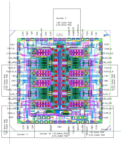
Figure 1.1: Diagram of the version 1 RMPI chip

are still crucial, with increasing attention on the GPGPU and on minimal-communication distributed computing.

This thesis brings together all of these advances and presents a state-of-the art system that bypasses a current barrier in ADC technology. The actual physical system is a receiver/ADC called the “Random Modulator Pre-Integrator” (RMPI); Figure 1.1 shows a layout of the actual integrated circuit. The general concept of the RMPI is not original to this thesis (see [SOS+_{05, KLW}+_06,

LKD+_{07, TLD}+_{10]), but it is one of the world’s first working hardware devices to be built based on}

the compressed sensing paradigm. In designing the system, numerous engineering and mathematical problems were overcome, and we hope that the results presented in this thesis will be of use to others in the field.

The second component of the system is the signal-processing back-end, which involves many steps, but the heart of the recovery is solving an optimization program. This key computation is “just” a linear program (LP), or a second-order cone program (SOCP) for fancier variants, but we will show why existing algorithms are inadequate to deal with the large quantities of data, and how our proposed algorithms make the computation tractable.

(15)

×

=

_×

=

Figure 1.2: Democracy/incoherence in measurements. Pictoral representation of linear measurements Ax = b. Historically, good operatorsAwere square and assumed to be easily invertible, such as the identity Ior Fourier matrixF. Forundersampling, choosingAto be a partial identity matrix is bad, and recovery depends on luck. For sparse signals, it turns out that we can recover all of them if measurements are sufficiently global and incoherent. We informally refer to this idea as “democracy”: each measurement provides the same amount of information as every other measurement, so there is no one special measurement without which reconstruction is impossible.

without treating the optimization problems in detail.

Chapter 3 presents an optimization algorithm “NESTA” that efficiently solves the signal-processing optimization problem for the RMPI. Chapter 4 presents an alternative optimization algorithm “TFOCS” that has some additional attractive features and is applicable to diverse problems.

The emphasis of this thesis is on the RMPI section, since this has not yet been published. The solvers (NESTA and TFOCS) have been previously described in publications [BBC11, BCG10a]. Chapters 3 and 4 are based on these publications, but contain some new material (see the chapter introductions for an overview of what is new). These chapters were written with co-authors, named in the chapter introductions.

The rest of this introduction presents some background material. The theory of compressed sensing is not discussed in much detail since there are already several excellent review articles and monographs [Can06, CW08, Bar07, FR11]; see also the resources at [RU]. Instead, we exploit the unconstrained nature of this thesis to elaborate a little on the history of some ideas that contributed to our current understanding of`1 processing, since it is rare that current literature has the luxury

of going into background.

What compressed sensing is. A brief overview of the theoretical results is reserved for_§1.2.4; we first mention the main ideas in an intuitive style. Compressed sensing (CS) addresses the situation in which there is an unknown mathematical object of interest that lies in a large ambient space, but because of prior information, the information content of the signal is less than the dimension of the space. The prior information need not be interpreted in the Bayesian sense; a more appropriate interpretation is that the signal is “compressible”.

An implication of the premise that the signal is compressible is that sampling can be performed at the “information rate”, or only marginally faster. This generally means that under-sampling is possible. As always, more samples improve the performance in the presence of noise.

(16)

mea-surement of a signal should give some global information; see Figure 1.2 for a depiction. This comes at a price: when all the measurements are combined, the reconstruction algorithm is non-linear. In fact, CS theory says that the most efficient measurements look like a random sum, regardless of the reconstruction algorithm or specific signal. Think of the Voyager 1 spacecraft taking compressed measurements and sending them back to Earth; such measurements would allow modern techniques to extract as much information as possible, even using techniques such as wavelet analysis which did not exist at the time of Voyager’s launch.

TheWired Magazine article failed to convey to its readers the importance of incoherence, hence the skepticism. To the readers, it seems as though subsampling drops information. But with incoherent measurements, every measurement gives a little bit of information, so the aberration tumor is measured, just not directly. However, compressed sensing does not give “something for nothing”. In the case of noisy measurements, it is always helpful to take more measurements since this reduces the effect of the noise, and so under-sampling will always perform worse than exact- or over-sampling (assuming the same post-processing techniques).

What compressed sensing is not. Because compressed sensing deals with sparsity and com-pressibility, it is related to many other fields, such as sparse approximation, classic problems in image and signal processing such as denoising and deconvolution, dictionary learning, computational har-monic analysis, etc. In brief, these fields are related to the first ingredients of compressed sensing: sparsity and compressibility. But since they do not fundamentally involve incoherent measurements, they are distinct fields.

The architecture proposed in Chapter 2 is a pure compressed sensing architecture, because funda-mental to its operation is the fact that measurements are incoherent. The optimization algorithms proposed in Chapters 3 and 4 are not limited to compressed sensing; they solve a wide class of problems which include CS problems, but also include problems from sparse approximation, ma-chine learning, etc. In particular, they solve so-called`1minimization problems, which have a broad

applicability.

Perhaps one of the biggest impacts of CS is that it has spurred research in related fields, with the idea of exploiting prior knowledge. Yet the impact on hardware devices is much more limited: even though compressed sensing theory is about 7 years old and is quite well understood, there are very few pure compressed sensing applications. A few novel schemes are discussed in_§1.1.

1.1 Applications

(17)

case. As mentioned earlier, only true CS devices are mentioned, and thus we consider only hardware that takes incoherent measurements.

• Optical and near-optical imaging. The iconic “single pixel camera” developed at Rice University [WLD+_{06] is the best known compressed sensing device; it was singled out in 2007}

as one of the top 10 emerging technologies by MIT Technology Review [Mag07]. The idea behind the camera is to trade spatial resolution for temporal resolution; for frequencies such as infrared, where each pixel is extremely expensive, this is a smart trade off. The camera uses a single pixel, but it takes many measurements over time. Each measurement needs to be different and also encode the entire scene; this is achieved by placing a micro-mirror array in front of a conventional optical lens system. The array is a grid of pixel-like mirrors called a digital micro-mirror device (DMD); each micro-mirror can be oriented so as to reflect light toward the single receiving pixel, or in some other direction. The effect is that of a binary mask.

This is similar to the ideas used in coded aperture imaging in astronomy since the 1960s, except that due to sub-sampling, direct inversion is no longer possible. Coded aperture imaging uses a mask that is spatially moved in order to acquire a full set of data. Similar to radio interferometry, coded aperture is used as a means to increase spatial resolution, since radio telescopes’ antenna have limited spatial resolution.

Overall, these CS-based optical devices seem promising, and InViewCorp has recently mobi-lized to commercialize such a system. Similar ideas can also be applied to microscopy [WCW+_09],

where again DMDs are used to reduce the number of raster scans needed in confocal imaging.

However, the subject is not yet closed, for there remain a few key difficulties. The first challenge is calibration. If the system can be modeled sufficiently accurately, then calibration is not an issue, but for high dynamic range acquisition, it is likely that the system will need to be characterized. Calibration at optical frequencies is challenging, since the phase is not as easy to control as in radio frequency (RF) systems.

(18)

can be resolved, but sources that have an even intensity are completely lost in the shot-noise and impossible to recover. This is currently the limiting factor in these systems.

• Medical Resonance Imaging (MRI). One of the “hot-topic” CS applications is MRI, which has seen much research, and it is also one of the first, with conference proceedings of the authors in [LDP07] going back to 2005. The work of Lustig [LDP07] has even been incorporated into the Stanford research hospital [Ell10], and current MRI manufactures are paying close attention to the field; the Siemens Corporate Research office has stayed active in the field of compressed sensing. MRI works by acquiring points in 2D or 3Dk-space (i.e., Fourier space), and conventional MRI acquires specific grids of points so that the image may be reconstructed by the inverse Radon transform. Using sparse-approximation ideas, it is possible to sub-sample this grid and solve a linear inverse problem to recover the signal. CS applies to MRI by allowing

k-space samples that are not on standard grids, and fewer samples than conventionally needed. Fewer samples leads to faster scans, which is significant since scans are performed on living, moving, people. However, the true potential of CS for MRI is that it might allow for non-standard types of measurements or certain types of systematic errors, such as non-linearities in the magnetic field, or weaker magnetic fields. To our knowledge, these types of breakthroughs have not yet happened.

• Microarray sequencing. Microarrays are used commonly in biology to identify specimens, using fluorescent tags to identify where samples bind; most samples have only a few active parts, thus using ideas from CS and group testing suggest that it is possible to take many fewer measurements and still accurately infer which specimens are present. Recent work in industry has suggested that this approach is useful in practice [MSS+_10].

• Seismic imaging. Because the Earth is made of discrete layers and so separated by sparse boundaries, seismic imaging has benefited from sparse recovery techniques since the 1970s. However, a true compressed-sensing-based seismic imaging system goes further and acquires images in a different fashion; for example, by changing the type of excitation signal sent by a ship or controlled explosion. Another method to apply compressed sensing is by controlling the rate and location of samples, much like the non-uniform sampler (NUS) introduced in

§1.4.1. Undersampling is a fact of life for many seismic imaging systems; the system in [HH08] proposes that undersampling should be nearly at random, like the NUS, in order to turn coherent aliases into incoherent noise. They also suggest that the undersampling should not be completely at random; instead, the maximum separation between measurements should be controlled.

(19)

0 0.5 1 1.5 2 2.5 −190

−180 −170 −160 −150 −140 −130 −120 −110

Frequency (GHz)

Power/frequency (dB/Hz)

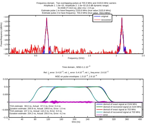
Frequency domain. Two overlapping pulses at 703.3 MHz and 2103.6 MHz carriers Amplitude 1: 1.0e−02, Amplitude 2: 1.0e−02 (0.0 dB dynamic range)

N=2048 (T=410 ns), jitter rms = 0.5 ps Estimate pulse 1 to have frequency 2103.6 MHz (true value 2103.6 MHz)

Estimate pulse 2 to have frequency 703.3 MHz (true value 703.3 MHz) original recovered

0 40 80 120 160 200 240 280 320 360 400

−0.01 −0.005 0 0.005 0.01 0.015

time (ns) Time domain., MSE=1.1⋅10−3

Rel. l2 error: 3.4⋅10 −2_{; rel. l}

∞ error: 5.4⋅10−2_{; rel. l}

∞ freq error: 2.6⋅10−2

MSE on pulse envelopes: 1.5⋅10−3_{, 2.6}_⋅₁₀−4

TOA estimate: 66.6 ns, Actual: 67.0 ns, Error: 0.4 ns Duration estimate: 200.8 ns, Actual: 199.8 ns, Error: 1.0 ns TOA estimate: 107.2 ns, Actual: 110.2 ns, Error: 3.0 ns Duration estimate: 204.2 ns, Actual: 200.0 ns, Error: 4.2 ns

[image:19.612.198.445.77.287.2]

demod of exact signal at 2104 MHz demod of recovered signal at 2104 MHz demod of exact signal at 703 MHz demod of recovered signal at 703 MHz error

Figure 1.3: Preview: beating Nyquist with the RMPI. Reconstructing two pulses from 2.5 GHz of bandwidth using only 400 MHz sampling rate in a realistic simulation with noise and non-idealities.

ease identification; for example, it may aid a satellite imaging the ground, trying to determine the type of foliage on the surface. Images are typically compressible, and hyperspectral images even more so. See the work in [WGB07] for a proposed hyperspectral imaging system that uses a binary aperture mask (similar to the single pixel camera) with a multi-pixel array.

• Radar. Much like seismic imaging, it is possible to design special radar pulses to exploit CS; for example, [HS09] proposes sending a type of chirp called an Alltop sequence to probe targets, and shows that when there are only a few targets, this allows greater resolution than traditional radar. This is distinct from the radar problems discussed in this thesis. Typical CS radar applications design an emitter and a receiver; in this thesis, we are concerned with learning pulse characteristics from a foreign object’s radar emitter, so not only is there no control over the emitted pulses, but the pulse parameters are unknowna priori.

(20)

pseudo-random matrix (a noiselet transform [CGM01]) to multiply groups of 6 images; importantly, this operation is easy to carry out in the satellite. The compressed data is sent to Earth and decompressed using`1 techniques or similar. The Herschel satellite adopted this scheme, so it

is one of the first compressed sensing hardware devices, even if the image acquisition is still conventional. For more details of CS in astronomy, see [SB10].

• Quantum physics. In quantum computing and related fields, quantum states are prepared for specific purposes, and it is important to verify that an experiment has produced the expected state. The process of verifying a quantum state is known as quantum tomography. In an

n qubit system, there aren particles but the spin of the system cannot be represented by a

n-dimensional state vector due to entanglement. Instead, the system can be represented by a

n_×nHermitian matrix. In a generic high entropy system, this matrix is rankn, but in specially prepared states, the matrix has low rank, or even rank 1. In a collaboration with quantum information physicists, this author worked on the problem of estimating the quantum state via subsampled measurements [GLF+_{10]. Measurements are taken in an incoherent fashion;}

unfortunately, the best type of measurements are difficult to enact experimentally. Feasible measurements that are slightly less optimal are also proposed. The situation is interesting for several reasons. The first reason is that there is much experimental control over which measurements are taken, and no calibration is needed. It even allows the possibility of adaptive measurements. Secondly, measurements are inherently noisy because they are samples of a quantum wave function. Each measurement is really a Bernoulli random variable, so repeated measurements are binomial random variables. Thus the noise can be made arbitrarily small at the expense of requiring more time. Furthermore, in the experimental setup, there is a time penalty for switching to a new measurement, so it is advantageous to take repeated measurements of the same quantity. These tradeoffs make for interesting future study.

• ADC (Analog-to-Digital Converters). A compressed sensing ADC device is presented in Chap-ter 2 and also in §1.4, where history and background will be presented in detail, so we defer discussion. Figure 1.3 shows the recovery of two radar pulses from a realistic simulation that included non-idealities of the circuit.

(21)

ap-0 0.1 0.2 0.3 0.4 0.5 0.6 0.7 0.8 0.9 1 0

0.1 0.2 0.3 0.4 0.5 0.6 0.7 0.8 0.9 1

N=30, d.f. = 60; obs. radius=0.29, # obs = 190 = 3.2⋅ d.f. max error is 5.6e−16 (after rotation)

Original points Observed distances Radius of observed distances Estimated points

Denver Chicago Atlanta Dallas Seattle

Denver 0 ? 591 398 ?

Chicago ? 0 218 ? 982

Atlanta 591 218 0 634 ?

Dallas 398 ? 634 0 521

[image:21.612.126.514.72.254.2]

Seattle ? 982 ? 521 0

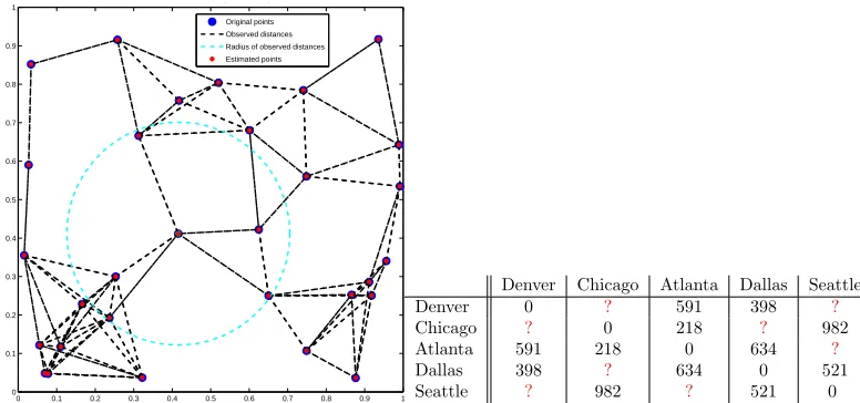
Figure 1.4: Preview: distance completion. In general, this is an NP-hard problem, but sometimes the convex relaxation is exact. The algorithm proposed in Chapter 4 can solve these minimization problems that involve matrix variables. This problem is like filling in the unknown “?” entries in the sample mileage chart on the right. The plot on the left shows a set of points for which about 29% of the pairwise distances are known (line segments represent known distances); from this, their true positions are recovered.

[image:21.612.179.468.480.571.2]

plications in many communications and network problems, and can be used to solve general statistics estimation problems. Thus our algorithms apply to almost all fields in the sciences. The algorithms can also solve certain matrix-variable problems in low-rank (and/or sparse) recovery. Such problems include matrix completion [CR09, Gro11] and various variants of robust PCA [CLMW09, MT10] (Figure 1.4). TFOCS can solve general semi-definite programs (SDP) [VB96]. Over the past 15 years, an increasing number of problems from engineering and control theory, as well as the fields mentioned above, have been cast in this framework. SDP relaxations of difficult problems such as MAX-CUT and matrix completion are also of high interest.

image 2D DCT coefficients reconstructed image

Figure 1.5: Compression. The image on the right is reconstructed from less than half the DCT coefficients of the original image on the left. It is an empirical fact that real images are usually compressible in the 2D frequency domain. JPEG uses an 8×8 2D DCT (in HSV color space) and quantizes coefficients, and has revolutionized the internet. The algorithms in Chapters 3 and 4 can be used for much more advanced image processing problems; see Figures 1.6 and 4.8.

1.1.1 Problems of interest

(22)

[image:22.612.168.483.78.234.2]

Figure 1.6: Preview: image denoising with TFOCS. For full details, see Figure 4.8. The image on the right is a denoised version of the noisy image on the left.

inverse problem, we seek an estimate ˆxof a true signalx0 given (possibly noisy) measurements of

the formulation

b=Ax0+z, x∈Rn, b∈Rm, A∈Rm×n (1.1.1)

where z is a noise vector (usually stochastic). On occasion we allow complex numbers, and this will be explicitly stated. The model b =A(x+ ˜z) also arises, which is equivalent to (1.1.1) if we set z =Az˜. Thelinearity of the problem means that A is a linear operator, and since this thesis only considers finite dimensional problems,Ais a matrix. Estimates for ˆxare not necessarily linear functions ofA andb.

This thesis is concerned with the under-determined case, m < n, but the algorithms are also useful in the ill-conditioned case wherem=nbutAis either singular or has large condition number. The focus is not on them=ncase, and it is assumed thatAhas full column rank unless otherwise stated. Recovering an arbitrary vector xfrom a given A and b is then ill-posed because there are infinitely many solutions to this under-determined equation.

Consider temporarily a problem in whichm > n, so the situation is over-determined. A standard approach (ifzis Gaussian, this is the maximum likelihood estimator) is to set ˆx= argminxkAx−bk22,

which is the famous “least-squares” estimator made popular by Gauss. This can be written in closed form as ˆx=A†_b_where_A†_{= (}_AT_A₎−1_A_{is the Moore-Penrose pseudo-inverse of}_A_{. In the case that}_A

is ill-conditioned, a classical technique is to regularize the problem (known as Tikhonov regularization or ridge regression):

ˆ

xγ = argmin x k

Ax+b_k2

2+γkxk22= (ATA+γ2I)−1ATb. (1.1.2)

(23)

on the choice ofγ. If it is assumed that the signalx0comes from a normal distribution with mean 0

and varianceσ2_I_{(which we will write as}_x

0∼ N(0, σ2I)) andz∼ N(0,I), then this is the maximum

a posteriori(MAP) estimator if we choose γ=σ. In some contexts it may be possible to chooseγ

via cross-validation.

The `2 norm used in (1.1.2) is part of the class of `p norms, defined on a vector x as kxkp =

(P

i|xi|p)1/p; so kxk1 =Pi|x|is just the sum of the absolute values. The `0 quasi-norm is not a

norm: it just measures the number of non-zero entries of a vector.

We use Tikhonov regularization to motivate our first problem of interest, called the LASSO [Tib96] (Least Absolute Shrinkage and Selection Operator):

ˆ

x= argmin

x

1

2kAx−bk

2

2+λkxk1. (1.1.3)

This is quite similar in form to Tikhonov regularization. From a Bayesian perspective, (1.1.3) is the MAP estimator ifxhas a Laplacian prior andz is i.i.d. Gaussian. At the solution ˆx, the first-order stationary condition [BV04] gives

AT(b₋Ax)_∈λ∂_kx_k1

where ∂f is the sub-differential of f [Roc70] (that is, the set of all sub-gradients). In particular, the absolute value of every entry of ∂_kx_k1 is bounded by 1. If the original signal x0 were to be a

solution, then this gives the necessary condition that_kAT_z

k∞≤λ. Whenzis a general stochastic

vector, it is not expected that ˆx is exactly x0, but it turns out that λ≈ kATzk∞ is a reasonable

value for the parameter. Ifz_{∼ N}(0, σ2_I_{), then with high probability}

kAT_z

k∞≤2plog(n).

The key difference between the LASSO and Tikhonov regularization is that the `1 norm has a

sharp discontinuity at 0; see Figure 1.7. A closely related problem is the following:

minimize

x kAx−bk

2

2 such that kxk1≤τ. (1.1.4)

Confusingly, this is the version suggested by Tibshirani in his original LASSO paper [Tib96] so it also goes by the name “LASSO”. To keep the variants clear, we will stick with theλorτparameters, and refer to the first problem as the “unconstrained LASSO”. The unconstrained LASSO has seen much more attention in the literature than the`1 constrained LASSO.

Another variant is known as basis pursuit (BP) [CDS98], which is the linear program (LP):

minimize

(24)

−1 −0.8 −0.6 −0.4 −0.2 0 0.2 0.4 0.6 0.8 1 0 0.1 0.2 0.3 0.4 0.5 0.6 0.7 0.8 0.9 1

f(x) = |x| dual smoothed f(x) primal smoothed f(x)

(a) The absolute value function (blue), a primal smoothed version known as the Huber function which will be used in Chapter 3, and a dual smoothed version which will be used in Chapter 4

−1 −0.8 −0.6 −0.4 −0.2 0 0.2 0.4 0.6 0.8 1 −1 −0.8 −0.6 −0.4 −0.2 0 0.2 0.4 0.6 0.8

1 µµ = 0.1 = 1.0

µ = 2.0

(b) Contours of the dual smoothed ab-solute value function, for various levels of smoothing

−1 −0.8 −0.6 −0.4 −0.2 0 0.2 0.4 0.6 0.8 1 −1 −0.8 −0.6 −0.4 −0.2 0 0.2 0.4 0.6 0.8

1 µµ = 0.01 = 0.20

µ = 0.50

(c) Contours of the Huber function for various levels of smoothing

Figure 1.7: The `1 norm promotes sparsity because of the kink at 0. Any function which is quadratic near zero

(e.g., least-squares norm, or the Huber function [Hub64]) does not promote sparsity because of the “diminishing returns” in pushing a coefficient to zero. The dual-smoothed version keeps this feature. Unfortunately, the non-smoothness of`1also makes it difficult to work with; only the Huber function has a continuous derivative. See also

Figure 4.1

which always has the same value as its dual problem

maximize

ν b

T_ν _{such that}

kATνk∞≤1.

This is mainly used whenz= 0. For noisy cases, we turn to basis pursuit denoising (denoted BPDN orBPε), which is a second-order cone program (SOCP) [BV04]:

minimize

x kxk1 such that kAx−bk2≤ε (1.1.6)

and its dual

minimize

ν kνk2−b

T_ν _{such that}

kAT_ν

k∞≤ε.

This dual problem has the same value as the primal problem whenA has full row-rank andε >0 (see the Slater conditions [BV04]). BPDN is sometimes referred to as the LASSO as well.

BPDN will be the focus of the optimization algorithms introduced in later chapters. A basic result of convex optimization [Roc70, BNO03] is that unconstrained LASSO, the `1 constrained

LASSO, and BPDN are all equivalent for some values ofε, τ, andλ(as long as these are all non-zero and finite). That is, givenε, there is someλ(ε) such that the unconstrained LASSO estimator is the same as the BPDN estimator. In general, calculatingλ(ε) is not easy, and requires at least as much computation as solving the estimation problem; for example, to calculateε(λ), we setε=_kAxˆλ−bk2

(25)

The value ofεis typically chosen by ε_'Ekzk2. If the entries ofz are independent and have a

finite second moment (and zero first-moment), this is just the square root of the sum of the variances. Methods for estimating variances, using the sample variance or a robust statistic like the median absolute deviation, are well-understood, so it is quite reasonable to assume that a reasonable value of ε is known. In practice, some researchers may prefer to estimate εrather than λ; this was the motivation behind NESTA’s development.

The final canonical problem we discuss is the Dantzig selector [CT07a], which motivated the development of the TFOCS algorithm. The Dantzig selector is the solution to

minimize

x kxk1 such that kA T₍_Ax

−b)_k∞≤δ. (1.1.7)

The parameter δ should be about the same as the parameter λ from the unconstrained LASSO. The Dantzig selector is used for the same types of problems as BPDN, and enjoys similar theoretical properties. Indeed, the differences between the two was the subject of much discussion in the Annals of Statistics (see [EHT07, CT07b] and related papers in the same issue).

Lastly, we present two variants of BPDN that are useful when a signal x0 is compressible in

some basis or dictionary Ψ; these variants can also be applied to the LASSO and Dantzig formu-lations. Supposex0 = Ψα0 (this is useful whenα0is sparse or has decaying coefficients), and take

measurementsb = Φx0+z = ΦΨα0+z. There are two ways to use BPDN. The first is known as

“synthesis”:

minimize

α kαk1 such that kAα−bk2≤ε, A,ΦΨ (1.1.8)

and the second is “analysis”:

minimize

x kΨ T_x

k1 such that kΦx−bk2≤ε. (1.1.9)

Since we are often interested in solving the analysis problem, it is convenient to allow BPDN (and the other variants) to use weighted `1 norms; we often write W for the weighting matrix,

e.g.,W = ΨT_{. The differences between synthesis and analysis are discussed in}

§2.7.2.1,_§3.6.1, and

§4.7.5.

1.2 Historical development

(26)

1.2.1 Classical signal processing

We start with the following fundamental theorem.

Theorem 1.2.1 (Shannon-Nyquist-Whittaker, this form modified from [Mal08]). Let x(t) be a band-limited signal with frequencies inside the band[−B, B](in Hz). Then

x(t) =

∞

X

n=−∞

x(n∆T)φs(t−n∆T)

where fs ,2B is the “Nyquist rate” or “Nyquist frequency”, ∆T ,1/fs, and φs = sin(2₂_πfπf_sst) is a scaled sinc function.

The theorem is obvious using the machinery of the inverse Fourier transform and convolutions, and noting that the Fourier transform of a sinc is a boxcar function; this may explain why it was discovered independently by several people in the first half of the 20th century. In [ME09a], it is referred to as the WKS theorem, where the K stands for Kotel´nikov.

In plain language, Theorem 1.2.1 states that if a signal has bandwidth B, then it is completely specified by sampling at ratefs= 2B. For an arbitrary bandlimited signal, this sampling rate is also

necessary, otherwise aliasing occurs and the original signal cannot be reconstructed from the samples. Sampling theorems such as these are important since most algorithms manipulate digitized signals, and digitizing an analog signal requires sampling. The bandlimited assumption is quite natural since most receivers and emitters have finite bandwidths (or more accurately, nearly finite bandwidths: at very high frequencies, signals are attenuated so much that they can be neglected).

Suppose now that a bandlimited signal only has small spectral occupancy. If these are in a few continuous regions, and are known, then down-conversion tricks (see§1.3) show that the sampling rate only needs to be at twice the amount of occupied bandwidth. A more precise, general and robust result is due to Landau [Lan67] from the 1960s. In the following, _F denotes the Fourier transform.

Theorem 1.2.2 (Landau sampling theorem; this form modified from [ME09a]). Define

BΩ={x(t)∈L2(R)| supp(Fx(f))⊂Ω}.

A set of time samplesR={rn} is a sampling set forBΩ if the sequence of samples xR[n] =x(rn) is stable; stability means_∃α >0, β <∞ such that

(27)

Then a necessary condition forR to be a sampling set for_BΩ is

D−(R), lim

t→∞yinf∈R

|R∩[y, y+t]|

t >|Ω|

where_{| · |} is the Lebesgue measure. The termD− _{is known as the lower Beurling density.}

For example, ifRtakes uniform samples with spacing ∆T, thenD−_{= 1}_/_∆_T _{which is the average}

sampling density. If in addition Ω = [₋B, B], then the theorem requires 1/∆T >2B, which is just the Shannon-Nyquist theorem.

Note an interesting consequence of the theorem: ifx(t) = sin(2πf t) is a pure tone, then|Ω|= 0 so the theorem does not provide a minimal necessary sampling rate to recover this signal. In fact, any periodic signal has a zero measure frequency support, and hence the theorem provides no bound. For practical recovery from such a model, and sampling at the minimal rate, it is necessary to know Ω. An example of a related compressed sensing result is due to [ME09a], which, to paraphrase, says that if the frequency support Ω of X is unknown but _|Ω_| is bounded and it is known that Ω_⊂[₋B, B], then a necessary condition for a sampling set that stably recovers all signals in this model is that its lower Beurling density must be twice the value it would have been had Ω been a fixed, known set.

1.2.2 Estimation and the rise of alternatives to least-squares

Least-squares is the quintessential linear estimation technique; the ordinary least-squares (OLS) solution to an overdetermined system minxkAx−bk2 is ˆxOLS =A†b which is linear inb. Starting

with at least Gauss, the nice properties of least-squares estimation (smoothness, convexity, closed-form expressions) have been much touted.

Particularly because of the rise of computers in the 20th century, there have been an increas-ing number of alternatives to linear methods. These alternatives have accumulated gradually but steadily: Dantzig’s simplex algorithm in the ’40s, message passing and belief propagation used for decoding (Viterbi’s algorithm in the ’60s), and graphical models used for inference in the past two decades, to name just a few. Linear estimation is certainly still a cornerstone technique and has produced successes like the Kalman filter. Below is a brief and partial history of some ideas that form a foundation for modern compressed sensing. Most of these are related to processing sparse signals and using`1techniques; the idea of using incoherent measurements has much less precedent,

with perhaps the exception of coded aperture receivers.

In 1965, Logan’s dissertation [Log65] proved a result now known as “Logan’s phenomenon”: if a continuous-time band-limited signal x(t) is corrupted by noise z and the noise has bounded L1

norm and has a very sparse time support (but the support is unknown), then finding the minimalL1

(28)

because it is independent of the magnitude of the error.

The discrete version of this result, using the`1 norm, was empirically demonstrated by Santosa

and Symes [SS86] in 1986, and proved in [DS89]. The work of [SS86] proved that recovery of a

k-sparse vector from just m Fourier measurements was possible if m _≥ (1₋1/(2k))n, using the unconstrained LASSO formulation (they also note the pessimistic nature of this bound). Even by 1986, the fact that “it is possible to construct a sparse spike train from part of its spectrum using the minimum`1criterion” was “well-known (and believed)” [SS86].

The 1989 article by Donoho and Stark [DS89] extended Santosa and Symes’ results by proving a more general new type of uncertainty principle (see also [DL92]). The classical time-frequency uncertainty principle says that a signal cannot have small support in both time and frequency. The [DS89] result extended this result by relaxing the restriction that a signal’s support be on intervals. To be concrete, let xbe a discrete signal of lengthnwith discrete Fourier transformX. Donoho and Stark prove

kxk0kXk0≥n

and hence, kxk0+kXk0≥2√n

. (1.2.1)

Intuitively, the result says that there are not many discrete signals that are sparse in both time and frequency. Thus, if a signal happens to be sparse in both time and frequency, it has no “neighboring” signals, and for this reason it is easy to recover. The multiplicative inequality is sharp, because if

n = d2_{, then a Dirac comb of spacing} _d _has _k_x_k

0 = kXk0 = d; this example is also sharp for

the additive identity (the additive identity follows from the multiplicative one by the arithmetic-geometric mean inequality). Another example is whenxis a single Fourier element, in which case

kx_k0=nandkXk0= 1, so the multiplicative inequality is sharp but the additive inequality is not.

It turns out the additive inequality is only sharp in cases such as n=d2_{; the situation when}_n _is

prime is quite different [Tao05].

[DS89] also reports numerical experiments suggesting that much stronger results are possible if the sparsity is “scattered” in a random way, so it is clear that the authors had some insight into what was achievable; their official bound on measurements was the same as Santosa and Symes. It is worth mentioning that their numerical experiments went only as large asn= 256, and it is not easy to distinguishO(n),O(√n), andO(logn) growth from experiments with justn={64,128,256}.

This theory in the late 1980s built on empirical work from the previous 15 years, as different scientific communities were using `1 minimization and/or sparsity. The work in [CM73] in 1973

argues that the geophysics community should consider `1 regularized problems for the sake of

ro-bustness to outliers, using the mean and median estimators as examples. They also argue that `1

(29)

examples of using sparsity in first- and second-differences; this was further explored in the highly influential total-variation (TV) minimization paper in 1992 [ROF92].

Similar works in geophysics, such as [TBM79], cite `1 studies going back to 1964. Incremental

results continued in geophysics, exemplified by [OSK94] in 1994 which cites numerous `1 results

from the 1980s (but appears to be unaware of [SS86, DS89]). Many of these works proposed special algorithms to avoid recasting the problem as a linear program (LP).

In radio astronomy, the CLEAN algorithm [H¨og74], introduced around 1971, exploits sparsity of radio sources and is similar to a matching pursuit algorithm [MZ93] as shown by [WJP+_{09], though}

it is not equivalent to`1 minimization (indeed, the first analysis of CLEAN [Sch78] compares it to `2 minimization). Its idea of exploiting sparsity and post-processing has been extremely useful in

astronomy; to quote from [Cor09], “The impact of CLEAN on radio astronomy has been immense. First, there is the accumulated science from the telescopes that have used CLEAN—GBI, MERLIN, WSRT, VLA, VLBI, etc. ... Second, by showing what could be achieved with some postprocessing, CLEAN has encouraged a wave of innovation in synthesis processing that continues to this day.”

The article [PC79] introduces the authors’ algorithms from 1975 to the application of estimating the transfer function of an unknown medium using ultrasound pulses, and exploits sparsity in the number of layers in most mediums. The algorithm they propose is similar to alternating projections between the time domain (which is sparse; this set is not convex) and the frequency domain (where it is assumed that reliable data exists in some band). The 1982 article [ME82] discusses an applica-tion of `1 minimization for improving diffraction-limited images, and also suggests its use in video

compression.

A noticeable similarity in all these works is that they almost exclusively work with deconvolution, and hence operate in the Fourier and time/spatial domains.

1.2.3 Leading up to compressed sensing

Another key milestone in the work preceding compressed sensing was a paper by Donoho and Huo in 1999 [DH01], and was followed by several papers in the next five years, including [DE03, EB02, GN03, Tro04, DET06, Tro06]. These results concern sparse approximation: suppose a signalx_∈Cn

can be represented as x= Ψαwhere Ψ = (I,F) contains “spikes and sines” (F is the DFT). Since Ψ is rectangular, there are infinitely manyαwhich satisfy this. The result of [DH01] is that if there is somekα0k0<1₂√nandx= Φα0, then`1 minimization

min

α kαk1 such that x= Φα

will returnα0. Similar results hold for solving by Orthogonal Matching Pursuit (OMP; see§1.5) [Tro04].

(30)

The result means that a signal α_∈C2n of lengthN = 2nwhich isksparse, withk < 12

√_n_{, can}

be recovered fromm=n entries. In terms of the dimensionN and measurements m, the sparsity must obey k < _√1

2

m

√

N. This

√

N sparsity may not seem very sparse to readers with knowledge of recent results, who might expect that sparsity can grow with rate k _' m

logN, which only weakly

depends onN. But as proved in [DH01], these results are sharp. Other than special cases (such as

nprime; see [Tao05]), there are counter examples showing that better bounds cannot be obtained, such as with the Dirac comb. So how does compressed sensing improve these bounds? The key difference is that compressed sensing bounds typically do not hold for all measurement matrices, but rather hold with overwhelming probability1 _{or with high probability}2_.

1.2.4 Compressed Sensing

This section gives a brief review of basic CS theory; for more details, the short review article [CW08] is recommended.

Let a signal x(t) =Pn

i=1αiψi(t) where Ψ is the matrix with columns ψi. We deal mainly with

discrete, finite-length samples, sox_∈Rn, and Ψ is an×nmatrix, typically chosen to be orthogonal.

For example, the signalxmight just be a sparse vector, so then Ψ can be the identity matrix I. Let Φ be another orthogonaln_×nmatrix; we will eventually subsample this to create them_×n

“sampling matrix”; outside of the introduction, it is always assumed that Φ ism_×nwith m < n, and except for the NESTA algorithm in Chapter 3, the rows of Φ will not need to be orthogonal. Since Φ and Ψ are both orthogonal, and therefore invertible (and well-conditioned), it is possible to recoverx(or equivalently,α) from samples

b= Φx= ΦΨα, or b=Aα, A,ΦΨ.

So far, this is not remarkable, and there is no benefit to doing so (even in the noisy case, since Gaussian white noise is unchanged under orthogonal transformations).

The remarkable results from compressed sensing say that if α is sparse (we typically usek to denote the sparsity, and say that αis “k-sparse”) and Φ and Ψ are incoherent, then it suffices to only take a little more thankrows of the Φ matrix in order to stably reconstructx.

Define thecoherence of Ψ and Φ to be

1_≤µ(Φ,Ψ),√n max

1≤k,j≤n|hψk, φji| ≤

√

n. (1.2.2)

The two ortho-bases are “incoherent” when µ_'1 or has a weak-dependence on the dimension n.

1_{Used here, this is a technical term (see [Tao11]); if a statement or event}_E

n depends onn, thenEnholdswith overwhelming probability if ∀α >0 we have∀n,P(En)≥ 1−cαn−α where cα is a constant independent ofn; in

compressed sensing,nis the dimension of the signal.

2_{Similarly, we say}_E

(31)

Complete coherence, µ=√n, is obtained if, for example, Ψ = Φ. Maximal incoherence,µ= 1, is obtained for Ψ =F, the Fourier basis, and Φ =I, the identity. One remarkable fact is that for any

fixed basis Ψ, if Φ is chosen from the general orthogonal ensemble (GOE), the coherence of Φ and Ψ is

√_{2 log}_n_{with high probability. Thus random matrices Φ are universally good measurement matrices.}

Intuitively, we want low coherence so that each row of Φ takes an equal amount of information about the signal. If Φ and Ψ are very coherent, then each row of Φ only tells us how much of one particular basis elementψiis present in the signal, and thus we would need all nmeasurements, since leaving

out theith measurements is taking the very risky gamble thatαi= 0. See Figure 1.2 on page 4 for

a graphical depiction.

An early result [CR07a] is that if

m_≥Cµ2(Φ,Ψ)klogn

then if α is k-sparse and Φm is Φ restricted to m rows chosen uniformly at random, then with

overwhelming probability, the measurements b = Φmx are sufficient to tractably recover x. The

recovery is tractable because it can be done by solving basis pursuit (1.1.5), which can be solved in polynomial time. Here,Cis a constant that is independent ofkandn.

Very recent results [CP10a] have extended this, which we briefly paraphrase. For simplicity, let

A incorporate both Φ and Ψ,A= ΦΨ. Write the rows ofAas aT

i, and assume each row is drawn

iid from some probability distributionP, and that each row has zero mean and identity covariance matrix (so in particular, all the entries ai,j of A are uncorrelated, and furthermore entries from

different rows are independent). Define the self-coherence to be the smallest numberµs such that

for all rowsai,3

max

1≤j≤n|ai(j)|

2

≤µs. (1.2.3)

If P is a sub-Gaussian distribution, then µ = clogn for some c independent of n, and if P is sub-exponential,µ=clog2n.

From now on we’ll assumexis the sparse object, e.g.,x=α. The following theorem differs from other compressed sensing results in that we assume xis a fixed k-sparse vector. This is a stronger assumption than before because for any given realization of a sampling matrixA, we can no longer pick an adversarial signal (and one might argue that since adversarial signals rarely arise in practice, this stronger assumption is palatable).

Theorem 1.2.3 (due to [CP10a]). Let x be a fixed k-sparse vector, and take m measurements

b = Ax. If m ≥ (1 +β)Cµsklogn then with probability 1−5/n−e−β, basis pursuit (1.1.5) will recover x.

(32)

This can be extended to cover compressible signals and noisy measurements. Letxk denote the

bestk-term approximation tox; in loose terms, we sayxis compressible if there is a small ksuch that_kx₋xkk2is small. In particular, ifxisk-sparse, thenx=xk. We present a simplified theorem

below:

Theorem 1.2.4(due to [CP10a]). Letx_∈Rn be arbitrary; in particular, it need not be sparse. Let y=Ax+z wherez_{∼ N}(0, σ2₎_{, and define} _λ_{= 10}_σ√_log_n_{. Then if}

m_≥(1 +β)Cµsklogn

then with probability at least1−6/n−6e−β, the LASSO (1.1.3)will recover an estimatexˆsatisfying

kxˆ₋x_k2≤C˜(1 + log2n) k

x₋xkk1

√

k +σ

r

klogn

m

!

.

Identical results hold for the Dantzig selector (1.1.7).

To make these results meaningful, we compare to an “oracle”. Similarly to how an unbiased estimator’s performance can be compared to the optimal performance given by the Cram´er–Rao bound, comparing with an oracle gives an idea of how close this performance is to the optimal performance. Consider recovery of ak-sparse vectorxgiven noisy observationsy=x+σz, wherez

is any noise vector with independent entries and unit variances. Suppose an oracle whispers in your ear that the nonzero entries ofxare precisely the firstk. Then a quite reasonable strategy (though not optimal in terms of mean-square error, as Willard James and Charles Stein famously showed) is to take ˆxi=yi fori≤k and ˆxi = 0 otherwise; in fact, with this information, we only need to take

kmeasurements. The expected error isEkxˆ−xk2=kσ2, and this is referred to as the oracle error.

The oracle takeskmeasurements and the error iskσ2_{. The above theorem says that without the}

benefit of knowing a priori which entries are nonzero, then if we take slightly more measurements (by a factor of about logn), we can do almost as well, with an error that is worse by a factor of about log5n. Theorem 1.2.6 will improve this to a constant factor, and in Chapter 2 we show empirically that this factor is about 3.

For completeness, we cover what is now the de facto “standard model” of compressed sensing, which relies on a tool called the RIP:

Definition 1.2.5 (RIP (Restricted Isometry Property)). The restricted isometry constant δk of orderk for a matrix Ais the smallest number such that

(1−δk)kxk22≤ kAxk22≤(1 +δk)kxk22

(33)

For example, ifAis an orthogonal matrix, thenAis an isometry, andδk = 0 for anyk, which is

the best possible constant. IfA ism_×n, then it has a non-trivial nullspace, soδk ≥1 fork≥m,

but it is still possible for δk <1 for k < m. In general, adding rows to a matrix A will improve

(i.e., decrease) its RIP constant. The literature often refers informally to a “matrix having the RIP” whenever that class of matrices satisfies δγk 1 with high probability whenever m ' klog(n) ,

whereγ is typically 2 or 3. There are many variations of results using the RIP, but we show one of the most compact results.

Theorem 1.2.6(due to [Can08]). Letδ2k <

√

2₋1andb=Ax+z for any (possibly deterministic)

z, with_kzk2≤ε. Then basis pursuit denoising (1.1.6) with thisεgives an estimator xˆ satisfying

kxˆ₋x_{k ≤}C0k

x₋xkk1

√

k +C1ε

for some constants C0 and C1 (which are not unreasonably large).

The theorem is deterministic, but unfortunately, there are few deterministic matrices which have small RIP constants. For a fixed number of rows m, random matrices have the best known RIP constants (although these bounds are not deterministic, and hence there is a nonzero chance of failure). The boundδ2k <

√

2₋1 can be slightly improved, but this has little qualitative significance to our study here.

There are different bounds for random matrices, but we present here a paraphrase of an elegant result that sums up the general idea:

Theorem 1.2.7(due to [BDDW08]). Let the entries of them_×nmatrixAbe drawn i.i.d. according to either a zero-mean Gaussian or_{+1,−1} Bernoulli distribution, and scaled so the expected value of each column is1. For anykandδ, with overwhelming probability (which depends onδ) the matrix

A will satisfyδk(A)≤δ as long as

m≥Cklog(n/k)

for some constant C independent ofn(but dependent on δ).

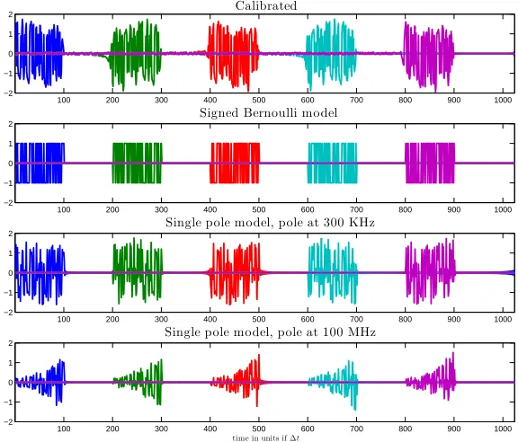
Note that there is a qualitative difference between the _{+1,₋1_} Bernoulli matrices (also known as signed Bernoulli, or Rademacher) and the{0,1} Bernoulli matrices in their compressed sensing performance; the simple shift makes a big difference. In fact, {0,1} matrices do not obey the RIP unless m scales with either k2 _or _n _{(as opposed to} _k_log_n_{) [Cha08]. This does not mean that}

(34)

Figure 1.8: Group testing. SupposeN soldiers are tested for a disease using a sensitive but expensive blood test; if blood from different soldiers is grouped together, the test is sensitive enough to declare a “positive” if any of the contributed blood samples were positive. Ifksoldiers are infected, how many measurementsM are necessary? If

kis large, thenM =N is the best we can do. Ifk= 1 (andkis knowna priori), thenM= log2(N) is possible

(with or without adaptive measurements). The key idea is to take global measurements and then use reasoning. In this pictorial example, soldier # 45 tests positive, and 45 is 101101 in binary, so using the binary tests depicted by the gray shading, and assumingk= 1, we can deduce that this is the infected soldier. Each row represents one test, which involves the columns that are gray. See [GS06a] for more info. This was first proposed in the 1940s by two economists helping the military screen draftees for syphilis; their proposal was to group together the blood of five men and apply the test. Since few men were likely to have syphilis, this saves tests on average. The test was never put into practice, in part because the test was barely sensitive enough to detect a positive hit from diluted blood. The subject was revived again in the late 1950s.

Another useful result of CS is that random rows of a discrete Fourier matrix also work well for sampling when the signal is sparse. This is significant since the fast Fourier transform allows one to compute measurements faster than simply taking a matrix-vector product. The number of required measurements is similar to that of the Gaussian ensemble case, except the log(n) factor is log5(n); this bound may be lowered in the future, so it is not necessarily indicative that Fourier matrices are inferior to Gaussian matrices in practice.

To summarize the intuition behind compressed sensing: if a signal has a sparse representation, then typically only_O(klogn) measurements are necessary (this is an intuitive number: for each of theknonzeros, we need some constant number of measurements to encode the amplitude, and logn

number of measurements to encode the location of the entry).

The other intuition is that for a noisy signal, the undersampling hurts us, but only by an amount proportional tom/n. This is a fundamental limitation: to accurately estimate a quantity given noisy measurements (say, estimate the population mean given the sample mean), it is always beneficial to take more measurements.

Our final remark is that because random sensing matrices have good properties, CS tells us they are universal encoders. Furthermore, the measurements are not adaptive. Clearly, well-chosen adaptive measurements are not detrimental, but perhaps they are not as beneficial as one might expect. For example, consider the case of group testing [GS06a, DH93] depicted in Figure 1.8, with

n samples and k samples that test “positive”. We wish to find the k positives. If k = 1 and

k is known, then one obvious solution is an adaptive binary tree scheme (aka bisection method) which will take log2n measurements. But a non-adaptive scheme that groups the measurements

according to their binary representation also takes log2nmeasurements, so there is no advantage to

(35)

Alternatives to RIP. The RIP is a convenient tool, but so far it has not proven to be the perfect tool to analyze deterministic matrices. Most undesirably, it is generally NP-hard to check if the RIP holds for a specific matrix. Furthermore, the RIP is not a necessary condition. It is clearly a useful tool, but because of the importance of CS, there has been work on alternatives. We mention just a few of these alternatives here, in addition to the coherence property which was already discussed.

The work in [BGI+_{08] introduces a simple extension of the RIP to the so-called RIP-p, and in}

particular the RIP-1. The RIP-p is stated as the RIP is, except using`pnorms instead of the`2norm;

thus RIP-2 is the standard RIP. The RIP-1 is particularly useful for expander graphs [JXHC09] and other sparse encoding matrices. Another extension of the RIP is model-based RIP [BCDH10] which concerns allxrestricted to a specific model; if the model is the set of k-sparse signals, then this is just the usual RIP. A variant on this is the restricted-amplification property [BCDH10].

Another approach is that taken by Donoho in his original paper [Don06]; see [DT10] for an overview. Results are proven using combinatorial geometry, and using results on Gel’fand n-widths. The approach in [XH11] is a simple nullspace condition that is both necessary and sufficient, and uses Grassmannian angles to prove that matrices satisfy the condition. A complicated hierarchy of conditions, some of them implying others, is collected and discussed at Terence Tao’s website [Tao] for those seeking further information.

1.3 The need for the RMPI

The random modulation pre-integrator (RMPI) is an analog-to-digital converter (ADC). Technically, the RMPI also combines a RF front-end so it is also a receiver, but its novelty resides in its approach to ADC. The RMPI is part of a new class of so-called “analog-to-information converters” (which is abbreviated variously as A2I or AIC). The purpose of an ADC is to digitize analog information so that it may analyzed and/or stored on a computer. For example, when recording music, an ADC is used to sample the input of a microphone and convert to a digital bit-stream. This is actually an example of an application that could benefit from CS, since CD-quality recordings require sampling at 44.1 kHz in order to capture frequencies up to about 20 kHz. The bit rate is 1411.2 kbit/s (e.g., two stereo 16-bit channels), yet on a computer, this is typically encoded by MP3 (or improvements, such as AAC) to 128 kbit/s, throwing away data.

Sampling audio-frequency sounds in the kHz range is not difficult, but sampling wide-band radio in the GHz range is. As a rule, ADC performance degrades as a function of the sampling speed. The most fundamental measure of an ADC performance is the number of bits ˜B of its output, meaning that the digitized output takes on 2B˜ _{possible values.}