This is a repository copy of
Modelling of transmission and reflection of thin layers for EMC
applications in TLM
.
White Rose Research Online URL for this paper:
http://eprints.whiterose.ac.uk/90052/
Version: Accepted Version
Book Section:
Dawson, J F orcid.org/0000-0003-4537-9977, Cole, J A and Porter, S J (1997) Modelling of
transmission and reflection of thin layers for EMC applications in TLM. In:
INTERNATIONAL CONFERENCE ON ELECTROMAGNETIC COMPATIBILITY. INST
ELECTRICAL ENGINEERS INSPEC INC , COVENTRY , pp. 65-70.
https://doi.org/10.1049/cp:19971120
[email protected] https://eprints.whiterose.ac.uk/ Reuse
Items deposited in White Rose Research Online are protected by copyright, with all rights reserved unless indicated otherwise. They may be downloaded and/or printed for private study, or other acts as permitted by national copyright laws. The publisher or other rights holders may allow further reproduction and re-use of the full text version. This is indicated by the licence information on the White Rose Research Online record for the item.
Takedown
If you consider content in White Rose Research Online to be in breach of UK law, please notify us by
Modelling of transmission and reflection of thin layers for EMC
applications in TLM
J. F. Dawson, J. A. Cole, S. J. Porter
Department of Electronics, University of York, England
Abstract
The paper describes a method for designing re-cursive filters for frequency dependent boundary conditions in the TLM method using frequency do-main data. The approach described here allows the development of boundary conditions representing thin inhomogeneous composite materials where an analytical approach is excessively complex. I has applications in EMC for the modelling of ferrite tile absorber materials, composite equipment enclo-sures, and mesh screens such as those used to shield apertures.
Introduction
The Transmission Line Matrix (TLM) method has been used to model enclosures whose walls are composed of ma-terial which is strongly conducting. Typically energy pen-etration into such enclosures is via apertures and cabling: the walls can be considered to be approximated by perfect conductors. As such the walls are often incorporated using a boundary between nodes in the TLM mesh. The effects of the walls are modelled using frequency-independent reflec-tion coefficients, typically of value−1: there is no trans-mission allowed. This has proved to be successful where the dominant energy penetration mechanism is via aper-tures.
In the case where the enclosure walls are composed of a material which is not opaque to electromagnetic energy (for example, materials with conductivities in the range of 1 kS/m to 30 kS/m), and where the energy penetration mechanism is not dominantly through apertures and ca-bling, the use of a fixed reflection coefficient and zero trans-mission coefficient is inadequate. In this case, it is neces-sary to use boundaries with frequency dependent reflection and transmission coefficients.
Direct incorporation of the walls within the normal TLM mesh is possible, but requires a prohibitively small grid size.
The TLM method has also be used to model ferrite tile absorbers [1] but the fine grid (Typically 1 mm) necces-sary for modelling the tile directly prevents is application to larger problems.
Thin Layer Models
Various methods for circumventing this problem have been tried. Mallik and Loller [2] present a method using a
par-allel combination of resistors to represent the frequency dependent reflection and transmission properties of thin sheets of conducting materials. This becomes computa-tionally inefficient when many layers of resistance are re-quired to model the composite structure.
Since the lateral propagation in such materials is negligi-ble, the efficiency of the computation can be increased if only propagation through the layer is considered. Johns et al [3] have proposed such a method using lossy, loaded transmission lines later improved by Trenkic [4].
Fuchs [5] has succeeded in demonstrating a full analytical, time-domain solution to the transmission through thin, ho-mogeneous, isotropic conducting layers. The authors have also presented an approximate solution [6] in series form using a filter design of the type proposed in this paper. Other thin layer models have been derived for the Finite Difference Time-Domain method. A vast majority of this work is concerned with perfect conductors [7], or infinitely thin sheets [8]. Other methods such as those described by Maloney [9] primarily consider the modelling of thin con-ducting sheets of relatively low conductivity. They do not take into account the decay of fields propagating through a conductor which is many skin-depths thick.
A similar thin layer model has been used by the Author to model effect of ferrite tile absorbers in enclosures, and screened rooms [10]. It relies on an empirical formula for the reflection coefficient of the ferrite tiles using the man-ufacturers measured reflection data. It is not able ot accu-rately model all types of tile.
The new method proposed here allows an accurate approx-imation of frequency dependent transmission and reflec-tion coefficients for thin layers from measured or computed data.
New thin layer model
The implementation described here is designed in the fre-quency domain using discrete time recursive digital filters. It is applicable to materials that cannot be solved by analyt-ical means - such as ferrite tiles, composite materials with complex internal structures, meshes and grids. It is how-ever limited to materials where one-dimensional propaga-tion can be assumed - e.g. thin layers containing conductive or lossy material. The filter algorithm can be determined from measured, frequency-domain data or a detailed small scale model. This paper describes the design of the filter algorithms from measured or computed data and demon-strates the application for computed results.
+
-b0
Z-1 Z-1 Z-1
a b1
1
Z-1
a b
2
2 bN-1
aN
N-1
a
N-2
b
aN-2 x(k)
y(k)
b b
a
a a
Nb
[image:3.595.51.546.41.165.2]b
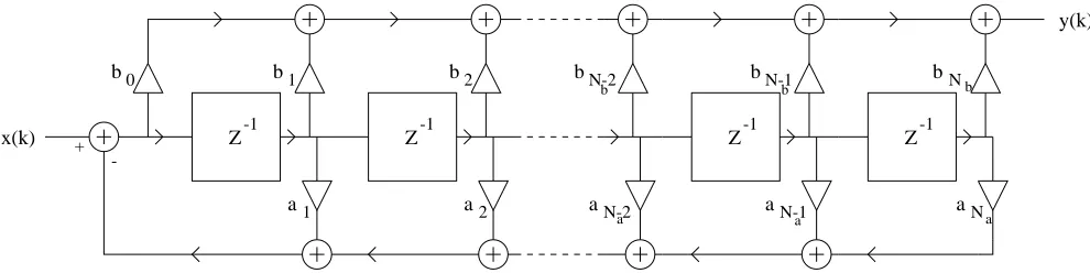
Figure 1: Structure of anNth order recursive digital filter
Use of digital filters as frequency
de-pendent boundaries in TLM
This section reviews the operation of recursive digital fil-ters and their application as frequency dependent bound-aries in TLM.
Digital filters
Digital filters are the embodiment of a set of difference equations in a sampled data system. Figure 1 shows one way of implementing a digital filter of orderN, where the orderN is the greater of the ordersNbandNa. The unit
time delay is represented by the boxes marked Z−1, the triangles labelledan orbn are coefficient multipliers, and
the circles containing a plus sign are adders (with a minus sign on an input denoting subtraction). The transfer func-tion of the filter is often described as a ratio of polynomials inZ−1. This can be used to determine the time response of the filter, by means of Z-transforms, or the frequency re-sponse of the filter by lettingZ =exp(jωTs)whereωis
the angular frequency andTsis the sampling period. For
Figure 1 the transfer function inZ−1is given in Equation 2.
H(Z) = (1)
b0+Z−1b1+· · ·Z−(Nb−1)bNb−1+Z−
Nbb
Nb 1 +Z−1a
1+· · ·Z−(Na−1)aNa−1+Z−
Naa
Na
Using the structure of Figure 1 can cause numerical prob-lems. In practice filters are often implemented as a cascade of second order sections which gives improved numerical accuracy. In order for the filter to be stable the poles of Equation 2 (zeros of the denominator) must lie inside the unit circle on the Z-plane.
Realisation of TLM boundary
The digital filter as described above has a single input and a single output. A boundary in TLM is defined by reflec-tion and transmission in two direcreflec-tions and each with two polarisations. For each boundary element, four filters must be used for transmission and four for reflection. Often the number of filters can be reduced: e.g. to model ferrite tiles [11], used as radio absorptive material against a metal
backing, only the reflection coefficients for one direction and two polarisations are required.
The Wiener-Hopf algorithm applied to
recursive design
Here the design of a least-mean-squares ‘best-fit’ filter us-ing measurement or simulation data is described. The method is based on a novel application of the Wiener-Hopf equation for signal estimators as described in [12, pp250-264]. The same method is also described by Levy [13] and used in the Matlab ‘Signal processing toolbox’ [14] rou-tines ‘invfreqz’ and ‘invfreqs’.
If we rewrite Equation 2 as:
H(Z) = B(Z)
1 +A(Z) (2)
and assume we wish to choose the coefficients ofA(Z)and
B(Z)so thatH(Z)is the best fit to the functionG(Z). The error in the fit, in the frequency domain is given by:
ǫ′(jω) =S(jω)
B(jω)
1 +A(jω)−G(jω)
(3)
whereǫ′(jω)is the error, G(jω)is the desired frequency response andH(jω)is the frequency response of the fil-ter calculated by substitutingZ = exp(jωTs)inH(Z).
S(jω)is a weighting function which can be chosen to make the problem more sensitive to errors at particular frequen-cies.
In principle the mean squared error|ǫ|2can be calculated and minimised over the desired frequency range. However
H has very non-linear dependence on the coefficients of
Aand is difficult to minimise. Widrow and Stearns [12, pp250-264] suggest an alternative formulation which over-comes this problem. If we multiply both sides of Equation 3 by(1 +A(jω))we get:
ǫ(jω) = (1 +A(jω))ǫ′(jω) (4)
= −S(jω)G(jω)−S(jω)G(jω)A(jω) + S(jω)B(jω)
If we make[ǫ]a column vector ofK samples of the error at discrete frequenciesωk, Equation 5 can be written as:
[ǫ] = [D]−[X][W] (5)
where[D]is the vector containing the product−skgk:
[D] = [−s1g1,−s2g2,· · ·,−sKgK]T (6)
[X]is the matrix combining the productsskgke−najωkTs,
na = 1, . . . Na and−ske−nbjωkTs, nb = 0, . . . Nbwhich
multiply the coefficientsanaandbnbof the filter:
[X] =
s1g1e−jω1Ts s1g1e−2jω1Ts · · · s1g1e−Najω1Ts −s1 −s1e−jω1Ts· · · −s1e−Nbjω1Ts
s2g2e−jω2Ts s2g2e−2jω2Ts · · · s2g2e−Najω2Ts −s2 −s2e−jω2Ts· · · −s2e−Nbjω2Ts
s3g3e−jω3Ts s3g3e−2jω3Ts · · · s3g3e−Najω3Ts −s3 −s3e−jω3Ts· · · −s3e−Nbjω3Ts ..
. . .. ...
sKgKe−jωKTs sKgKe−2jωKTs · · · sKgKe−NajωKTs −sK −sKe−jωKTs· · · −sKe−NbjωKTs
(7)
[W] is the vector containing the (unknown) filter coeffi-cientsanaandbnb:
[W] = [a1, a2,· · ·, aNa, b0, b1,· · ·, bNb]
T (8)
Ifℜ(x)denotes the real part ofx,[Q]T is the transpose of
[Q] and[Q]∗ is the conjugate transpose of[Q], the mean squared error is:
|ǫ|2 = 1
Kℜ {[ǫ]
∗[ǫ]}
= 1 Kℜ
[D]∗[D] + [W]T[X]∗[X][W]−
2[D][X]∗[W]}
If we let[R] =ℜ {[X]∗[X]}andP =ℜ {[X]∗[D]}then
|ǫ|2= 1
K
[D]∗[D] + [W]T[R][W]−2[P]T[W] (9)
In order to determine the minimum mean squared error we can differentiate Equation 9 with respect to the coefficient vector,[W], and equate to zero:
∂|ǫ|2
∂[W] = 1
K{2[R][W]−2[P]}= 0 (10)
This is a system of linear equations which can be solved by matrix inversion to give the filter coefficients:
[W] = [R]−1[P] (11)
Thus it is possible to design a filter to give a least-mean-squares fit to measured or computed data for a thin layer.
This technique has two potential problems:
1. The filter design is not necessarily stable.
2. The required filter order is also unknown.
The next section shows results of using the method to design filters to match reflection and transmission coeffi-cients.
Results
Perforated screen
Here the transmission coefficient of a perforated screen was simulated using a fine grid TLM model (0.1 mm) and the resulting frequency domain data used to design a transmis-sion filter for use as a boundary in a larger mesh (10 cm). A set of 50 data points were used to represent the frequency domain data (ie.K= 50). Filters of increasing order were designed and the mean squared error for a range is tabu-lated in Table 1 below. The weighting functionS= 1/|G|
was used so that the relative error tended to be the same at all frequency points. Filters of order 10 and above were unstable and therefore not used.
Poles Zeros Mean squared error Note
2 2 0.00049888
8 4 0.00024546
9 9 0.00016312
[image:5.595.196.405.42.106.2]10 10 0.00011883 Unstable
Table 1: Mean squared error for a range of ‘perforated screen’ filter designs
-60 -50 -40 -30 -20 -10 0 10
0 5e+08 1e+09 1.5e+09 2e+09 2.5e+09 3e+09
Transmission Magnitude (dB)
Frequency (Hz)
Specification Order 2,2 Order 9,9
-180 -135 -90 -45 0 45 90 135 180
0 5e+08 1e+09 1.5e+09 2e+09 2.5e+09 3e+09
Phase (deg.)
Frequency (Hz)
[image:5.595.61.285.146.309.2]Specification Order 2,2 Order 9,9
[image:5.595.320.545.151.308.2]Figure 2: Frequency response of transmission through a perforated screen (Specification) and filter designs of or-der 2 and 9.
Figure 3: Phase response of transmission through a per-forated screen (Specification) and filter designs of order 2 and 9.
Ferrite tile
The reflection coefficient of a ferrite tile was computed with TLM using a 1.05 mm grid using the technique in [1]. The Wiener-Hopf design technique was then used to compute the filter design suitable for use in a TLM model with 10 cm grid. This was also compared with the 2nd or-der approximation described in [10]. A set of 200 data points were used to represent the frequency domain data (ie. K = 200). Filters of order 3 or less produced un-satisfactory results. The first design to produce an accept-able approximation to the desired frequency response was of order 4. It was however unstable. The filter was
sta-bilised by removing the unstable pole and nearby zero, or alternatively by simply moving the unstable pole inside the unit circle such that its effect on the magnitude response was unchanged. The mean squared error for a number of designs is shown below in Table 2 below. Filters 1–3 haveS = 1/|G|however it was noticed that the zero fre-quency gain of the filter had a large error. For filters 4 and 5 the zero frequency weighting was increased by a factor of 10 which reduced the zero frequency error for a small increase in overall error (comparing filter 5 with filter 2). This demonstrated the importance of the weighting func-tion in controlling the overall error.
-15 -10 -5 -2 -10 1 2 5 10
0 5e+08 1e+09 1.5e+09 2e+09 2.5e+09 3e+09
Magnitude error (dB)
Frequency (Hz)
Order 2,2 Order 9,9
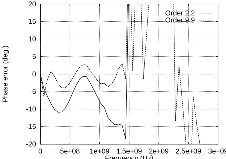
-20 -15 -10 -5 0 5 10 15 20
0 5e+08 1e+09 1.5e+09 2e+09 2.5e+09 3e+09
Phase error (deg.)
Frequency (Hz)
Order 2,2 Order 9,9
Figure 4: Magnitude error for ‘perforated screen’ filter designs of order 2 and 9.
[image:5.595.319.545.551.710.2] [image:5.595.60.288.552.713.2]No. Poles Zeros Mean squared error Note
1 4 4 0.00024291 UnstableS= 1/G
2 3 3 0.0023514 By removing pole and zero outside unit circle from 1
3 3 3 0.013959 By stabilising polynomial of 1
4 4 4 0.00030563 Unstable (changedS)
[image:6.595.93.507.42.121.2]5 3 3 0.0024013 By removing pole and zero outside unit circle from 4
Table 2: Mean squared error for a range of ‘ferrite tile’ filter designs
-40 -30 -20 -10 0 10
0 5e+08 1e+09 1.5e+09 2e+09 2.5e+09 3e+09
Reflection Magnitude (dB)
Frequency (Hz)
Specification Order 3,3 from 4,4 S=1/G Order 3,3 from 4,4 S modified 2nd order approximation
-200 -150 -100 -50 0 50 100 150 200
0 5e+08 1e+09 1.5e+09 2e+09 2.5e+09 3e+09
Reflection phase (deg.)
Frequency (Hz)
[image:6.595.319.545.172.332.2]Specification Order 3,3 from 4,4 S=1/G Order 3,3 from 4,4 S modified 2nd order approximation
[image:6.595.319.542.404.569.2]Figure 6: Frequency response of reflection from a ferrite tile absorber (Specification) and filter designs of order 2 and 3.
Figure 7: Phase response of reflection from a ferrite tile absorber (Specification) and filter designs of order 2 and 9.
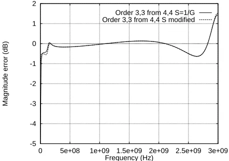
-5 -4 -3 -2 -1 0 1 2
0 5e+08 1e+09 1.5e+09 2e+09 2.5e+09 3e+09
Magnitude error (dB)
Frequency (Hz)
Order 3,3 from 4,4 S=1/G Order 3,3 from 4,4 S modified
-50 -40 -30 -20 -10 0 10 20
0 5e+08 1e+09 1.5e+09 2e+09 2.5e+09 3e+09
Phase error (deg.)
Frequency (Hz)
Order 3,3 from 4,4 S=1/G Order 3,3 from 4,4 S modified
Figure 8: Magnitude error for the ‘ferrite tile’ filter de-signs of order 3.
Figure 9: Phase error for the ‘ferrite tile’ filter designs of order 3.
Figures 6 and 7 show the frequency and phase response of the two 3rd order filters compared with the specified fre-quency response and the result of the 2nd order approxima-tion of [10]. The responses of the two 3rd order filters are almost indistinguishable at this resolution. It can be seen that the Wiener-Hopf design is slightly more accurate than the 2nd order approximation at higher frequencies. How-ever phase information is required for the Wiener-Hopf de-sign which must be measured or determined by simulation
whilst the 2nd order approximation can be computed from the magnitude of the tile’s reflection coefficient only. Fig-ures 8 and 9 show the error in the magnitude and phase response of the 3rd-order filters as a function of frequency.
Conclusions
[image:6.595.60.289.409.570.2]com-puted frequency response (phase and magnitude). However the order of the filter must be determined experimentally and sometimes manual interaction is required to stabilise the filter.
The algorithm will find application in the modelling of thin lossy layers, such as composite materials, where the transmission and reflection coefficients can be measured or computed in the frequency domain.
The filter based boundary conditions have been installed in the ”Hawk” TLM package at York and demonstrated for ferrite tiles [11, 10] and thin conducting layers [6] us-ing analytical formulations approximatus-ing the frequency response of reflection and transmission. The new technique described here allows boundaries to be formulated for lay-ers using measured or computed data where a sutiable ana-lytical formulation is not available.
Acknowledgments
The authors would like to thank British Aerospace, Lucas Varity, EPSRC, D.G. Teer Coatings who have supported this work.
References
[1] J.F. Dawson. Improved magnetic loss for TLM. Elec-tronics Letters, 29(5):467–468, 1993.
[2] A. Mallik and C. P. Loller. The modelling of EM leakage into advanced composite enclosures using the TLM technique. International Journal of Numerical Modelling, Electronic Networks, Devices and Fields, 2(4):241–248, 1989.
[3] D.P. Johns, J. Wlodarczyk, and A. Mallik. New TLM models for thin structures. In IEE Proc. Interna-tional Conference on Computation in Electromagnet-ics, pages 335–338, 1991.
[4] V. Trenkic, A. P. Duffy, T. M. Benson, and C. Christopoulos. Numerical simulation of penetra-tion and coupling using the TLM method. In EMC’94 Roma, pages 321–326, 13–16 September 1994.
[5] Ch. Fuchs and A. J. Schwab. Efficient computation of 3D shielding enclosures in time domain with TLM. In COST 243 Workshop, Numerical Methods and their Applications, Hamburg, June 1995.
[6] J. A. Cole, J. F. Dawson, and S. J. Porter. Efficient modelling of thin conducting sheets within the TLM method. In IEE 3rd Int. Conference on Computation in Electromagnetics, Bath, 10–12 April 1996.
[7] K.S. Kunz, D.J. Steich, and R.J. Luebbers. Low fre-quency shielding effects of a conducting shell with an aperture: Response of an internal wire. IEEE Trans-actions on Antennas and Propagation, pages 370– 373, 1992.
[8] L.-K. Wu and L.-T. Han. Implementation and applica-tion of resistive sheet boundary condiapplica-tion in the finite-difference time-domain method. IEEE Transactions on Antennas and Propagation, pages 628–632, 1992.
[9] J.G. Maloney and G.S. Smith. A comparison of meth-ods for modelling electrically thin dielectric and con-ducting sheets in the finite-difference time-domain (FDTD) method. IEEE Transactions on Antennas and Propagation, pages 690–694, 1993.
[10] J.F. Dawson, J. Ahmadi, and A. C. Marvin. Mod-elling the damping of screened room resonances by ferrite tiles using frequency dependent boundaries in TLM. In IEE 2nd Int. Conf. on Computation in Elec-tromagnetics, pages 271–274, 1994.
[11] J.F. Dawson. Representing ferrite absorbing tiles as frequency dependent boundaries in TLM. Electronics Letters, 29(9):791–792, 1993.
[12] B Widrow and S. D. Stearns. Adaptive signal process-ing. Prentice-Hall, 1985. ISBN 0-13-004029-01.
[13] E. C. Levy. Complex curve fitting. IRE Trans. on Automatic Control, AC-4:37–44, 1959.
[14] T. P. Krauss, L. Shure, and J. N. Little. Signal pro-cessing toolbox for use with Matlab. The Mathworks Inc., 1994.