Numerical solutions for unsteady gravity-driven flows in collapsible tubes: evolution and roll-wave instability of a steady state

This is a repository copy of

Numerical solutions for unsteady gravity-driven flows in

collapsible tubes: evolution and roll-wave instability of a steady state

.

White Rose Research Online URL for this paper:

http://eprints.whiterose.ac.uk/1237/

Article:

Brook, B.S., Falle, S.A.E.G. and Pedley, T.J. (1999) Numerical solutions for unsteady

gravity-driven flows in collapsible tubes: evolution and roll-wave instability of a steady

state. Journal of Fluid Mechanics, 396. pp. 223-256. ISSN 0022-1120

[email protected] https://eprints.whiterose.ac.uk/

Reuse

Unless indicated otherwise, fulltext items are protected by copyright with all rights reserved. The copyright exception in section 29 of the Copyright, Designs and Patents Act 1988 allows the making of a single copy solely for the purpose of non-commercial research or private study within the limits of fair dealing. The publisher or other rights-holder may allow further reproduction and re-use of this version - refer to the White Rose Research Online record for this item. Where records identify the publisher as the copyright holder, users can verify any specific terms of use on the publisher’s website.

Takedown

If you consider content in White Rose Research Online to be in breach of UK law, please notify us by

c

1999 Cambridge University Press

Numerical solutions for unsteady gravity-driven

flows in collapsible tubes: evolution and

roll-wave instability of a steady state

By B. S. B R O O K1, S. A. E. G. F A L L E2

A N D T. J. P E D L E Y3

1_{Department of Medical Physics and Clinical Engineering, University of Sheffield,} Royal Hallamshire Hospital, Sheffield, S10 2JF, UK

2_{Department of Applied Mathematical Studies, University of Leeds, Leeds, LS2 9JT, UK} 3_{Department of Applied Mathematics and Theoretical Physics, University of Cambridge,}

Silver Street, Cambridge CB3 9EW, UK

(Received 29 September 1998 and in revised form 15 May 1999)

Unsteady flow in collapsible tubes has been widely studied for a number of different physiological applications; the principal motivation for the work of this paper is the study of blood flow in the jugular vein of an upright, long-necked subject (a giraffe). The one-dimensional equations governing gravity- or pressure-driven flow in collapsible tubes have been solved in the past using finite-difference (MacCormack) methods. Such schemes, however, produce numerical artifacts near discontinuities such as elastic jumps. This paper describes a numerical scheme developed to solve the one-dimensional equations using a more accurate upwind finite volume (Godunov) scheme that has been used successfully in gas dynamics and shallow water wave problems. The adapatation of the Godunov method to the present application is non-trivial due to the highly nonlinear nature of the pressure–area relation for collapsible tubes.

The code is tested by comparing both unsteady and converged solutions with analytical solutions where available. Further tests include comparison with solutions obtained from MacCormack methods which illustrate the accuracy of the present method.

Finally the possibility of roll waves occurring in collapsible tubes is also considered, both as a test case for the scheme and as an interesting phenomenon in its own right, arising out of the similarity of the collapsible tube equations to those governing shallow water flow.

1. Introduction

inference that the flow resistance of the jugular vein is high and therefore that the vein is highly collapsed in upright posture. Given a constant right atrial pressure, we have predicted that, for steady flow, an unusual flow limitation can occur (Pedley, Brook & Seymour 1996). For a jugular vein with uniform elastic and geometric properties, the steady solution that most closely matches intravascular pressure measurements is one in which the flow is supercritical at the exit from the skull (i.e. the fluid velocity exceeds the speed of propagation of small-amplitude pressure waves). The constant right atrial pressure at the downstream end, however, forces the flow to be subcritical there. The only way in which flow can be decelerated from supercritical to subcritical velocities is via an elastic jump. If the flow rate exceeds a certain maximum, even the existence of an elastic jump does not allow the downstream boundary condition to be satisfied and therefore steady flow cannot exist. We wish to discover what happens in that case and, in particular, whether steady flow limitation emerges as a stable final state from different initial conditions. Of further interest is the nature of the flow in the jugular vein during time-dependent manoeuvres such as raising the head quickly after the giraffe has put its head down to drink. A large volume of blood is sequestered in the (distended) veins in the neck while the head is down and on raising the head this large volume of blood would be accelerated back to the heart. Does some kind of flow limitation come into action in this case?

In order to answer such questions a stable, accurate numerical method is needed to solve the equations governing one-dimensional unsteady flow in a collapsible tube. The numerical code is developed and tested in this paper; detailed application to the giraffe jugular vein will be made in a separate paper. In some of the most recent stud-ies (Kimmel, Kamm & Shapiro 1988; Elad & Kamm 1989; Eladet al. 1991; Kamm & Dai, personal communication), the time-dependent equations have been integrated numerically using a finite-difference method (MacCormack’s scheme). However, the governing equations form a system of nonlinear hyperbolic partial differential equa-tions. Typically in such systems discontinuous solutions develop and propagate even if the initial data are smooth. The MacCormack method uses both downwind and up-wind differencing and therefore produces oscillations near discontinuities, which can be removed only by adding a large amount of artificial dissipation (Roe 1986), which could suppress physical oscillations as well as numerical ones. The wavy structures are evident in the numerical simulations by Elad et al. (1991) as shown in figure 6 below (where artificial dissipation has not been added). We have chosen instead to use an upwind shock-capturing scheme of the type first proposed by Godunov (1959). Such methods require a solution to a Riemann problem with discontinuous initial data and an exact solution to this is non-trivial. The second-order Godunov scheme described by Falle (1991) works well for this system and has the further advantage that it is possible to impose the correct boundary conditions at the ends of the tube.

Hydraulic jump

Subcritical

Supercritical

Channel bed

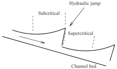
Figure 1.Schematic illustration of roll waves down an inclined open channel.

the velocity of the fluid is everywhere less than the roll wave speed. Using the shallow water wave equations augmented by the Chezy drag (modelling the flow resistance), Dressler (1949) showed that, when the steady uniform flow down an inclined channel was unstable, periodic solutions could be constructed that resembled roll waves, with a smooth transition from sub- to supercritical flow followed by a hydraulic jump allowing transition back to subcritical flow (see figure 1). Needham & Merkin (1984) modified the equations governing shallow water flow by including a viscous dissipative term and showed that continuous roll-wave solutions could be obtained from these modified equations. Cowley (1981) demonstrated the existence of roll-wave solutions to the collapsible-tube equations, and constructed an actual solution for a particular form of the tube law and (turbulent) resistance function R. The shape of the constructed waves was generally similar to those produced by Dressler for roll waves in channels. The code we have developed enables us to decide whether roll waves can arise spontaneously out of perturbations to an unstable steady flow. The question is relevant because the anaylsis carried out by Cowley assumes a quasi-steady roll-wave solution, and the analysis of the time-dependent nonlinear equations was not considered. The code solves the nonlinear equations and thus can be used to investigate the evolution of the quasi-steady flow.

2. Governing equations

Conservation of mass for an incompressible fluid requires that

∂A ∂t +

∂uA

∂x = 0 (2.1)

where A=A(x, t) is the cross-sectional area of the tube, u=u(x, t) is the velocity of the fluid, averaged across the cross-section, and x is measured along the tube in the direction of the flow.

Conservation of momentum gives

∂u ∂t +u

∂u ∂x+

1

ρ ∂P ∂x +

1

ρR(A, u)uA−g= 0, (2.2)

the resistance term linearly (i.e. neglecting convective inertia or turbulence) as

R = 8πµA 1/2

o

A5/2 , (2.3)

whereµis the viscosity of blood andAo is the undistorted cross-sectional area of the tube, which can be a function of x. If the tube remained circular as it collapsed the resistance term would be simply the Poiseuille formula R = 8πµ/A2_{. However, the} cross-section of a collapsible tube typically takes on an elliptical shape and finally a dumbbell shape. Equation (2.3) is an approximation to the formula for an elliptical cross-section; the important property of the chosen function is that the resistance increases more rapidly as the area decreases than it would in a circular tube.

Finally, the pressure in the collapsible tube is related to the area via a simple tube law. Experiment and theory have shown that the pressure–area relations of uniform elastic tubes of a variety of sizes and wall thicknesses, but made of the same material, can be roughly described by the following equation:

P₋Pe=KpF(A/Ao), (2.4)

where P is the internal pressure, Pe is the external pressure, and Kp is the bending stiffness of the tube (Shapiro 1977). The functionF in (2.4) is called the tube law. For a thin wall made from a homogeneous linearly elastic material Kp is given by

Kp =

E

12(1₋σ2₎1/2

h r

3

, (2.5)

where E and σare the Young’s modulus and Poisson’s ratio of the material and h/r

is the wall thickness to radius ratio when the tube is circular and not distended. We take the functionF(A/Ao) to have the form

F(α) =α10₋α−3/2, whereα=A/Ao, (2.6) which is a continuous function combining great stiffness for α > 1 with a known similarity solution as α_→0 (cf. Elad, Kamm & Shapiro 1987). In practice, properties such as the undistorted area, wall stiffness, and external pressure may all vary with distance down the vein. In order to model this variation, we shall allow Ao, Kp, and

Pe to be functions of longitudinal distancex.

The equations (2.1) and (2.2) with (2.3) and (2.4) form a system of nonlinear hyper-bolic partial differential equations. Typically in such systems discontinuous solutions develop and propagate. For simple cases it is possible to obtain analytical solutions using the method of characteristics. In this case however the high nonlinearity of the tube law (2.6) and the variation in Ao, Kp, and Pe down the vein rule out analytical solutions.

3. Numerical scheme

3.1. Derivation of equations in conservative form

Equations (2.1) and (2.2) are two nonlinear conservation laws for the quantitiesαand

Uα. Numerical schemes for such systems should be conservative so that the correct jump conditions are automatically satisfied at shocks (i.e. elastic jumps). It should also be upwind biased if the scheme is to have the same boundary conditions as the original equations. For instance, if the downstream boundary condition is such that the pressure at the outlet is to remain fixed, then the nature of the characteristics and the direction in which information is propagated is important. Using an upwind scheme enables us to retain the direction of information propagation in implementing the boundary conditions. Equations (2.1) and (2.2) are therefore rewritten in the following conservative form:

∂V

∂τ + ∂F

∂ξ +S = 0, (3.1)

where V _{is a solution vector,}F _{is a vector of fluxes,} S _{represents the source terms,} and τ, ξ represent time and space variables. Equation (2.1) is already in this form, and the momentum equation (2.2) can be rewritten as follows (see Elad et al. 1991):

∂ ∂t(uA) +

∂ ∂x

A

u2+P −Pe

ρ

− K_ρp

Z

FdA

+A

ρ

dPe dx +

1

ρ

Z

FdAdKp

dx −gA+

1

ρA

2_{R(A)u= 0. (3.2)}

We define the following non-dimensional variables, in addition toα=A/Ao:

ξ=x/L, τ=cot/L, C=c/co, U =u/co, R˜(α) =R(A)/R(Ao), (3.3) where Ao is the undistorted area, L is the length of the vein, co is a characteristic wave speed given by c2

o = Kp/ρ and the non-dimensional viscous resistance works out as ˜R(α) = α−5/2_{. These variables are valid only for a uniform tube because, in} the case of non-uniform tubes, Ao andKp will vary with longitudinal distance. Using these non-dimensional variables we can now combine (2.1) and (3.2) into the form (3.1) where, for a uniform tube,

V ₌ α Uα , (3.4) F ₌ Uα αU2_{+αF(α)−Γ}

, (3.5)

whereΓ =R

F(α) dα, and

S ₌  

0

−_ρcαL2

o

(ρg₋RUαR˜ ocoAo) 

. (3.6)

HereRo is the resistance at the uncollapsed area, i.e.R(Ao).

For a non-uniform tube, the forms of the vectors have to be modified to

F ₌  

UαAo

αAoU2+

KpAo

ρc2

o

(αF(α)₋Γ) 

, (3.8)

and

S ₌  

0

Ao

ρc2

o

αdPe

dξ +Γ

dKp dξ

− αA_ρco2L

o

(ρg₋RUαR˜ ocoAo) 

. (3.9)

3.2. Scheme construction

To construct a scheme for equations (3.1), the computational domain is divided into equal cells with mesh spacing ∆ξ. That part of the tube for which ξj−1 6ξ 6 ξj is then the jth cell and

∆ξ=ξj−ξj−1. (3.10)

Thejth cell also has interfaces atj₋1₂ andj+1

2 so thatξj−1= (j− 1

2)∆ξ. Integrating equations (3.1) over the jth cell thus gives

(ξj−ξj−1) d dτVj+

1

∆ξFj+1/2−Fj−1/2=Sj, (3.11)

where the flux vectorF_{j−1/2, for example, is the flux at the interface between cellj−1} and cellj.

V_{j =} 1 ∆ξ

Z ξj

ξj−1

V_{dξ (3.12)}

is the mean value ofV _{in thejth cell and}

S_{j =} 1 ∆ξ

Z ξj

ξj−1

S_{dξ (3.13)}

is the mean value of the source term in the jth cell. Equations (3.11) are exact and express conservation of the quantities in V_{. A conservative scheme can now be} constructed by choosing suitable approximations to the flux and source terms and integrating over a time step to get

V_jk+1−V_{jk+ (}F_j+k/2+1/2−F_j−k/2+1/2)∆τ

∆ξ = ∆τSjk+1/2, (3.14)

where the solution at time step k in cell j is denoted by V_jk, F_{j+k/2+1/2 and} S_jk+1/2 are the mean values ofF_{j+1/2 and} S_{j over the time step and}

∆τ=τk+1−τk. (3.15)

3.3. Discretization and solution procedure

The second-order Godunov scheme is an explicit second-order finite-volume scheme (Harten, Lax & Vanleer 1983; Roe 1986). It is designed to capture elastic jumps, and is upwind biased. The following are the main steps in the procedure:

(a) The Eulerian grid is divided intoN equal-length space cells (along theξ-axis), and T time cells, where T is a variable and is determined by convergence criteria.

First the solution at time k+1

2 is calculated, using a first-order step, via

V_jk+1/2=V_jk− ∆τ

2∆ξ(Fj+k/2+1/2−Fj−k/2+1/2) +

∆τ

2 Sjk. (3.16) The fluxes are determined by ignoring the source terms and solving a Riemann problem locally at the boundaries of the cells. A Riemann problem for a hyperbolic system such as (3.1) with no source terms (i.e. S _{= 0) is defined to be an initial value} problem with discontinuous initial data of the form

V_{(0) =} (

V_{l = const to the left of the interface}

V_{r= const to the right of the interface.} (3.17) The Riemann problem is essentially the same as the shock-tube problem of gas dynamics and the dam-break problem of shallow water waves in open channels. Any initial discontinuity in flow variables across an interface that separates two uniform states breaks up into left and right moving waves (with respect to the fluid). Each wave can be either a shock or a rarefaction. Thus in the scheme above we require the solution V∗₍V_l,V_{r), i.e. the state of the flow variables at the interface at some} time after the breakup of the initial discontinuity. The Riemann solver should thus calculate the position and type of the left and right waves that result from the breakup and the state at the interface, which remains constant after the initial breakup. (See figure 2). So if the solution to the Riemann problem is V∗₍V_l,V_{r) then the fluxes are} calculated viaF ₌F₍V∗_{). This is done at all cell interfaces so that in general}

F_{j−k/2+1/2 =}F₍V∗₍V_j−1k,V_{jk)). (3.18)} The Riemann problem solution procedure used here is described in greater detail in the Appendix.

(c) Second-order step – The second-order step is now constructed using the solution at half-time, V_{jk+1/2. We construct a gradient}G_{jk+1/2 in each cell which is given by}

G_{jk+1/2= Av} V_jk+1/2−V_j−1k+1/2,V_j+1k+1/2−V_jk+1/2

, (3.19)

where Av(a, b) is an averaging function.

It would be desirable to have a scheme that is second-order accurate everywhere as would be the case if a straight average is used in (3.19). However, Godunov’s theorem says that such a scheme would generate oscillations in places where the second derivative becomes large (e.g. elastic jumps). Thus an averaging function is chosen such that the average gradient is biased towards the smaller of the two values in such places, giving only first-order accuracy locally. We set the averaging function to be

Av(a, b) = a

2_b+b2_a

a2_+b2 for ab >0 Av(a, b) = 0 forab <0.

    

(3.20)

The gradients are now used to set up a Riemann problem for the second-order step so that

V_{l =}V_jk+1/2+ 1

2Gjk+1/2, Vr=Vj+1k+1/2− 1

2Gj+1k+1/2. (3.21) Thus the second-order flux is given by

These fluxes are now used to update the solution over the whole time step, so that

V_{jk+1 =}V_jk− ∆τ

∆ξ(Fj+k/2+1/2−Fj−k/2+1/2) + ∆τSjk+1/2. (3.23)

(d) The second-order source terms are obtained from the solution at half-time, V_jk+1/2.

(e) The stability condition (which is calculated at the beginning of each time step) is

∆τ6 ∆ξ maxjn|λjn|

, n= 1,2, (3.24)

whereλj1=uj−cj andλj2 =uj+cj.

4. Test cases

As with any numerical scheme, for there to be confidence in physical interpretations based on the numerical results, a number of tests need to be carried out to show that the solutions obtained using the code are in good agreement with exact known solutions. The exact solutions in most cases are calculated analytically. However, the nature of the tube law for the collapsible tube equations means that analytical solutions are not possible. Thus, we use a variety of different test examples.

First, we adapt the code to solve the shallow water version of the problem and then compare the results with analytical solutions, which in this case are possible. We then pick an artificial, highly nonlinear tube law. It is artificial in that it does not correspond to any biological or physical material but it still permits an analytical solution. In both cases we solve the one-dimensional dam-break (or shock-tube) problem in which initially two stationary bodies of fluid at different depths are separated by a barrier (Whitham 1974). The barrier is removed (or the dam breaks) instantaneously and the subsequent fluid flow is calculated. This is of course a Riemann problem which is solved at every interface in the Godunov scheme. Finally in this section, we also compare results obtained using the Godunov scheme for collapsible tubes and those obtained using the MacCormack schemes; in particular, we examine calculations from the numerical studies of Eladet al. (1991).

A more direct means of comparison is one in which we compare the converged solutions obtained using the Godunov scheme, as described here, with the steady solutions found as described by Pedley et al.(1996). Clearly, this is sufficient as far as the converged solution goes, but it is necessary to carry out the tests described above to ensure that the intermediate unsteady results are reliable as well.

4.1. Analytical and numerical solutions for the shallow water equations

The equations governing one-dimensional unsteady flow in open channels are exactly analogous to the collapsible tube equations and are usually written as follows:

∂h ∂t +

∂

∂x(hu) = 0, (4.1)

and

∂u ∂t +g

∂h ∂x+u

∂u

∂x = 0, (4.2)

the distance along the channel. The momentum equation (4.2) is the same as the collapsible tube equation (2.2) if we take P as the hydrostatic pressure P =ρghand zero viscous resistance. The corresponding ‘tube law’ for the shallow water equations is given by

F(h) =h. (4.3)

Analytical solution to the one-dimensional dam-break problem

This is a standard problem, the solution to which is described fully by Whitham (1974). Here we state the problem and simply quote the solutions. Equations (4.1) and (4.2) can be written as

∂P

∂t +A ∂P

∂x = 0, (4.4)

where

P ₌

h u

, (4.5)

and

A=

u h g u

. (4.6)

Ahas eigenvaluesλ1,2=u±cwherec=√gh,with the corresponding left eigenvectors

l_{1,2 =}

±p

g/h

1

, (4.7)

so that

l_i·

∂P

∂t +λi ∂P

∂x

= 0. (4.8)

The Riemann invariants are given by

R±=u±2c, (4.9)

and are constant along the characteristic curves defined by dx/dt=u_±c.

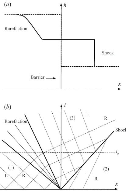
Consider now the initial state in which fluid of different depths is separated by a barrier. We calculate the fluid flow after the barrier is removed. Suppose the water to the left of the barrier has depthh1 and that to the right has depth h2, whereh1> h2. On removal of the barrier, a shock will propagate to the right and a rarefaction to the left as shown in figure 2(a). The corresponding x, t diagram showing the characteristics is as depicted in figure 2(b). The undisturbed fluid upstream of the rarefaction is labelled region (1), the undisturbed fluid downstream of the shock is labelled region (2), and the disturbed fluid in between the rarefaction and shock is labelled region (3).

In the region x <0, t <0, the fluid is at rest and c is a constant,c1 =√gh1. The water depths h1 and h2 are known and u1 = u2 = 0. The wave speed in the fan is given by

cr = 13(2c1−x/t) (4.10)

and the fluid speed in the fan is therefore

Rarefaction

Barrier

Shock

(a) h

x

Rarefaction (3)

Shock

(b) t

x

L R

(2)

L R

(1)

R

t_e

Figure 2.(a) A schematic of the pressure (or water height) profile for the shock-tube (or dam-break) problem in which the initial left and right states for the gas pressure (or water depth) are shown by the dashed line. If the initial velocity on both sides of the barrier is 0, then we would expect a shock to propagate to the right and a rarefaction to the left. The possible solution at a later time

te is indicated by the solid line. (b) The correspondingx, tdiagram. L and R indicate the left and right characteristics respectively.

The shape of the free surface in the fan is then found from (4.10) so that

hr = 1 9g(2

p

gh1−x/t)2. (4.12)

The water depth, h3, in the disturbed region is given by the solution to 8h2h3(h1+h3−2

p

h1h3) = (h2−h3)2(h2+h3). (4.13) The fluid speed in the disturbed region is then determined via

u3 = 2c1−2c3 = 2√g(ph1−

p

h3), (4.14)

and the shock speed is given by

u2s = 12g

h3

h2

(h2+h3). (4.15)

(b)

x

0.2 0.4 0.6 0.8 1.0

0 0.2 0.4 0.6 0.8 1.0

F

roude number

,

S

=

u

/

c

(a)

10 20 30 40

Depth of w

ater abo

v

e channel

bed

, (

h

)

0

Nonlinear Linear Analytical

x

0.2 0.4 0.6 0.8 1.0

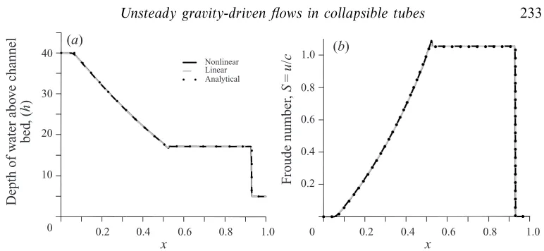
Figure 3.Solutions to the dam-break problem atte= 0.0: (a) the shape of the free surface and (b) the Froude number (fluid velocity/wave speed) versus distance. The different line types are for the three different methods of solution as indicated in the text.

the values of h3 and u3. Obviously the position of the rarefaction and shock will depend on the time tand so, for comparison with the numerical results, we calculate the analytical solution at a particular time te and stop the numerical computation at this time as well. When appropriate non-dimensionalization is used (as in (3.3) with

c2

0 =gh0) equation (4.13) is unchanged, the g drop out of (4.12) and (4.15), and we also have

u2₃ = 1 2h2h3

(h2−h3)2(h2+h3). (4.16)

We use the initial condition as shown in figure 2(b) to solve the dam-break problem numerically so that in the analytical solution we will only need to use the following data: h1 = 40.0, h2 = 5.0, u1=u2 = 0.

The numerical procedure is exactly as described in the Appendix except of course the flux vectors, ‘tube law’ and wave-speed expressions are different. We use both a linear Riemann solver and a nonlinear Riemann solver to show that in the shallow water case a linear solver is sufficient for good agreement with the exact solution. The linear solver is basically as described in the Appendix except that the first guess denoted p∗

0 is taken to be the resolved state. Thus no iterations are carried out to get p∗ _{closer to the exact solution. The mesh size ∆ξ = 0.001 and a time step} ∆τ= (0.8∆ξ)/(max_|λi|) were used for the solutions shown.

As shown in figures 3(a) and 3(b), the agreement is very good between the solutions calculated using both the linear and nonlinear Riemann solver and those calculated analytically. A coarser mesh (∆ξ = 0.01) gives very similar results except that the shock is not resolved as accurately as in the cases shown. The overshoot in figure 3(b) is a non-physical artefact that diminishes with a finer mesh size (∆ξ= 1/1500). This is consistent with the fact that truncation errors reduce with decreasing mesh size.

4.2. Solutions for a nonlinear artificial tube law

We now turn to an artificial tube law that is highly nonlinear but analytically tractable, i.e.

(a)

Distance along vein, ξ 1.2

0 0.2 0.4 0.6 0.8 1.0

Speed inde x, S = u / c Nonlinear Analytical 1.3 1.4 1.5 1.6

Cross-sectional area of the v

ein,

α

(b)

Distance along vein, ξ 0.02

0 0.2 0.4 0.6 0.8 1.0

0.04 0.06 0.08 0.10 0.12

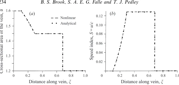
Figure 4.Solutions to the shock-tube problem at τe = 0.012: (a) the cross-sectional area of the tube, and (b) the speed index (fluid velocity/wave speed), against distance along the vein using the two different methods of solution as indicated in the text.

The non-dimensional wave speed is therefore

c(α) =√10α5. (4.18)

Following the same arguments as in_§4.1, we obtain the following non-dimenionalized analytical solutions to the shock-tube problem. The cross-sectional area of the tube

α3 in region (3) is determined from the equation

11α2α3(α51−α53)2−25(α112 −α113 )(α2−α3) = 0. (4.19) The fluid velocity in region (3) is given by

u3 =

√ 10 5 (α

5 1−α

5

3), (4.20)

and the shock speed is obtained via

us= ₁₀

11

α3

α2

α11 2 −α113

α2−α3

1/2

. (4.21)

Solutions within the rarefaction fan are then

αr= ₁

6√10

c1−5

ξ τ

1/5

, (4.22)

ur= 1 6

√ 10α51+

ξ τ

. (4.23)

The code is again adapted to take into account the different tube-law and wave-speed expressions; a nonlinear Riemann solver was used. Figures 4(a) and 4(b) show typical solutions to the shock-tube problem for the initial data, α1 = 1.6, α2= 1.2,

u1 =u2= 0.

step, because the approximate solutions p∗

0 are too far from the exact answer p∗. This indicates that the investigation into the jugular vein problems will require the nonlinear Riemann solver.

4.3. Comparison with MacCormack schemes

The MacCormack scheme has been used for solving one-dimensional flow problems in collapsible tubes with application to expiration (Kimmel et al. 1988; Elad & Kamm 1989) and more recently to external vein compression (R. D. Kamm & G. Dai, personal communication). The advantages of the Godunov scheme over the MacCormack scheme have been discussed. It now remains to show how the results from the code we have developed compare with those obtained using the MacCormack scheme.

A problem that has been investigated using collapsible tube models is that of flow limitation in the airways during forced expiration. First we consider the results presented by Eladet al.(1991). The governing equations are cast into the conservative form (3.1) for which the solution vectors, flux vectors and source terms are given by (3.4),

F ₌  

Uα

αU2₊ Kp

ρc2

o

(αF(α)₋Γ) 

, (4.24)

and

S ₌  

0 1

ρc2

o

αdPe

dξ +Γ

dKp dξ

+fU2



. (4.25)

Note that Kp here may be a function of ξ and therefore not equal to ρc2o. In this formulation there are no gravity terms and viscous resistance is introduced via a wall shear stress, which gives rise to the friction parameter f= 2fTL/D0 where fT is the skin friction coefficient and D0 is the unstressed diameter. The boundary conditions used by Eladet al. are very different to those in the examples shown above. Initially there is no flow through the tube, and then the downstream cross-sectional area, and hence the pressure, are perturbed from an initially undistorted area and pressure for a short time T0. A pressure gradient is thus created which drives flow through the tube.

For this example, the tube was assumed to be uniform so that A0 = 4 cm2. The external pressure was taken to be zero and the stiffness was taken to vary longitudinally so that

Kp(ξ) =Kp0exp (Ckξ) (4.26) where the values Kp0= 50 Pa andCk= 1.8 were used. The form of stiffness variation in (4.26) allows a smooth sub- to supercritical transition. The code is adapted to solve the equations with the relevant changes and the results are shown in figures 5(a) and 5(b). These should be compared with those obtained via the MacCormack method shown in figure 6 from Eladet al. (1991).

The differences between the results for the MacCormack schemes and Godunov scheme are as follows:

(i) There are no non-physical oscillations downstream of the elastic jump, but such oscillations are clearly evident in the solutions obtained via the MacCormack scheme (figure 6a).

(a)

Distance down the airway, ξ 0.2

0 0.2 0.4 0.6 0.8 1.0

Speed inde

x,

S

(

u

/

c

)

Converged steady solution 0.4

0.6 0.8 1.0

Cross-sectional area,

α

(b)

Distance along vein, ξ 0.2

0 0.2 0.4 0.6 0.8 1.0

0.4 0.6 0.8 1.0 1.2

Converged steady solution

Figure 5.(a) Cross-sectional area and (b) speed index, versus distance down the airway. The dashed line indicates the initial condition while the solid lines indicates the solution at subsequent time steps. Note the smooth transition throughS= 1 in (b).

(a)

ξ 0.1

0 0.5 1.0

0.5 1.0

α

(b)

ξ

0 0.5 1.0

0.5 1.4

S

1.0

3000

500

400

300

200 100

Figure 6.Results of the numerical solution of a supercritical flow through a uniform tube. Evolution in time is indicated by the number of iterations and computation was carried out until steady state was reached. Solutions were obtained via the MacCormack scheme using equations (3.4), (4.24) and (4.25). All solutions in this figure are taken from Eladet al.(1991).

between the wave speed as determined via the MacCormack scheme and that calcu-lated by the Godunov scheme (figure 5) in that the waves in figure 6 have already propagated upstream within the time T0 thus affecting the nature of the transient solutions.

5. Linearized theory and roll-wave instability

and resistive forces balance and the flow is necessarily supercritical in this case; steady subcritical flows are not uniform (see Pedley et al.1996).

The equations governing one-dimensional flow down a collapsible tube are as described above and in non-dimensional form are

∂α ∂τ +

∂

∂ξUα= 0, (5.1)

∂U ∂τ +U

∂U ∂ξ +C

2∂α

∂ξ +Rw(α, U)− ρgL

c2

o

= 0, (5.2)

whereRw(α, U) is the non-dimensional resistance term,

Rw(α, U) = 8πµL

ρcoAo

Uα−3/2. (5.3)

The resistance term satisfies the following conditions as specified by Cowley (1982):

Rw(α,0) = 0, (5.4)

and

∂Rw

∂α <0, ∂Rw

∂U >0 for U>0, (5.5)

and is analogous to the Chezy drag in the shallow water equations. Three relevant local wave speeds can be identified from these equations. Two of these are the wave speeds of small-amplitude dynamic pressure waves, calculated on the assumption that gravity and friction can be neglected:

C±=U±C (5.6)

where

C2=α∂F(α)

∂α . (5.7)

Kinematic waves which occur when there is an approximate balance between gravity and friction give rise to the third wave speed of very long-wavelength kinematic waves. This is given by

C1=U

1₋ α ∂Rw/∂α

U∂Rw/∂U

. (5.8)

For the resistance given by (5.3), (5.8) reduces to

C1= 5₂U. (5.9)

In our case the steady supercritical uniform solution is given by the balance between the gravitational and viscous forces. The area at which this occurs is αlim, such that

αlim=α∗ = ₈

πµQ gA2

o 2/5

(5.10)

and

U∗ = Q

Aocoα∗

. (5.11)

(1974) imposed a small pertubation to the steady solutions so that

α=α∗+a′(ξ, τ) (5.12)

(where the starred quantity represents the steady solution and the primed quantity the perturbation), linearised the equations, and deduced that the disturbance grows unless

U∗₋C∗< C1∗< U∗+C∗, (5.13) which for the specific resistance term (5.3) reduces to

−2 3 < S

∗_< 2

3. (5.14)

It seems surprising that instabilities would appear in subcritical flow (2₃ < S∗ < 1), but it should be remembered that the form of resistance we have chosen to use may not be physically accurate and this critical value for S∗ depends crucially on the resistance law. We would however expect instability to occur in supercritical flow; this is certainly the case for flows down open inclined channels where the critical Froude number for instability is F = 2. In any case, when the inclined collapsible tube is collapsed, flow velocities are highly supercritical and thus for the present investigation it suffices to consider only the flow regime in whichS∗_>1.

Quantitative comparisons can be made between the growth rate obtained from the linearized theory and results for growth rate that can be obtained via the numerical code. In order to do this we require a general wavenumber-dependent expression for the growth rate of small perturbations. We assume a solution of the form

a′=Aei(kξ−ωτ)_{, (5.15)}

where k is the wavenumber andω=ωR+ iωI. Substituting fora′ into the linearized equations gives the following dispersion relation:

ω2+βω+γ= 0 (5.16)

where

β=₋2U∗k+ ˜qα∗−3/2i, (5.17)

γ= (U∗2_−C∗2_)k2₋ 5 2˜qU∗α∗−

3/2_{ki, (5.18)}

and

˜

q= 8πµL

ρcoAo

. (5.19)

From equation (5.15), we see that a plot of the natural logarithm of the amplitude of a disturbance of wavenumber k, versus time, should yield a straight line graph with gradient ωI. We therefore require an expression for ωI from the above theory. Writing

β2₋4γ= ˜reiθ_{, (5.20)}

we obtain

ωI =−1₂q˜+ ₂1˜r1/2sin1₂θ. (5.21)

We may note that the above linear theory can be extended to a weakly nonlinear theory, using multiple scales (Dodd et al. 1982), which shows as expected that the front of the growing wave steepens as it propagates. For the corresponding water-wave problem, Yu & Kevorkian (1992) showed that, if the Froude number U∗_/C∗ _{is only} slightly above its critical value of 2, a weakly nonlinear solution can be found which remains uniformly valid at large times and tends to the Dressler (1949) discontinuous solution. They also showed that the wavelength of the roll waves is the same as that of the initial disturbance, so their theory did not shed any light on how the roll-wave wavelength is selected in practice.

6. Numerical investigation of instability

We now impose a small perturbation on a steady uniform state and compare the results of the full numerical calculation with the predictions of the linear (and weakly nonlinear) analysis. A comparison is also made between the solutions constructed by Dressler (1949) and those obtained via the shallow-water version of the code.

The analysis implicitly assumes that the tube is infinitely long and a long-wavelength scaling is used. Thus the boundary condition chosen for the numerical calculation is a periodic one in that the solution at the downstream boundary is imposed as the solution at the upstream boundary. This enables us to ‘follow’ the development of the initial perturbation indefinitely, without interference from wave reflections. The initial condition is a sine wave perturbation (with wavenumberk) to the steady solutionα∗ for a given flow rate Q.

6.1. Shallow water in inclined open channels

First we consider roll waves in inclined open channels, because they are actually observed physically, and examine whether they develop out of an initial instability as theory sugggests. The equations governing one-dimensional flow down inclined channels are non-dimensionalized with respect to the steady uniform solutions as follows:

h′= h

ho

, v′= v

co

, ξ= x

L, τ= cot

L , (6.1)

whereco =c(ho) is the wave speed of small-amplitude pressure waves given by

c(h) =pghsin (φ). (6.2)

The non-dimensional equations are therefore as follows (primes have been dropped for convenience):

∂h ∂τ +

∂

∂ξ(hv) = 0, (6.3)

∂v ∂τ+v

∂v ∂ξ +

∂h

∂ξ −gsinφ L c2

o

+Rw(h, v) = 0, (6.4)

where his the height of the water above the channel bed, vis the fluid velocity, φ is the angle of inclination of the channel to the horizontal, and Lis the channel length.

Rw(h, v) is the Chezy drag, which is a measure of viscous resistance to the (turbulent) flow and is given by

Rw(h, v) =

CfL

ho

v2

Distance along channel, ξ 0.8

0 0.2 0.3

1.2

h

1.1

1.0

0.9

0.1 0.4 0.5 0.6 0.7 0.8 0.9 1.0

0.8

0 0.2 0.3

1.2

h

1.1

1.0

0.9

0.1 0.4 0.5 0.6 0.7 0.8 0.9 1.0

0.8

0 0.2 0.3

1.2

h

1.1

1.0

0.9

0.1 0.4 0.5 0.6 0.7 0.8 0.9 1.0

0.8

0 0.2 0.3

1.2

h

1.1

1.0

0.9

0.1 0.4 0.5 0.6 0.7 0.8 0.9 1.0

Figure 7.For caption see facing page.

where Cf is a non-dimensional drag coefficient. The uniform steady solutions to equations (6.3) and (6.4) are given by

h∗v∗hovo =Q, (6.6)

and

gsinφL c2

o

= CfL

ho

v∗2

h∗ (6.7)

where the starred quantities represent the steady uniform solution to the non-dimensional equations. Solving equations (6.6) and (6.7) gives h∗ _{= 1, and v}∗ _{= F}

o whereFo is the Froude numberFo=vo/co. Repeating the linear analysis above shows that perturbations to the steady solutions will grow ifFo >2. The dispersion relation works out as

Distance along channel, ξ 0.8

0 0.2 0.3

1.2

h

1.1

1.0

0.9

0.1 0.4 0.5 0.6 0.7 0.8 0.9 1.0

0.8

0 0.2 0.3

1.2

h

1.1

1.0

0.9

0.1 0.4 0.5 0.6 0.7 0.8 0.9 1.0

0.8

0 0.2 0.3

1.2

h

1.1

1.0

0.9

0.1 0.4 0.5 0.6 0.7 0.8 0.9 1.0

0.8

0 0.2 0.3

1.2

h

1.1

1.0

0.9

0.1 0.4 0.5 0.6 0.7 0.8 0.9 1.0

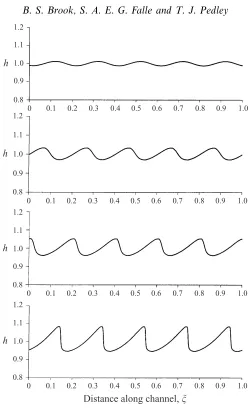
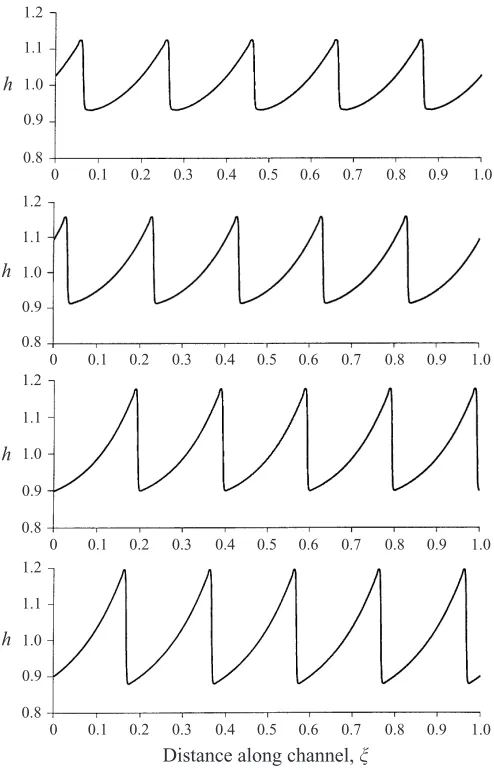
Figure 7.Plots of water height, h, against distance along the channel, ξ. The top panel shows the initial perturbations to the steady uniform flow h = 1 at τ = 0 and the panels underneath show subsequent growth of the perturbations in time (atτ= 0.41, 0.54, 0.71, 0.82, 0.95, 1.19 and 1.8). Solutions are for the parameter values k = 10π, Fo = 2.5, Cf = 0.006, Q= 10 ml s−1 and tanφ=CfFo2.

where

βw=−2Fok+ 2CfL

Fo

ho

i, (6.9)

and

γw= (Fo2−1)k2−3CfL

F2

o

ho

ki. (6.10)

The expression for growth rate can be obtained in a similar manner to that of _§5, and is as follows:

ωI =−CfL

Fo

ho

+1₂˜r1/2sin (1₂θ), (6.11)

Time, τ –5

0 –3

In (amplitude)

–4

0.25 0.75 1.00

–2 –1

0.50

Figure 8. The natural logarithm of the amplitude of the water waves (i.e. ln|h−h∗_{|) against} non-dimensional time, τ, for an initally zero velocity perturbation. Note initial transience for

0< τ <0.15. Compare with figure 9. The solution is for the parameter valuesk= 10π,Fo = 2.5,

Cf= 0.006,Q= 10 ml s−1 and tanφ=CfFo2.

expression for ωR is

ωR=Fok+1₂r˜1/2cos (1₂θ). (6.12) The boundary conditions, as already mentioned, are taken to be periodic and are implemented by first calculating the fluxes in the first and last (nth) computational cells as described in _§3.3. The solution in thenth computational cell is calculated by assuming that cell 1 is to the right of it while the solution in cell 1 is calculated by assuming that the cell nis to the left of it.

The form of the initial condition that is used in the code is that of a sine wave perturbation to the steady solution so that

h(ξ,0) =h∗+_Asin (kξ), (6.13) where_Ais a small initial amplitude andk is a multiple of 2π to be compatible with the boundary conditions. It is important to note that this condition does not of itself prescribe the initial perturbation to the steady fluid velocity, which was at first set to zero. The solutions for water height versus distance down the channels at increasing time steps are shown in figure 7 for k = 10π, Fo = 2.5, Cf = 0.006, Q = 10 cm2s−1 and tanφ=CfFo2.

Figure 8 shows the natural logarithm of the wave amplitude against time for this case. As mentioned above, the graph is expected to be a straight line with gradient

ωI as long as linear theory is valid. As can be seen, there is some transient behaviour before true exponential growth sets in (indicated by the straight section of the curve). The reason for this is that the initial velocity perturbation (zero) is not the solution of the linearized version of (6.3) corresponding to the initial water heighth(equation (6.13)). That solution is

Time, τ –10

0 –6

In (amplitude) _–8

0.5 1.5 2.0

–4

1.0

F_o= 2.0

F_o= 1.5

F_o= 1.0

(b)

Time, τ –4

0 0

In (amplitude)

–1

0.5 1.5 2.0

1

1.0 F_o= 2.5 F_o= 3.0

F_o= 2.25

(a)

–2

–3

Figure 9.The natural logarithm of the amplitude of the water waves against non-dimensional time,

τ, for different steady flow Froude numbersFo>2.0, for an initally non-zero velocity perturbation with (a) k = 2π and (b) k = 10π. See text for details of the velocity perturbation. The solid curve respresents the solution obtained from the numerical code, and the broken lines indicate the corresponding growth rates obtained from the linear stability analysis. The amplitudes in (a) settle down to steady values at approximately 25 s forFo = 2.25, 17 s for Fo = 2.5 and about 10 s for

Fo= 3.0.

When this form of the initial velocity perturbation is adopted, the results, for the same parameter values as figure 8, are shown in figure 9(a). The solid line represents the solution obtained numerically, and the dashed line represents the straight line graph with the gradientωI given by (6.11). As can be seen, the agreement between the numerical and theoretical results is very good now that there is immediate growth and no initial transient. The amplitude graph shows that the exponential growth governed by linear effects ceases at τ_≈0.7 (t_≈12 s) forFo= 2.5, for example, and presumably this is the time at which nonlinear effects begin to dominate. The amplitude growth slows down and, eventually, the amplitude settles down to a constant value.

ζ=λ hn

h_b

hn+1

h_f

ζ

ζ_s

ζ= 0

h_c

h

h_A

h_B

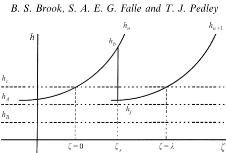
Figure 10.Schematic description of roll wave solutions following Dressler (1949). hA andhB are the solutions of the numerator of (6.20).hC is the critical height through which there is a smooth transition from sub- to supercritical flow. Curves hn and hn+1 are described by equation (6.19). Subscriptsbandfrefer to the maximum and minimum wave heights respectively.

grows and begins to steepen at the wave front. These effects are predicted by the weakly nonlinear analysis (Yu & Kevorkian 1992). Beyond that, once the waves have steepened to form hydraulic jumps, the full nonlinear effects come into play. The evidence for this is the slowing down of the amplitude growth and convergence to a quasi-steady solution in which the roll waves that have evolved out of the initial disturbance move with a constant speed in the positive ξ-direction without further distortion.

Further comparisons are made for different parameter values. The amplitudes are shown in figure 9 with the theoretical graphs superimposed. Agreement between theoretical and numerical results are good both for Fo >2, and for Fo <2 in which case the amplitude decays since ωI is negative. For Fo = 2 we would expect there to be zero-amplitude growth and this is also seen in the numerical solutions.

One further comparison needs to be made for the shallow water case, between the final converged solution in figure 7 and that constructed theoretically by Dressler (1949). The full analysis leading to these roll-wave solutions is described comprehen-sively by Dressler, and we merely summarize his findings here.

Starting from the non-dimensional governing equations (6.3) and (6.4), Dressler sought travelling-wave solutions of the form v(ξ, τ) = v(ζ), h(ξ, τ) = h(ζ), where

ζ =ξ₋cwτ and cw is the speed of propagation of the roll waves. In the continuous section that connects two hydraulic jumps, there must be a smooth transition from sub- to supercritical flow, in the frame of reference of the waves, as sketched in figure 10. Dressler showed that, at this point (ζ = 0 without loss of generality), the variables are given by

vc=

cw

1 +√_G, (6.15)

and

hc= G

c2

w

1 +√_G2

, (6.16)

where

G= Cfc 2

o

ghosinφ

1.2

1.1

1.0

0.9

0.8

0 0.2 0.4 0.6 0.8 1.0

Distance down the channel, ξ

W

ater height,

h

Figure 11.Comparison between the converged roll-wave solution obtained numerically and that constructed by Dressler (1949). The solid curve shows the numerical solution and the broken curve represents the analytical Dressler solution.

The wave speed is related to the flow rateKcin the wave frame by

Kc=hc(cw−vc). (6.18)

The function h(ζ) in the smooth section throughζ= 0 is then given inversely by

ζ = 1

gr

(h₋hc) +

h2

A+hchA+h2c

hA−hB ln

h₋hA

hc−hA

− h

2

B+hchB+h2c

hA−hB ln

h₋hB

hc−hB

,

(6.19)

wherehA, hB are roots of

h2+ (hc− Gc2w)h+Gh

2

c = 0. (6.20)

Finally, the hydraulic jump conditions are used to calculate the values of h in front of and behind the jump, hb and hf, and hence, from (6.19), the positions of the jump relative to ζ = 0. In the calculation it is assumed that the wavelength λ, determined from the wavenumber k of the original small disturbance, is given in advance. Dressler’s model does not explain how a particular wavelength is selected from a random initial disturbance.

0

–2

–4

–6

–8

0 0.025 0.050 0.075 0.100

Time, τ

In (amplitude)

0.125 0.150 Q= 30 ml s–1

k= 4π Q= 40.0 ml s–1

L= 100 cm

Figure 12.The natural logarithm of the amplitude of the perturabation in an inclined collaspible tube (ln_|α₋α∗_{|) against non-dimensional time, τ. Solid curves are the growth rates obtained} numerically and the broken lines represent the growth rates calculated via linear stability analysis. The parameter that has been changed is indicated against each curve. It can be seen that the amplitudes settle down to steady values at different times depending on the parameter values, with a quasi-steady state resulting in about 1.2 s for a flow rate of 40 ml s−1 _{compared with over 3 s for} a flow rate of 30 ml s−1_{. See text for baseline parameters used.}

encouraging, and permits us to ask the same question, of whether roll-wave structures will evolve from an unstable flow, in an inclined collapsible tube.

6.2. Roll waves in inclined collapsible tubes

In order to see what kind of flow can emerge from unstable perturbations in the case of inclined collapsible tubes, we carry out numerical calculations similar to those carried out for the surface waves. To obtain immediate exponential growth, we must choose the initial condition carefully as we have seen. Carrying out the same analysis as for shallow water flow we find that the initial condition has to be of the form

α=α∗+_Aei(kξ−ωτ), (6.21)

and

U=U∗+ ˜rcAei(kξ−ωτ+θc), (6.22) where

˜rceiθc =

ω k −

U∗

α∗ (6.23)

1.2

1.0

0.2

0 0.1 0.2 0.3 0.4

Distance down the tube, ξ α

0.5 0.6 0.8

0.6

0.4

0.7 0.8 0.9 1.0 0.25

0.20

0 0.1 0.2 0.3 0.4

α

0.5 0.6 0.15

0.10

0.05

0.7 0.8 0.9 1.0 0.10

0.09

0.06

0 0.1 0.2 0.3 0.4

α

0.5 0.6 0.08

0.07

0.7 0.8 0.9 1.0 7.9

7.5

0 0.1 0.2 0.3 0.4

α

0.5 0.6 7.8

7.7

7.6

0.7 0.8 0.9 1.0 (×10–1)

Figure 13.Evolution of unstable perturbations to a uniform steady flow in an inclined collapsible tube. Plots are of cross-sectional area,α, against distance down the tube, ξ. The inital condition (τ= 0) is shown by the broken line on the top panel. The solid line on the top panel is the solution at τ= 0.005. Panels underneath show solutions at increasing time (τ= 0.025,0.05,0625) and the final quasi-steady solution is represented by the dashed line on the bottom-most panel (atτ= 0.15).

1.2

1.0

0.2

0

0.06 0.08 0.10

Distance down the tube, ξ

Cross-sectional area,

α

0.8

0.6

0.4

0

0.12 0.14

5 10 15 20 25 30

Speed inde

x,

S=u

/

c

60

50

10

0

0.06 0.08 0.10

Distance down the tube, ξ

Fluid v

elocity

,

u ₄₀

30

20

0

0.12 0.14

5 10 15 20 25 30

W

av

e speed

,

c

(a)

(b)

Figure 14. (a) Cross-sectional area, α, (solid curve) and speed-index, S, (broken curve) against distance down the tube,ξ, for one wavelength. (b) Non-dimensional fluid velocity, u, (solid curve) and wave speed,c, (broken curve) against distance down the tube,ξ, for one wavelength.

40

10

0 0.4 0.8

Cross-sectional area, α

W

av

e speed

,

C

(

α

) 30

20

1.2 1.6

Figure 15.The wave speed functionC(α) against cross-sectional area,α, where

C(α) = (10α10₊3 2α−

3/2₎1/2_.

and the decrease to minimum cross-sectional area together occupy only 10% of the wavelength.

A closer examination of the speed index of the quasi-steady solution shows that there is a smooth transition from sub- to supercritical flow followed by an elastic jump back to subcritical velocity (figure 14a). The unusual double peak in the speed index curve is due to the fact that the wave-speed curve (see figure 15) is not monotonic. For large values ofα, the wave speed is large. As α decreases to α _≈ 0.7, the wave speed decreases as well. Further decrease inαhowever now causes the wave speed to increase again. Now consider figure 14(b). In the region in which the cross-sectional area varies so that there is a smooth transition from sub- to supercritical flow, the area varies from approximately 0.01 to about 1.2. Thus the wave speed decreases (as shown in figure 14b) until the cross-sectional area is _≈ 0.7 at which point the wave speed begins to increase for a short distance until the cross-sectional area is at its maximum at approximately α= 1.2. Then as α decreases from this value, the wave speed decreases too untilα= 0.7 again at which point it once more increases. In the region in which α goes through 0.7 (0.095< ξ < 0.105), the fluid velocity is approximately constant (see figure 14b) and therefore the speed indexS =u/cvaries in the same manner as the wave speed, causing the double peak seen in figure 14(a).

7. Discussion and conclusions

A numerical scheme is developed using the Godunov method and results indicate that this scheme produces stable, accurate solutions to the one-dimensional equa-tions governing unsteady flow in collapsible tubes. Thus further investigaequa-tions into the giraffe jugular vein, as discussed in the introduction, can be carried out with confidence. Such investigations will be reported in a future publication. The fact that non-physical oscillations are no longer a feature of the unsteady solutions also enables us to investigate the evolution of roll-wave-like structures from an initially unstable steady flow. The results show that the numerical solution compares well with that calculated analytically for shallow water waves and that roll waves do emerge out of unstable steady solutions in collapsible tubes.

shallow-water case or the collapsible-tube case is what would determine the wavelength of the roll waves in practice? In all the analyses and computations, of Dressler (1949), Needham & Merkin (1984), Yu & Kevorkian (1992) and of this work, the roll waves of wavelengthλdeveloped from an initial disturbance with prescribed wavelengthλ(= 2π/k), for arbitrary λ. We have performed further computations (for shallow water) in which the initial disturbance consists of two sine waves of different wavelengths (4πand 10π), and either equal amplitudes or with the amplitude of the 4π-wave ten times smaller than that of the 10π-wave. In both cases we found that the eventual roll waves had wavelength 4π, implying that the shorter wavelength necessarily dominates. Presumably this is a consequence of the linear-theory result that the growth rate increases monotonically with k (from (5.21) and (6.11)). Now, a straightforward application of the weakly nonlinear theory of Yu & Kevorkian (1992) can be made to the two-wavelength example. This indicates that, in addition to the steepening of each wave independently, there is a coupling between them which will introduce disturbances with new wavenumbers (the sum and difference of the original two). However, our numerical findings suggest that these are not, eventually, significant. Thus we still cannot say what selects the observed wavelength in experiments.

As far as we are aware there has been only one experimental demonstration of roll waves on inclined collapsible tubes. That was in the MS thesis of Ghandi (1983), who rested a thin-walled, fluid-filled elastic tube on a long inclined surface and adjusted the flow rate so that gravity and friction would balance. He observed periodic waves, presumably roll waves, with wavelengths between 0.1 m and 0.8 m, and propagation speeds somewhat over 1 m s−1_{. The shape of the waves was qualitatively similar to} that constructed by Cowley (1981), rather than those found here, but there was no attempt at quantitative comparison because the tube law was necessarily very different from those assumed here or by Cowley, on account of the dominance of the transverse component of gravity (the tubes were not supported in a bath of liquid, for example). Other experimental attempts to produce collapsible-tube roll waves have been unsuccessful.

We have also found that roll waves do not arise in our simulation of blood flow in the giraffe jugular vein, despite its great length. We suspect that this is a consequence of the specific boundary conditions that we impose, of a given, constant flow rate at the upstream end, leading to supercritical flow, and a given, constant (right atrial) pressure at the downstream end. The boundary conditions for the calculations of §6 were periodic, implying the assumption that the tube is infinitely long. Further investigation into boundary conditions and their effect on the stability criterion is clearly desirable.

This work was done while B. S. B. was a research student of T. J. P. at the University of Leeds; she is grateful to that University for the award of a research studentship. T. J. P. is grateful to the EPSRC for the award of a Senior Fellowship.

Appendix. The nonlinear Riemann solver

The flux vector F_{j−1/2 is the flux at the interface between cell j−1 and cell}

a fully nonlinear solution is necessary because of the highly nonlinear nature of the tube law (equation (2.6)), compared with the corresponding function for the shallow water waves (equation (4.3)).

This Appendix describes the procedure used to obtain a solution to the Riemann problem for the hyperbolic system (3.1), for the vectors (3.4) and (3.5) with the source terms set to zero, and completes the description of the scheme. (The Riemann problem solution procedure that follows is based on an exact solver described by Vanleer 1976.)

The solution procedure requires determination of the three state variables α∗, p∗, and U∗ at the interface. The two conservation laws of mass and momentum are used to calculate the unknowns from the two original statesV_{l = (αl, pl, Ul, Cl) and} V_{r = (αr, pr, Ur, Cr), where}

p= (αF(α)₋Γ), (A 1)

and Γ =Rα

1 F(α) dα.

Recall that each interface is treated as a discontinuity. The state on the left of the interface can be related to the state on the right via the following set of (shock) jump conditions derived directly from the conservative equations (cf. Oates 1975; Cowley 1982)

Ulαl=Urαr = ˜Q, (A 2)

αlUl2+pl =αrUr2+pr. (A 3)

Let us suppose that at the breakup of the discontinuity two waves are formed, one moving off to the right with respect to the fluid, and the other off to the left with respect to the fluid. For the shock/rarefaction on the right we can write a shock relation in the form of (A 2) relating the state at the interface V∗ _{to the state on the} right of the right-moving wave, so that

Wr ₁

αr − 1

α∗

+ (Ur−U∗) = 0, (A 4)

where Wr =| Q˜ |= αr | (s−Ur) | (s is the shock speed relative to the origin) is the mass flux through the shock.

Similarly we can write (A 3) as

Wr(U∗−Ur) =p∗−pr. (A 5)

For a left-moving shock/rarefaction the corresponding expressions are

−Wl ₁

αl − 1

α∗

+ (Ul−U∗) = 0, (A 6)

and

−Wl(U∗−Ul) =p∗−pl. (A 7)

Solving equations (A 5) and (A 7) forp∗ yields

p∗= 1

Wr+Wl

(Wrpl+Wlpr−WlWr(Ur−Ul)), (A 8)

ξ τ

Right shock Left

rarefaction

(c)

ξ τ

Left rarefaction

(d)

Right rarefaction ξ

τ

Right shock

(a)

ξ τ

(b)

Right rarefaction Left

shock

Left shock

Figure 16.ξ, τdiagrams showing the four possible outcomes for initial discontinuous data.

Now the solution to any Riemann problem can be one of the following as shown in figure 16

left shock–right shock left shock–right rarefaction left rarefaction–right shock left rarefaction–right rarefaction.

We consider each wave separately – starting with the right wave.

Right shock

Suppose the right-moving wave is a shock. Then the resolved pressure at the interfacep∗will be greater than the pressurepr on the right of the discontinuity. Thus we use the two shock relations (A 4) and (A 5). Eliminating (U∗₋Ur) yields

Wr=

α∗αr

(p∗₋pr) (α∗_−αr)

1/2

. (A 9)

Right rarefaction

Suppose instead that the right wave is a rarefaction. Then the pressure at the interfacep∗< pr. Now the Riemann invariants along the characteristics dξ/dτ=U±C for these equations are given by

R_± =U_±

Z α

1

C

α dα. (A 10)

we have

Ur− Z αr

1

C

α dα=U

∗₋Z α

∗

1

C

α dα. (A 11)

Eliminating (Ur−U∗) from (A 4) and (A 11) above then yields

Wr=α∗αr Z α∗

1

C α dα−

Z αr 1

C α dα α∗_−α

r

. (A 12)

Note that in the cases of both gas dynamics and shallow water waves, the integrals in the Riemann invariants can be found in closed form and as a result the equivalent expression for (A 12) is much simpler; for instance the corresponding expression for water waves is

Wr=

2h∗_h r √

h∗₊√_hr. (A 13)

In our case the values for the function Rα

1 (C/α) dα are calculated numerically and tabulated.

Exactly similar calculations for the left wave give

Left shock

Wl =

α∗αl (p∗_−p

l) (α∗_−α

l) 1/2

. (A 14)

Left rarefaction

Wl =α∗αl Z α∗

1

C α dα−

Z αl 1

C α dα α∗_−α

l

. (A 15)

To start off the solution procedure we assume that the two waves are shocks. We thus get a reasonable first guess at p∗_=p∗

o by substituting Wr=αrCr and Wl =αlCl into equation (A 8). These approximations toWr and Wl in effect are tangents to the two shock curves at the known points αr and αl. (See figure 17). p∗o is where these straight lines intersect.

The following algorithm is then used to refine the guess:

If p_∗> pr then the right wave is a shock and equation (A 9) is used forWr; if p∗< pr then the right wave is a rarefaction and equation (A 12) is used. If p∗_{> p}

l then the left wave is a shock and (A 14) is used forWl; if p∗_{< p}

l then the left wave is a rarefaction and (A 15) is used.

The updated values of Wr and Wl are then substituted into equation (A 8) to get a new value for p∗ = p∗1. We now use p∗1 to calculate Wl and Wr. The procedure is repeated until p∗_n+1−p∗n is sufficiently ‘small’. The method used here is illustrated graphically in figure 17 and is similar to secant iteration. Once p∗ is determined α∗

is calculated from equation (A 1), U∗ is calculated from equation (A 5) and C∗ is calculated from

C(α) = (10α10+3₂α−3/2)1/2. (A 16) The state at the interface is now determined according to the directions in which the left and right waves move. If (U∗_−C∗_{)>0 and (U}∗_+C∗_{)>0, then the values at the} interface are taken to be the left state; i.e. (α∗_{, U}∗_{, C}∗_{) = (α}

Initial guess (u_r, α_r)

(u_l, α_l)

p*

p*

o p*

l

u

α

Figure 17.The exact solution is the point at which the left and right shock curves intersect,p∗_. The initial guess is shown asp∗

0 and subsequent iterations home in on the exact solution.

ξ τ

U*_–C* (a)

Left rarefaction

U_l–C_l

ξ τ

U*_+C* (b)

Right rarefaction

U_r+C_r

Figure 18.ξ, τdiagrams showing the characteristics of left and right rarefactions spanning the interface.

and (U∗_−C∗_{)<0, then the values at the interface are taken to be the right state; i.e.} (α∗_{, U}∗_{, C}∗_{) = (α}

r, Ur, Cr).

Consider however the possibility that the rarefaction fan spans the interface. In this instance the state at the interface needs to be calculated independently. Suppose the left rarefaction spans the interface as shown in figure 18(a). The head of the rarefaction is given by the left characteristic dξ/dτ = Ul−Cl, and the tail of the rarefaction by the left characteristic dξ/dτ= U∗₋C∗. Thus the condition required for a left rarefaction to span the interface is

Ul−Cl<0< U∗−C∗. (A 17)