Bridge Construction Cost Prediction using Multiple Linear Regression

International Journal of Innovative Technology and Exploring Engineering (IJITEE) ISSN: 2278-3075, Volume-8 Issue-9, July 2019



Abstract: Cost of construction of bridges is predicted using multiple linear regression model, based on data of bridges from Maharashtra state in India. Cost per unit area is taken as an appropriate dependent variable. Using both conventional and double log regression techniques, models for cost/m2 and log of cost/m2 are developed. Total 6 independent variables, which include both qualitative and quantitative variables, are used to develop the model. Height of bridge, average span length and depth of foundation are used as quantitative variables. Zone of construction, deck type and foundation type are used as qualitative variables in developing model. Strength of these independent variables with dependent variable is found out using pearson’s correlation method. Model is then verified using Leave One Out Cross Validation (LOOCV) technique. The most suited regression model obtained from the data experiment is double log regression with R2 of 0.850 and a Mean Absolute Percentage Error (MAPE) of 17.74%, as compared to 25% MAPE observed in past for studies related to traditional cost prediction.

Index Terms: Bridge, Multiple Linear Regression, prediction, construction cost, cost model

I. INTRODUCTION

Infrastructure funding has always been a subject of significant debate and dissonance[1]. Construction clients require early cost estimates to assess the feasibility of the proposed project. Construction contract bid amount forecasting is therefore an important task [2]. The prediction of construction cost is vital for the successful completion of a project, as many planning and execution related decisions depend on predicted cost information [3]. Preliminary cost estimates or feasibility estimates are made before the project’s detailed plans and specifications are known [4] and mainly rely on the conceptual design of the project. Although these forecasts involve very less accuracy and are approximate estimates, they play a significant role in decision making, especially during budgeting, material selection, setting quality standards, timeline of project etc [5]. A cost estimate is a vital component of any construction project. Esimates are also helpful in comparison, financial evaluation of alternative projects, and the application of most suited financing methods [6]. One of the most important components of infrastructure is bridge. The cost of bridges varies with respect to type of foundations, height of structure and specifications adopted [7]. The study here presents method for estimation of cost of bridges in Maharashtra which could be used to work out the

Revised Manuscript Received on July 05, 2019.

Krishna Garkal, Former Post Graduate student, Civil Engineering

Department, College of Engineering, Pune, India.

Dr. N.B. Chaphalkar, Former Associate Professor, Civil Engineering

Department, College of Engineering, Pune, India.

Dr. Sayali Sandbhor, Assistant Professor, Civil Engineering

Department, Symbiosis Institute of Technology, Symbiosis International (Deemed University), Pune, India.

reasonably correct cost in short time. Due to development in infrastructural facilities, bridge construction has increased over the last few years exhibiting substantial cost overruns [5]. Skamris, M.K. and Flyvbjerg, B. [8], found that construction industry faces more than 50% cost overruns as the forecasts used for planning of the work are incorrect by 20–60% compared with actual development. This is a very common scenario in infrastructure projects which is a byproduct of ill forecast during the initial phase of the project. Misleading forecasts may lead to erroneous allocation of funds and project failures in terms of budget. It is thus need of the hour to have an early and accurate estimate of bridge construction project cost [5]. After studying various estimates and present practice of cost estimation for bridges at initial stage, it is observed that Maharashtra requires scientific method for estimation for allocating appropriate funds in the budget. This paper investigates the collected data, develops a model to predict cost using MLR technique and assesses the performance of the model by using LOOCV technique. The study deals with the need to have a ready method of cost estimation beforehand i.e. during early stages of construction or even before the designing phase, in order to carry out feasibility study. This paper proposes a theoretical bridge construction cost estimate method that makes use of data from the past, available for a specific region under study and is based on data of 35 bridges in the state of Maharashtra. The cost estimate method presented herein addresses the bridge cost and applies to three widely used construction methods for foundation.

II. LITERATUREREVIEW

Based on the previous literature pertaining to cost estimation of bridges, it is observed that most research efforts perform computer intensive runs to optimize the final design from technical as well as economic viewpoints via trial-and-error method. Very few studies have been observed to rely on real life structural and economic data of constructed bridges for producing cost estimates [5,9]. There are a number of estimating methods differentiated mainly by the level of precision that is desired in the results [10]. In statistical modeling [11], regression analysis is a statistical process for estimating the relationships among variables. More precisely, regression helps in understanding the relative change in dependent variable with change in independent variables. Lowe D. J., Emsley M. W. and Harding A. [2] studied and used Multiple Regression Analysis (MRA) to predict cost of construction with accuracy of model being R2 as 0.661 and MAPE as 19.3%. Typical traditional estimation methods give accuracy of model with

MAPE up to 25% [2] which

suggests that using

regression analysis, accuracy

Bridge Construction Cost Prediction using

Multiple Linear Regression

of predesigned estimate can increase significantly. Data with large variation in cost can be analyzed effectively by rejecting raw cost as predictor and using its logarithmic form as predictor [12]. Jafarzadeh R. et al. [13] have done robust study on use of MLR for prediction and suggest MLR as simple and robust prediction method for constriction project, they are in favor of using double log regression method for prediction as previously used [2,14]. In Maharashtra, every year, District Schedule of Rates (DSR) is published by government authorities. This DSR provides cost of construction material and man hour required to complete unit work with their rate of wage on per hour basis. Hwang S. [3] presented study to develop dynamic regression model to predict construction cost. He further advocates that cost index is very useful for estimating future cost of construction activities and by knowing trend of cost change, estimator can incorporate cost escalation for budgeting. Construction Cost Index (CCI) was used to make predictive model of cost estimation [3]. Gadage, R. B. [7] used Cost Inflation Index (CII) to bring cost of bridges constructed in previous year on one base year. 26 different bridges in Maharashtra were studied and grouped on basis of their foundation types. Simply by establishing relationship between height of bridge and cost per sq.m, different graphs for each group were generated. Extrapolation of graph helps predict cost of bridge by knowing height and area of deck of bridge. Jafarzadeh R. et al, [13], used LOOCV technique to choose best performing model. In this technique, the researcher compared coefficients of different variables for each different model-generated by keeping one case aside, then he calculated new cost and compared it with the actual cost. The study also recorded values of R and R2 of different models while performing LOOCV, and compared it. Finally, the chosen model was with R2 equals to 0.811, adjusted R2, 0.806 and MAPE of 18.36% for prediction of cost.

III. DATACOLLECTIONANDDATABASE

PREPARATION

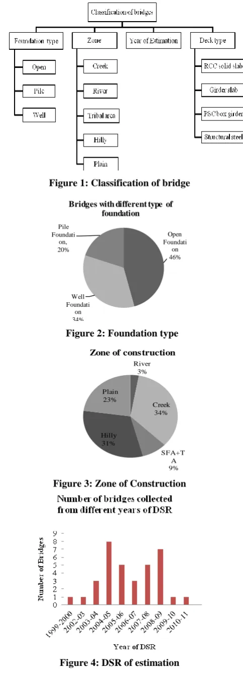
Based on literature, suitable data is found to be the basic requirement for getting good results. Reliability of collected data should also be checked and hence the source of data should be appropriate. For the present study, data was collected from ‘Konkan bhawan’, Belapur, Navi Mumbai. Collected data contains all estimated costs related with bridge construction. This data is then classified as follows to identify variable and assign dummy values for qualitative components within it.

Figure 1: Classification of bridge

Open Foundati

on 46%

Well Foundati

on 34% Pile Foundati

on, 20%

Bridges with different type of foundation

Figure 2: Foundation type

River 3%

Creek 34%

SFA+T A 9% Hilly

31% Plain 23%

Zone of construction

Figure 3: Zone of Construction

International Journal of Innovative Technology and Exploring Engineering (IJITEE) ISSN: 2278-3075, Volume-8 Issue-9, July 2019

RCC Solid slab 28%

Girder Slab 26% PSC

Box Girder 43%

Type of bridge (Deck)

Structural steel deck slab 3%

Figure 5: Superstructure Type Table 1: Dummy variables Type of

Foundation

Dummy Zone Dummy Deck type Dumm y Open

Foundation

1 Hilly/Tribal area

1 Solid Slab 1

Pile Foundation

2 Plain 2 Girder Slab 2

Well Foundation

3 Creek 3 PSC Box 3

River 4 Structural Steel

4

Data is divided into classification as shown in Figure 1. Data comprises of bridges with three types of foundation (Figure 2), open foundation (46%), pile foundation (20%) and well foundation (34%). They are also classified on the basis of zone of construction (Figure 3); 1999 to 2011. Figure 4 gives the classification of data based on the DSR years. Superstructure type (Figure 5) of bridges also affects the cost, hence data is also classified on basis of its deck type. To convert qualitative data to statistical, dummy variables for same are used (Table1). Table 2 gives the set of variables used for regression analysis. Total cost per square meter will be used as independent variable while remaining variables as independent variables.

Table 2: Variables used for analysis

Variable Symbol

Maximum height of structure(RTL) H

Depth of foundation D

Average span Length SL

Deck type S

Foundation type F

Zone Z

Total Cost (Independent variable) C

As we are using log as dependent variable, significance or effect of length and width gets accommodated in single variable. To avoid double inclusion of variables, length and width are not used as independent variable in study.

Log =log (cost) – log ( )

=log (Cost)-log (Length*Width)

=log (Cost)-{Log (Length) +Log (Width)}

Regression Equation,

Log = α + β log + ε; will become

log (cost)= log (Length)+log (Width) +α + β log + ε

A. Data Conversion- Converting Cost Using Cost Inflation Index (CII)

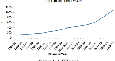
In case of accuracy of prediction, long-term predictions can be more prone to errors. Forecast errors become larger as prediction period becomes longer. If index values are used, the models are observed to respond quickly thereby allowing a quick adjustment to existing prediction (Hwang S., 2009). CII is published every year by Income Tax (IT) Department, Government of India (Figure 6). By comparing CII of different years it becomes possible to change cost to any particular reference year.

Figure 6: CII Trend

To calculate updated cost of bridges, CII method is used. For updating cost, financial year 2015-2016 is taken as referenced year, hence all costs are updated to financial year 2015-2016 using the following relations.

Dynamic cost=CII Factor × Original cost

Where,

B. Data Conversion- Cost Conversion as Per Zone

Cost of bridges constructed in special zones are identified and their costs are normalized by reducing it to required percentage according to District Schedule of Rates (DSR). For different types of areas, an increase of percentages over the normal schedule of rates (basic completed item rates) is prescribed as follows:

Corporation Areas - 5% Sugarcane factory area (within 10 Km. radius) -5% Notified Tribal Areas- 10% Notified Hilly / Inaccessible areas- 10% Inside Premises of Central Jail, Mental Hospital, Raj Bhavan,

Prison- 15%

Collected data comprises of many bridges constructed in Hilly, Notified Tribal Area.

C. Data Conversion- Logarithm in Regression

Using the logarithm of variables helps in making the effective relationship non-linear, while maintaining the linearity. For non-linear relationships between dependent and independent variables, transforming variables logarithmically is a very effective practice [15]. Logarithmic transformations are also a convenient means of transforming a highly skewed variable into one that is more approximately normal. In fact, there is a distribution called the log-normal distribution defined as a distribution whose logarithm is normally distributed but whose untransformed scale is skewed [16].

Linear model:

Linear-log model: Y = α + β log + Log-linear model: Log Y = α + β + Log-log model: Log Y = α + β log + ε

In occurrences where both dependent and independent variables are log-transformed, the interpretation is a combination of the linear-log and log-linear cases above. Here linear and log-log models are developed for prediction of cost of bridge.

IV. MODELPREPARATION

The p-value approach involves determining "likely" or "unlikely" by determining the probability assuming the null hypothesis were true, of observing a more extreme test statistic in the direction of the alternative hypothesis than the one observed [17]. A small p-value (≤ 0.05) indicates strong evidence against the null hypothesis, so it is rejected [18]. The bivariate Pearson Correlation [19] produces a sample correlation coefficient, r, that measures the strength and direction of linear relationships between pairs of continuous variables. Correlation can assume any value in the range -1 to 1 where the sign represents the direction of the relation and the r value represents the strength of the correlation (IBM, 2016), where r between 0.1 to 0.3 represents weak correlation, 0.3 to 0.5 represents moderate correlation and greater than 0.5 represents strong correlation. Table 3 & 4, shows values of r and p indicating relationship between variables increases when taken in their logarithmic form. As all variables shows moderate to strong relationship with independent variable, regression analysis can be done.

Table 3: Correlation Sr.

no.

Variable (in

unlogged form) Symbol “r”

value Strength “p” value

Signif icance

1 Maximum height of

structure (RTL) H 0.598 Strong 0 <0.05 2 Depth of foundation D 0.755 Strong 0 <0.05

3 Average span

Length SL 0.665 Strong 0 <0.05 4 Deck type S 0.632 Strong 0 <0.05 5 Foundation type F 0.656 Strong 0 <0.05

6 Zone Z 0.451 Moderat

e 0.01 <0.05

7 Total Cost C - - - -

Table 4: Correlation (in Ln)

A. Application of MLR

a) Model 1: Conventional Regression

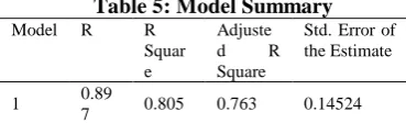
A total of 35 bridges are selected for developing MLR models. Given that six predictors are considered in this study, development of total 26 regression models is possible and examination of all models is practically infeasible. In this study, the p value for selecting predictors was set (p < 0.005) to allow whole model to be developed using the “Enter” technique (Jafarzadeh R. et al, 2014). Firstly, whole data is used to run regression. All predictors like Height of Bridge (H), Depth of Foundation (D), Avg. Span length (SL) are used with their original values; whereas Zone of Construction (Z), Foundation Type (F), Deck Type (D) are used as dummy variables to develop the model. After forcefully entering all variables (Enter Technique) in regression analysis it gives results as from Table 5.

Table 5: Model Summary Model R R

Squar e

Adjuste

d R

Square

Std. Error of the Estimate

1 0.89

7 0.805 0.763 0.14524

Model summary shows good result in favour of regression. R value 0.897 indicates that the model is strong; whereas R2 0.805 means model fitting is good, with standard error of 0.014524. Table 6 generated after regression analysis, gives coefficient for different variables along with constant, which is Y intercept, conceptually, of regression line. Now using this coefficient one can predict value for bridge using following formula:

Predicted Value=

-0.35+0.025*H+0.014*D-0.008*SL+0.094*Z+0.040*S+0.0 86*F.

Table 6: Coefficient values Model 1 Unstandardized Coefficients

B Std. Error (Constant) -0.035 0.092

H 0.025 0.006

D 0.014 0.004

SL -0.008 0.006

Z 0.094 0.041

S 0.04 0.089

F 0.086 0.038

Table 7 presents short summary of result. The model has R2 of 0.897, with MEP=5.7% and MAPE=17.74%. Figure 7 shows relation of predicted cost

with actual cost generating approximately 450 line which is good indication for

Sr. no

Variable (in

unlogged form) Symbol “r”

value Strength “p” valu e

Signifi cance

1 Maximum height of

structure(RTL) H 0.665 Strong 0 <0.05 2 Depth of foundation D 0.838 Strong 0 <0.05 3 Average span

Length SL 0.731 Strong 0 <0.05

4 Deck type S 0.676 Strong 0 <0.05 5 Foundation type F 0.565 Strong 0 <0.05

6 Zone Z 0.473 Moderate 0 <0.05

International Journal of Innovative Technology and Exploring Engineering (IJITEE) ISSN: 2278-3075, Volume-8 Issue-9, July 2019

accuracy of model. Residual distribution is a measure of accuracy by visualization. All points are concentrating towards zero (Figure 8) which is one of indication that the model is good and not overfitted. This graph is drawn with predicted cost against its error.

Table 7: Result Summary Parameters Regression

R 0.897

R2 0.805

Adj. R2 0.763

Std. Error 0.14524 Mean percentage

Error 5.73%

MAPE 17.74%

Variables entered H D SL S F Z Variables excluded -

Upper outlier 0.64 Lower outlier -0.32

Figure 7: Predicted cost (Model 1)

Figure 8: Residual distribution (Model 1) b) Model 2: Logarithmic Regression

Same group of 35 bridges is selected for developing MLR model as in [13]. This is same model as model 1, only difference is double log regression has been used for running regression. Six predictors are considered in this model. Dependent variable (Cost/m2) and predictors-both are used in their logarithmic form. In this model as well, the p value for selecting predictors was set (p < 0.005). At first, whole data was used to run regression. All predictors- Height of Bridge (H), Depth of Foundation (D), Avg Span length (SL) are used with their logarithmic values; whereas Zone of Construction (Z), Foundation Type (F), Deck Type (D)- these variables used as dummy variables in logarithmic form to develop model. Table 8 gives regression results that show good result in favor of regression. R value is 0.928, which is comparatively higher than previous model (0.897) indicating the model is very strong; whereas R2 is 0.833, which is also significantly higher than that of previous model (0.805).This

clearly shows that model fitting is good, with standard error of 0.20666.

Table 8: Model 2 summary

Model R R Square Adjusted R

Square

Std. Error of the Estimate

2 0.928 0.862 0.833 0.2067

Table 9 generated after regression analysis, gives coefficient for different variables with constant, which is Y intercept, conceptually, of regression line. Now using this coefficient one can predict value for bridge using following formula:

Predicted value =

-1.466+0.549*LnH+0.394*LnD0.515*LnSL+0.246*LnZ+0. 263*LnS+0.128*LnF

Table 9: Coefficient (Logarithmic) Model 2 Unstandardized

Coefficients B Std. Error (Constant) -1.466 0.379

LnH 0.549 0.112

LnD 0.394 0.077

LnSL -0.515 0.241

LnZ 0.246 0.092

LnS 0.263 0.284

LnF 0.128 0.093

All these predictors are in their logarithmic form; hence predicted value also gets in logarithmic form. By using exponential of this value, actual predicted value is generated as follows;

Actual Predicted value Cp=

e(-1.466+0.549*LnH+0.394*LnD0.515*LnSL+0.246*LnZ+ 0.263*LnS+0.128*LnF)

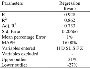
Table 10 Result summary (Logarithmic)

Parameters Regression

Result

R 0.928

R2 0.862

Adj. R2 _0.733

Std. Error 0.20666

Mean percentage Error 1%

MAPE 16.00%

Variables entered H D SL S F Z Variables excluded -

Upper outlier 31%

Lower outlier -27%

Figure 9: Predicted cost (Model 2)

Figure 10: Residual distribution (Model 2) B. Validation for Model

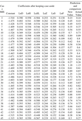
Validating and cross-checking of estimates is an important step, that is sometimes overlooked. Leave-one-out cross validation is carried out to validate model in which the function generator is trained on all the data except for one case and a prediction is made for that case. As before, the error is computed and used to evaluate the model. The evaluation given by LOOCV is good, but it is very expensive to compute. Each time by keeping one case aside regression is performed which gives values of various parameters of regression like R, R2, Adj. R2. There is no significant change in values of parameters. After performing total 35 regressions by keeping one case aside, each time, new constants and coefficients are obtained which are recorded in Table 11.

Table 11: LOOCV coefficients and predicted value

There is no much variation in new constants and coefficients. Using the combination of any set of constant and coefficients, cost for bridge can be predicted. Using the given set of constant and coefficients, cost for the case kept aside is predicted and compared with actual predicted cost for model 2 (Table 11). From above results, it can be observed that the model is strong enough to predict cost for bridges of all types. Prediction error as given by the model shows that total 25 out of 35 bridges were predicted within absolute error of 5% and all 35 out of 35 bridges were predicted within absolute error of 10%.

V. CONCLUSION

It is found that log-log regression method yields better results than that of conventional regression. Comparison of Table 7 and Table 10 for the performance of both conventional and log-log regression method clearly shows better result yielding capacity of log-log regression. MAPE and MEP value of conventional regression are significantly reduced in log-log regression. Error in prediction using conventional method (Model 1) is 18% and double log regression (Model 2) method predicts cost with absolute error of 16%. Here total 2% of error is minimized by using double log method for regression. Also in MEP

substantial reduction of error is recorded i.e. from 6% to 1%. In same way, it is Cas

e MIS

Coefficients after keeping case aside

Prediction and comparison

Constant LnD LnH LnSL LnZ LnS LnF New Value

International Journal of Innovative Technology and Exploring Engineering (IJITEE) ISSN: 2278-3075, Volume-8 Issue-9, July 2019

observed that all models with logarithmic form give better prediction with minimum error. It is thus concluded that model based on double log regression performs well than conventional regression to predict cost of bridges. It can be observed that error in prediction of cost for case which was skipped in LOOCV, is within 15% for 99 % of cases. So this validates results obtained by using double log regression method. For cost prediction one can use formula subject to absolute error of 16%

Cp= e (-1.466+0.549*LnH+0.394*LnD0.515*LnSL+

0.246*LnZ+0.263*LnS+0.128*LnF)

There is scope to develop new software, where large database can be prepared and stored for analysis. After analyzing data with additional database, the model would minimize the error and would give more accurate predictions. For study, estimations taken into account are based on DSR of that particular district. DSR changes from district to district. Hence there is no uniformity in estimation as cost of some construction material, say sand, will not be same in different districts. Hence, there is always scope for error when directly comparing estimation of bridges from different districts of the state.

REFERENCES

1. Hollar D. A., Rasdorf W., Hummer J. E., Arocho I., and Hsiang S.M. (2013). “Preliminary Engineering Cost Estimation Model for Bridge Projects”, Journal of Construction Engineering and Management, 10.1061/ (ASCE) CO.1943-7862.0000668, 1259-1267.

2. Lowe D. J., Emsley M. W. and Harding A. (2006). “Predicting Construction Cost Using Multiple Regression Techniques” Journal of Construction Engineering and Management 10.1061(ASCE) 07339364(2006)132:7(750), 750-758.

3. Hwang S. (2009). “Dynamic Regression Models for Prediction of Construction Costs”, Journal of Construction Engineering and Management, 10.1061/ASCECO.1943-7862.0000006, 360-367. 4. Flyvbjerg B., Holm M.S., and Buhl S. (2002), "Underestimating Costs

in Public Works Projects: Error or Lie?" Journal of the American Planning Association, vol. 68, no. 3, 279-295.

5. Fragkakis N., Lambropoulos S. and Pantouvakis J.P. (2010). “A Cost Estimate Method for Bridge Superstructures Using Regression Analysis and Bootstrap” International Journal of Organization, Technology and Management in Construction, 182-190.

6. Project Cost Estimating Guidelines, Version 01.02 September 30, 2013, Ministry of Transportation and Infrastructure http://www.th.gov.bc.ca/gwwpmss/Content/costestimating.asp, http://www.th.gov.bc.ca/publications/planning/guidelines/cost_estimat ing_guidance.pdf (Accessed on: 10/06/2016)

7. Gadage, R. B. (2015). “Innovative Method for Estimation of Bridge Designs”

Journal of the Indian Roads Congress, Volume 2, 165-168.

8. Skamris, M.K. and Flyvbjerg, B. (1997), “Inaccuracy of traffic forecasts and cost estimates on large transport projects”, Transport Policy, Vol. 4 No. 3, pp. 141-146.

9. Antoniou F., Konstantinidis D., Aretoulis G., Xenidis Y (2017). Preliminary construction cost estimates for motorway underpass bridges, International Journal of Construction Management, Vol 18, No. 4: Research-based directions for future engineering and construction, pp. 321-330.

10. Challal A. and Tkiouat M. (2012). “The Design of Cost Estimating Model of Construction Project: Application and Simulation”, Open Journal of Accounting, dx.doi.org/10.4236/ojacct.2012.11003, 15-26 11. Gaccione P. and Blanchard M.S. (2008). “Nonlinear Mixed Effects

Models, a Tool for Analyzing Repeated Measurements; A Brief Tutorial

Using SAS Software.”

http://ssc.utexas.edu/docs/sashelp/sugi/23/Stats/p228.pdf (May 17,2016)

12. Behmardi B., Doolen T. and Winston H. (2013). “Comparison of Predictive Cost Models for BridgeReplacement Projects” Journal of

Construction Engineering and Management, 10.1061/ (ASCE) ME.1943-5479.0000269, 04014058.

13. Jafarzadeh R., Ingham J. M., Walsh K. Q., Hassani N. and Ghodrati G. R. (2014). “Using Statistical Regression Analysis to Establish Construction Cost Models for Seismic Retrofit of Confined Masonry Buildings” Journal of Construction Engineering and Management, 10.1061(ASCE) CO.1943-7862.0000968, 04014098.

14. Williams, T. P. (2003). “Predicting final cost for competitively bid construction projects using regression models.” International Journal of Project Management, 21(8), 593–599.

15. Strine R. (2001). “Logs Transformation in a Regression Equation” Statistics 221, 148-151.

16. Benoit K., “Linear Regression Models with Logarithmic Transformations Methodology” Institute London School of Economics

[email protected] March 17, 2011

http://www.kenbenoit.net/courses/ME104/logmodels2.pdf(10/06/16) 17. Rosenberger J (2016) Review of Basic Statistical Concepts, Online

course, Department of Statistics , Pennstate Eberly College of science. https://onlinecourses.science.psu.edu/statprogram/node/138 (Accessed on: 10/06/2016)

18. IBM (2016), SPSS 20.0 [Computer software]. Pune, IBM. http://ibm-spss-statistics.soft32.com/( Accessed on: 02/08/2016)

19. Kent State University (2016),

http://libguides.library.kent.edu/SPSS/PearsonCorr (Accessed on: 10/06/2016)

AUTHORSPROFILE

Krishna Garkal has completed masters in construction

and management, civil engineering from college of engineering pune. This work is the compilation of dissertation work conducted by him as a partial fulfilment of his master’s degree.

Dr. Nitin B. Chaphalkar is an associate professor at department of civil engineering, college of engineerign pune with an experience of more than 22 years in teaching. He has obtained his phd. From iit, delhi and has area of expertise in legal aspects in construction, construction management, use of artificial intelligence in civil engineering.

Dr. Sayali Sandbhor Is An Assistant Professor At