Three decades of simulated global terrestrial carbon fluxes from a data assimilation system confronted with different periods of observations

https://doi.org/10.5194/bg-16-3009-2019 © Author(s) 2019. This work is distributed under the Creative Commons Attribution 4.0 License.

Three decades of simulated global terrestrial carbon fluxes

from a data assimilation system confronted with different

periods of observations

Karel Castro-Morales1,a, Gregor Schürmann1, Christoph Köstler1, Christian Rödenbeck1, Martin Heimann1,3, and Sönke Zaehle1,2

1_{Max Planck Institute for Biogeochemistry, Jena, Germany}

2_{Michael Stifel Center Jena for Data-Driven and Simulation Science, Jena, Germany}

3_{Institute for Atmospheric and Earth System Research, Faculty of Science, University of Helsinki, Helsinki, Finland} a_{now at: Institute of Biodiversity, Aquatic Geomicrobiology, Friedrich Schiller University, Jena, Germany}

Correspondence:Karel Castro-Morales ([email protected]) Received: 19 December 2018 – Discussion started: 2 January 2019

Revised: 5 June 2019 – Accepted: 28 June 2019 – Published: 8 August 2019

Abstract. During the last decade, carbon cycle data assim-ilation systems (CCDAS) have focused on improving the simulation of seasonal and mean global carbon fluxes over a few years by simultaneous assimilation of multiple data streams. However, the ability of a CCDAS to predict longer-term trends and variability of the global carbon cycle and the constraint provided by the observations have not yet been as-sessed. Here, we evaluate two near-decade-long assimilation experiments of the Max Planck Institute – Carbon Cycle Data Assimilation System (MPI-CCDAS v1) using spaceborne es-timates of the fraction of absorbed photosynthetic active ra-diation (FAPAR) and atmospheric CO2concentrations from

the global network of flask measurement sites from either 1982 to 1990 or 1990 to 2000. We contrast these simulations with independent observations from the period 1982–2010, as well as a third MPI-CCDAS assimilation run using data from the full 1982–2010 period, and an atmospheric inver-sion covering the same data and time. With 30 years of data, MPI-CCDAS is capable of representing land uptake to a suf-ficient degree to make it compatible with the atmospheric CO2record. The long-term trend and seasonal amplitude of

atmospheric CO2concentrations at station level over the

pe-riod 1982 to 2010 is considerably improved after assimilating only the first decade (1982–1990) of observations. After 15– 19 years of prognostic simulation, the simulated CO2

mix-ing ratio in 2007–2010 diverges by only 2±1.3 ppm from the observations, the atmospheric inversion, and the MPI-CCDAS assimilation run using observations from the full

pe-riod. The long-term trend, phenological seasonality, and in-terannual variability (IAV) of FAPAR in the Northern Hemi-sphere over the last 1 to 2 decades after the assimilation were also improved. Despite imperfections in the representation of the IAV in atmospheric CO2, model–data fusion for a decade

of data can already contribute to the prognostic capacity of land carbon cycle models at relevant timescales.

1 Introduction

The observed contemporary increase in atmospheric CO2is

driven by anthropogenic emissions from fossil fuels, land use change (2007–2016 average: 11.1±0.6 GtC yr−1), and the concurrent net carbon uptake of the ocean and land from the atmosphere, which take up approximately 22.4 % and 28 % of the anthropogenic flux, respectively. Despite recent ad-vances in atmospheric observations and ocean and land mod-eling, there is an imbalance of 5.6 % (0.6 GtC yr−1_{) between}

the ocean and land sinks, carbon emissions, and changes in the atmospheric CO2concentration (Le Quéré et al., 2018).

and dynamics of the global terrestrial carbon cycle across dif-ferent temporal scales, and their contribution to the global carbon cycle, is challenging because the substantial hetero-geneity and complexity in land ecosystems and challenges in the quantification of contemporary effects and response of these ecosystems to increasing postindustrial CO2

concentra-tions (Lienert and Joos, 2018; Stocker et al., 2014; Wang et al., 2017).

One strategy to reduce the mismatch between carbon flux predictions from land surface models and measured at-mospheric CO2concentrations is through data assimilation

(DA) techniques, meaning to “train” the land models by con-fronting them systematically with observations of carbon-related variables (Raupach et al., 2005). During DA, pro-cess parameters of land surface models are adjusted through numerical minimization techniques to reduce the misfit be-tween model results and actual observations under consid-eration of the statistical properties of both data sets. While atmospheric transport inversions are a method used to in-fer the sinks and sources of CO2 between the atmosphere

and land, or ocean, from atmospheric CO2 measurements

(Newsam and Enting, 1988; Peylin et al., 2013; Rayner et al., 1999; Rödenbeck et al., 2003), the application of car-bon cycle data assimilation systems (CCDASs) provides ad-ditional opportunities. In CCDAS, the process-based carbon cycle mechanisms in land surface models are informed with measurements to support a better estimate of the terrestrial carbon cycle, and improve the capacity to project its dynam-ics. With this purpose, several CCDASs have been devel-oped in the past (e.g., Kaminski et al., 2012, 2013; Lienert and Joos, 2018; Peylin et al., 2016; Scholze et al., 2016). The difference among some of these models is the varia-tional or sequential statistical approach they follow during the data assimilation process (Montzka et al., 2012). A com-mon characteristic in these models is their capacity for inte-grating long-term and time-consistent globally available ob-servational records related to the carbon cycle such as atmo-spheric CO2 measurements from flask and in situ networks

(Conway et al., 1994), as well as remote-sensing products of canopy phenology properties such as MODIS NDVI (Mod-erate Resolution Imaging Spectroradiometer – Normalized Difference Vegetation Index) (Rouse et al., 1974) and FA-PAR (Disney et al., 2016; Pinty et al., 2011a).

Previous studies have analyzed the prognostic capability of the data assimilation systems (e.g., Rayner et al., 2011, 2005; Scholze et al., 2007; Schürmann et al., 2016), but only for a few years of prognosis after the assimilation. Scholze et al. (2007) concluded that the CCDAS built around BETHY (Biosphere Energy Transfer Hydrology) is capable of pro-viding a prognostic period of 4 years (2000–2003) of at-mospheric CO2after data assimilation of 21 years (1979 to

1999) of CO2concentrations. Schürmann et al. (2016)

dis-cussed the prognosis capability of the Max Planck Institute – Carbon Cycle Data Assimilation System (MPI-CCDAS v1) for 2 years after a short assimilation period of 5 years. Rayner

et al. (2011) showed that the uncertainty related to model pa-rameters during the prediction of CO2fluxes with a CCDAS

is considerably reduced when the model parameters are con-strained with 2 decades of atmospheric measurements; how-ever, these results were obtained with a model that ignores the interacting effects of water, energy, and phenology on the carbon cycle predictions.

The overarching aim of this work is to understand the abil-ity of the MPI-CCDAS v1 to make decadal projections of the land C cycle when the assimilation is confronted with dif-ferent temporal windows from two observational constraints: FAPAR from remote-sensing data and atmospheric CO2

con-centrations from the global flask measurement network. For this, we present 3 decades of modeled land carbon fluxes with the MPI-CCDAS and investigate the effect of withhold-ing information from recent decades in the projected carbon fluxes and the ability of the model to reproduce the observa-tions during the period of data assimilation. We also analyze trends and seasonal variations in the simulated signals during the periods of the assimilation and compare to independent results to evaluate the model performance. With these results, we gain insights into the number of observations (in terms of decadal scale) necessary in data assimilation systems to im-prove the representation of the global terrestrial carbon cycle components. These results open the possibility of including newly measured data in CCDAS that are only available for periods of less than a decade.

2 Methods 2.1 MPI-CCDAS

The MPI-CCDAS was built around the Jena Scheme Biosphere-Atmosphere Coupling in Hamburg (JSBACH) land surface model (Dalmonech and Zaehle, 2013; Raddatz et al., 2007; Reick et al., 2013) and follows a variational ap-proach that simultaneously reduces the model–data misfit for multiple independent carbon cycle data sets (Kaminski et al., 2013). Since its first development based on the BETHY – CCDAS, the MPI-CCDAS has undergone several code mod-ifications and improvements, as well as tests of the assimi-lation of new observational data sets (e.g., Kaminski et al., 2012, 2013; Rayner et al., 2005; Scholze et al., 2016; Schür-mann et al., 2016), with the aim of further improving the representation of land carbon fluxes. The history of the MPI-CCDAS and other current MPI-CCDASs is extensively discussed in Scholze et al. (2017).

this work. Furthermore, previous evidence has shown that a higher spatial resolution in global vegetation models does not exert a considerable influence in the simulated carbon fluxes at global or regional scales when compared to results ob-tained with a coarse grid (Müller and Lucht, 2007). The lack of influence to improve the simulated global C fluxes due to changes in the model spatial resolution might also apply to CCDAS (Peylin et al., 2016).

The spatial distribution of the different plant functional types (PFTs) in JSBACH is shown in Fig. S1 (Supplement). The selected parameters for the assimilation procedure and their prior and range of values were based on Schürmann et al. (2016), where an extensive sensitivity study led to retain-ing those parameters with a substantial effect on the sim-ulated carbon and water fluxes, as well as on phenology. The majority of the selected parameters for the optimiza-tion are linked to phenology, but there are also parameters related to photosynthesis and global parameters that control the land carbon turnover during the assimilation. The final list of parameters together with their initial value obtained from an independent forward simulation of JSBACH 3.0 (see Sect. 2.3.1) are shown in Table 1.

The MPI-CCDAS starts with an initial guess for the model control vector (p_pr) of carbon cycle properties, model states, and their Gaussian uncertainty (“prior”) with covarianceCpr.

The model control vectorpis iteratively updated to minimize a joint cost functionJ (Eq. 1) describing the misfit between observational data streams (d; FAPAR and atmospheric CO2,

both with covariance Cd) and the corresponding simulated observation operators of the MPI-CCDASM(p), taking into account the uncertainties in the observational data assuming a Gaussian distribution and the information from the prior.

J (p)= 1

2(M (p)−d) T_C−1

d (M (p)−d)

+ p−p_prTC_pr−1 p−p_pr (1)

During the optimization procedure, a new model trajectory is determined in each iteration (i.e., in every cycle when the model recalculates the cost function for the difference between the model parameters and the observational con-straint), such that energy and mass are conserved through the entire assimilation window (Kaminski and Mathieu, 2017). The gradient of the cost function with respect to the model control vector (∂J_∂p) is evaluated with a tangent-linear ver-sion of JSBACH 3.0, which was generated through automatic differentiation using a TAF (transformation of algorithms in Fortran) compiler tool (Giering and Kaminski, 1998). With this tangent-linear version of the model code, the derivatives for the parts of the model code whereJ (p)is evaluated (i.e., code parts that depend on the control variables) are accu-rately calculated following the chain rule of calculus. Thus, the mathematical formulation of the code involved in the cost function must be differentiable. Since this was not the case for the phenological code of JSBACH 3.0, the phenology

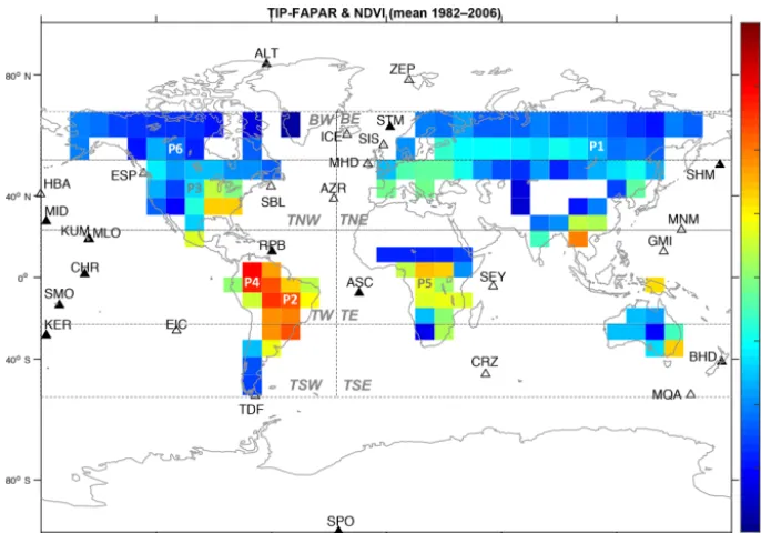
Figure 1.Global distribution of the temporal mean (1982–2006) of the merged satellite FAPAR product used in the assimilation procedure. It also shows the spatial coverage of eight regions globally distributed: boreal west and east (BW and BE, for latitudes north of 60◦N), temperate northwest and northeast (TNW and TNE, between latitudes 20 and 60◦N); tropical west and east (TW and TE, between latitudes 20◦N and 20◦S); temperate southwest and southeast (TSW and TSE, for latitudes south of 20◦S). Also shown are the six selected pixels: P1, for the coniferous deciduous (CD) phenotype in the East Siberian Taiga; P2, for the C4pastures, and grasses (TrH) of central Brazil;

P3, for the C3 and C4crops, pastures and grasses (TeCr and TeH) of the northern USA; P4 and P5, for tropical evergreen trees (TrBe)

situated in northwestern Brazil and central Africa; and P6, for coniferous evergreen (CE) located in Canada. The location of 28 stations of the CO2network measurements (filled triangles, stations only included in DEC1; empty triangles, stations included also in ALL and DEC2)

for analysis of the assimilation results are also included.

scheme was updated following Knorr et al. (2010), where the minimum and maximum calculations in the entire code were replaced by smoothing functions to avoid abrupt transitions (Schürmann et al., 2016).

2.2 Observational data sets 2.2.1 FAPAR

The fraction of the radiation that is absorbed by plants dur-ing photosynthesis (FAPAR) is a component of the land sur-face radiation budget that dynamically indicates the status of the vegetation canopy over space and time (Gobron et al., 2006). In a previous study, MPI-CCDAS was constrained by MODIS TIP (Two-Stream Inversion Package) FAPAR (here-after TIP-FAPAR) generated from the inversion of a 1-D ra-diation transfer model (Pinty et al., 2006, 2007) using the MODIS broadband visible and near-infrared spectral white sky surface albedo as input (Clerici et al., 2010; Pinty et al., 2011a, b). For this study, the TIP-FAPAR product was avail-able only from 2003 to 2011, making it unsuitavail-able for the indented longer assimilation period. While there are long-term remotely sensed proxies of FAPAR, such as the NDVI (Rouse et al., 1974), it has been found previously that NDVI

was less reliable than TIP-FAPAR in terms of the seasonal cycle amplitude of vegetation seasonality (Dalmonech and Zaehle, 2013; Dalmonech et al., 2015). Therefore, we used as FAPAR proxy the Global Inventory Monitoring and Mod-eling System (GIMMS) NDVI product for the period 1982 to 2006 (Tucker et al., 2005), and merged it with the TIP-FAPAR product to provide a longer record of vegetation greenness. The maximum and minimum NDVI values were rescaled at the pixel level to coincide with those from the TIP-FAPAR for the overlapping periods (i.e., 2003 to 2006) following

FAPARmod=

NDVI−NDVImin,x NDVImax,x−NDVImin,x

× TIPmax,x−TIPmin,x+TIPmin,x, (2) wherex is the period from 2003 to 2006 for each data set, and NDVI is the full NDVI product from 1982 to 2006, with minimum values given by NDVIminand maximum values by

NDVImax. TIPmin and TIPmax are the corresponding

un-certainty of the available TIP-FAPAR data was considered to be the uncertainty for the entire time series. Due to a tech-nical failure in the MPI-CCDAS, the final FAPARmod

prod-uct used in the assimilation procedure only spans from 1982 to 2006 and the last 4 years from the TIP-FAPAR product were not considered. For this study, this product was aggre-gated to match the model grid horizontal resolution consider-ing background snow-free and snow-covered conditions sep-arately (Schürmann et al., 2016).

To discard pixels in the global FAPAR data that might lead to bias during the assimilation procedure, we applied a mask to the global FAPAR grid following three criteria. (1) We masked out the grid cells with crop-dominating phenology of >20 % since no explicit crop phenology is described in JSBACH. This step has consequences in areas where other relevant functional types are also present in the same grid cells, such as deciduous broadleaves that are also abundant in the USA and Europe. As a result, the parameters related to deciduous broadleaves are constrained from other loca-tions; (2) we further masked out pixels that hold a low corre-lation (R2<0.2) when the prior model results are compared to the observations, as we had previously found that the MPI-CCDAS is incapable of correcting such poor model behav-iors (Schürmann et al., 2016). Finally, (3) we masked out pix-els located in areas where phenology abundance is low, i.e., deserts, because they would influence the optimization caus-ing significant bias due to global compensatcaus-ing effects. The final FAPAR product used during the assimilation contains 40 % of the original number of pixels after the applied mask, resulting in more pixels distributed in the Northern Hemi-sphere compared to the southern areas. These observational data will be referred to hereafter as FAPARobs (see Fig. 1

for the global distribution of mean FAPARobsfrom 1982 to

2006).

2.2.2 Atmospheric CO2concentrations and

observation operator

Measurements of atmospheric CO2mixing ratios were taken

from the flask data continuous record of 28 sites in the NOAA CMDL station network (Conway et al., 1994; Röden-beck et al., 2003). The selection criteria included the length of the record (on average 19 years) (Fig. A1 in Appendix A) and focused on remote and ocean stations with low impact of local carbon sources and sinks of carbon (Schürmann et al., 2016) (see the location of CO2 stations in Fig. 1). In

the MPI-CCDAS, the atmospheric transport of CO2is

cal-culated by integrating the simulated half-hourly net CO2

fluxes to monthly values followed by the transport calcu-lation with the Jacobian representation of the atmospheric transport model TM3 that is driven with meteorology fields from NCEP (National Centers for Environmental Prediction) reanalysis (Heimann and Körner, 2003; Rödenbeck et al., 2003). During the generation of the monthly transport ma-trices, the precise sampling time of flask measurements as

well as the 3-hourly atmospheric transport was considered to minimize the representation error due to short-term fluctu-ations in atmospheric transport and to minimize the impact of synoptic atmospheric transport variability on the simu-lated seasonal and long-term dynamics of atmospheric CO2

at the monitoring stations. Through this approach, the non-linear effect of weather anomalies on the surface fluxes were also taken into account. TM3 runs at horizontal “fine grid” (fg) resolution of 4◦×5◦. Due to computational demands, it is not possible at this stage to use the MPI-CCDAS at the same fine grid resolution as in the TM3. The treatment of uncertainties is performed in the same way as in the TM3 at-mospheric inversion (Rödenbeck et al., 2003) but imposing a floor value of 1 ppm on the uncertainties (Rayner et al., 2005) to allow a range for the comparison to the observational op-erator.

We also compare the fluxes from the assimilation to fluxes obtained from an atmospheric transport inversion (referred to as INV). Similar to the MPI-CCDAS, the atmospheric transport inversion is constrained by atmospheric CO2data

linked to surface fluxes through a tracer transport model, but the land surface CO2fluxes are adjusted directly rather

than through changes in the parameters of a land surface pro-cess model. The inversion setup used in this study is simi-lar to Jena CarboScope v4.1 (Rödenbeck, 2005; Rödenbeck et al., 2003), involving the same TM3 model as in the MPI-CCDAS. To make the inversion results as comparable as pos-sible to those from the MPI-CCDAS, we used in the inversion the same prior fluxes from fossil fuel emissions and ocean (Sect. 2.2.3), as well as the same CO2stations. This

compar-ison also helps to gauge the impact of non-land surface fluxes on the ability to reproduce the observations.

2.2.3 Background carbon fluxes

To account for the total carbon balance during the compar-ison between the land fluxes from MPI-CCDAS and atmo-spheric concentrations, it is necessary to include background carbon fluxes (i.e., from fossil fuel emissions, use and change of land cover, and the ocean).

Land use and land cover change (LULCC).The LULCC fluxes were obtained from a transient simulation carried out with the JSBACH 3.0 forced with prescribed annual maps of modified cover fractions (Hurtt et al., 2006). These fluxes do not consider disturbances such as fluxes from fires.

1996); (2) for the period 1990 to 2009, the IER-EDGAR (Institute of Energy and Rational use of Energy, Stuttgart, Germany – Emission Database for Global Atmospheric Re-search; http://www.carbones.eu/wcmqs/project/, last access: May 2013) product where the FF emissions are constructed using the EDGAR v4.2 data set (http://edgar.jrc.ec.europa. eu/overview.php?v=42, last access: May 2013) and com-pleted with profiles for different countries, emission sec-tors, and time zones available for different temporal resolu-tions; and (3) for the period 2010 to 2012, the CarbonTracker product derived at the NOAA Climate Monitoring and Diag-nostics Laboratory (CMDL; https://www.esrl.noaa.gov/gmd/ ccgg/carbontracker/, last access: May 2013).

Ocean fluxes. Two products were merged to account for the oceanic CO2fluxes: (1) results from the Jena CarboScope

v3.4 for the period between 1990 and 2007 (Rödenbeck et al., 2013) (http://www.bgc-jena.mpg.de/CarboScope/?ID=s, last access: June 2015) and (2) annual ocean fluxes from the Global Carbon Budget 2014 (Le Quéré et al., 2015) (http:// cdiac.ess-dive.lbl.gov/GCP/carbonbudget/2014/, last access: June 2015). The ocean fluxes for monthly resolution follow Takahashi et al. (2002), and the spatial distributions follow Mikaloff Fletcher et al. (2006).

2.3 Experimental setup

2.3.1 Spin-up and preparation of initial files

The MPI-CCDAS was forced with meteorology from CRU-NCEP (the Climate Research Unit from the University of East Anglia, analysis of the NCEP reanalysis atmospheric forcing) version 6.1, available at daily resolution from 1901 to 2014 and a spatial resolution of 0.5◦ _{(Viovy and Ciais,}

2015). The atmospheric forcing fields (i.e., wind speed, air temperature, precipitation, downward short- and long-wave radiation, and specific humidity) were remapped to the coarse (8◦×10◦) model grid. Prescribed annual means (one annual global mean value) of atmospheric CO2 were also

included as part of the forcing fields for the model (https: //www.esrl.noaa.gov/gmd/ccgg/trends/global.html, last ac-cess: July 2015).

Before the assimilation experiments, the JSBACH 3.0 model was spun up to equilibrium of the vegetation and soil carbon pools with 1901 atmospheric CO2, land cover, and

1901–1910 climate. The spin-up procedure was performed for a model period of 1000 years with repeated cycles of at-mospheric forcing data. After this period, a transient model simulation was also performed with JSBACH 3.0 for the period 1901 to 2012. This transient simulation included a change in atmospheric CO2, climate, and land cover. The

purposes of this simulation were (i) to obtain the initial con-ditions for the CCDAS experiments and (ii) to derive spa-tially resolved land use emissions from a JSBACH 3.0 simu-lation as additional forcing (see Sect. 2.2.2). Due to technical limitations, the cover fraction of each PFT is kept constant

in MPI-CCDAS during data assimilation, and thus remained fixed through the simulation period to account for the imprint of the space-time dynamics of land use change emissions on atmospheric CO2concentrations. After the spin-up

pro-cedure, an initial global scaling factor was set for the slowly varying carbon pool (fslow, also selected as optimization

pa-rameter) to account for non-steady-state conditions at the be-ginning of the assimilation (Carvalhais et al., 2008; Schür-mann et al., 2016).

2.3.2 Assimilation experiments

During the assimilation procedure, the model was forced with the same daily reanalysis atmospheric data used dur-ing the model spin up. In this study we present the results of three long-term experiments using the MPI-CCDAS, which differ in the timeframe of the observational records used dur-ing the assimilation: (1) ALL covers data in 1980–2010 and includes the complete available timeframe of the two obser-vational data sets, i.e., for FAPAR from 1982 to 2006 and for the atmospheric CO2concentrations from 1982 to 2010;

(2) DEC1 covers observations from the two data sets avail-able from 1982 to 1990; and (3) DEC2 covers measurements available from the two data sets from 1990 to 2000 (Fig. A2). Because of the different lengths of the CO2records for some

stations, this ultimately leads to a different number of obser-vations used for each experiment (Fig. A1).

The simulation period in the three assimilation experi-ments is from 1970 to 2010. The first 10 years (1970 to 1979) of the results are discarded because during this period the phenology, vegetation productivity, and the fast land C pools adjust to the new model control vectorp. Through this ad-justment any imprint of the initial conditions on the calcula-tion of the cost funccalcula-tion is avoided. The soil C pool at the beginning of the experiment was included in the model con-trol vector and only results from 1980 are reported below. The results of the assimilation for the periods of time that fall within the observational temporal window are considered for model diagnostic, whereas the periods that fall outside the as-similation window on each experiment are periods of model prognosis, i.e., the prognosis period in DEC1 is from 1991 to 2010, and in DEC2 for 2001 to 2010.

3 Results

Figure 2.RMSE for FAPAR from the model results and observa-tions for the period 1982–2006 and for different regions.

latitudes 20◦N and 20◦S); temperate southwest and south-east (TSW and TSE, for latitudes south of 20◦S) (Fig. 1). 3.1 Phenology

In all assimilation experiments, the RMSE and the bias be-tween the modeled and observed FAPAR for 1982 to 2006 is reduced compared to the prior (Table 2). One important cause for this improvement is the change in the spatial distribution of the yearly maximum leaf area index (LAI) due to the opti-mization of the PFT-specific maximum LAI (3max)

parame-ter (Fig. S2) (see also Sect. A1 and Fig. A3 in the Appendix for more specific results of parameter changes due to the as-similation). The improvement occurs in all regions (Fig. 2), despite notable differences between the different assimilation experiments. In the decadal experiments DEC1 and DEC2, the largest error reduction compared to the prior is 19 % for boreal regions, while in the temperate areas this reduction is about 16 %. In the ALL experiment, larger reductions of 21 % on average are obtained in the tropical regions TE and TW.

One important factor in the error reduction is a substantial increase in the linear global correlation (R2) in FAPAR dur-ing sprdur-ing and autumn in experiments DEC1 (0.42 and 0.48, respectively) and DEC2 (0.48 and 0.47, respectively) with re-spect to the prior (0.31 and 0.33, rere-spectively), with changes mostly taking place in the Northern Hemisphere (Fig. S3). An analysis for representative pixels (Fig. 1) shows that the assimilation procedure results in a better representation of the timing and amplitude of the mean seasonal cycle, par-ticularly in the temperate and boreal zones of the Northern Hemisphere (Fig. S4). As a result, the average globalR2 be-tween modeled and observed FAPAR increased with respect to the prior experiment from 0.17 in the prior to 0.20 for ALL and 0.34 for both DEC1 and DEC2 (Table 2, Fig. S3). Further

details on the pixel-level analysis are presented in Sect. A2 of the Appendix.

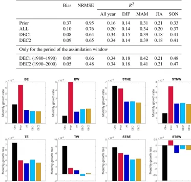
The observed FAPAR signal exhibits positive long trends, indicating a greening trend of vegetation for most of the re-gions, with the exception of the TSW region, where the long-term trend indicates a decrease in FAPAR (i.e., browning). In most of the regions, the assimilation results agree on a posi-tive long-term trend as in the observations; the magnitude of this trend is in disagreement with the observations (Fig. 3). Particularly in the BE region, the prior experiment overes-timates the FAPARobstrend by almost double. After the

as-similation, the simulated FAPAR trend is reduced, leading instead to a slight underestimation of the growth rate in all of the posterior experiments. In the TWS region, the assimila-tion improved the long-term trend from a positive to a nega-tive growth rate in the three posterior experiments. The most substantial disagreement between FAPARobsand FAPARmod

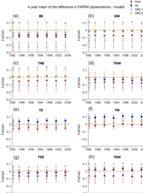
occurs in the TW region, where the observations show a pos-itive trend in FAPAR during the period of analysis, whereas this is not captured in the prior and all the posterior experi-ments. Despite these trend adjustments, the model–data error (based on the 4-year mean differences to the observations at regional scale) remains more or less constant across the 30-year period (Fig. 4).

The observed FAPAR signal also contains a small amount of interannual variability (Fig. S5). Compared to obser-vations, the simulated IAV of FAPAR (obtained from the monthly signal for each experiment) is improved only in the predominantly temperature-controlled boreal regions, whereas in temperate and tropical areas with a larger con-tribution of moisture-controlled phenology, the assimilation does not improve the variability (Fig. S5).

3.2 Atmospheric CO2

To diagnose the performance of the MPI-CCDAS with re-spect to the atmospheric mole fractions of CO2, we compare

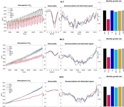
the observed and simulated values, in terms of the mean sea-sonal cycle, IAV, and monthly growth rate, at three stations: (1) Alert (ALT) in the Northern Hemisphere, (2) Mauna Loa (MLO) in the tropics, and (3) South Pole (SPO) in the South-ern Hemisphere. Results of this comparison are shown in Fig. 5. For MLO and ALT, the timing of the seasonal cy-cle is already well reproduced in the prior simulation, and the assimilation corrects errors in the amplitude of the sea-sonal cycle and the long-term trend. At SPO, there are also large relative differences between the model results and the observations, however, of a much smaller magnitude than for the two other stations. After the assimilation, the seasonal phase of CO2is shifted by approximately a month to better

Fig-Table 2.Statistical analysis of FAPAR for 1982–2006 in all of the experiments, and also for the periods of the window of assimilation only for DEC1 and DEC2.R2is obtained from the linear correlation between FAPARobsand FAPARmodcalculated for the entire period and by

seasons. NRMSE is the normalized root-mean-squared error, defined as RMSE divided by the mean (FAPARobs).

Bias NRMSE R2

All year DJF MAM JJA SON

Prior 0.37 0.95 0.16 0.14 0.31 0.21 0.33

ALL 0.10 0.76 0.20 0.14 0.34 0.20 0.37

DEC1 0.08 0.64 0.34 0.15 0.39 0.18 0.41

DEC2 0.09 0.65 0.34 0.14 0.39 0.18 0.41

Only for the period of the assimilation window

DEC1 (1980–1990) 0.09 0.66 0.34 0.18 0.42 0.21 0.48 DEC2 (1990–2000) 0.05 0.48 0.34 0.18 0.41 0.21 0.47

Figure 3.Mean monthly growth rate of FAPAR for 1982–2006 on each analyzed geographical region for the satellite observations and results of prior and the posterior experiments.

ure 6a shows a reduction in the CO2amplitude for stations

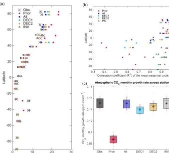
of the Northern Hemisphere (>40◦N) after the assimilation, which is in better agreement with the observations than the prior simulation. The most substantial amplitude reduction occurs at the northernmost station (ALT), where the seasonal amplitude decreases from 23.5 ppm in the prior experiment to 16.5 ppm in the ALL experiment, bringing it closer to the observed amplitude of 14.4 ppm. The latitudinal distribu-tion of the linear correladistribu-tion coefficient between the observed and simulated mean seasonal cycles is depicted in Fig. 6b, and demonstrates a very good agreement (R2>0.9) in the Northern Hemisphere in all of the experiments (including the prior simulation). In the tropics (specifically between 20 and 40◦N), the misfit of the phasing of the seasonal cycle is im-proved after the assimilation, as evidenced by an increased linear correlation. However, this is achieved at the expense of a considerable reduction in the amplitude of the seasonal

cycle compared to the observations. The results from the at-mospheric inversions (INV) show a closer statistical agree-ment with the observations, as shown in Figs. 5 and 6.

During the nearly 30 years of atmospheric CO2data

avail-able, the time series of the CO2mole fractions in the prior

model results strongly underestimate the long-term trend, and start to deviate in the first 5 years of the time series. In all the assimilation experiments, the long-term atmospheric CO2 trend is in much better agreement with the 30-year

Figure 4.Time series of the 4-year mean of the FAPAR anomaly for the satellite data for each model experiment in six selected model pixels. The error bar indicates the±1 standard deviation of the 4-year differences. The first marker (as asterisk) in the time series is the single value for 1982.

most notable deviations from the observed signals remaining unchanged after the assimilation procedure (Fig. 5).

3.3 Global and regional carbon pools and fluxes We next compare the simulated land carbon cycle in the prior and posterior experiments to independent data. In the posterior experiments, the vegetation C pool decreased be-tween 14 % and 20 % of the value in the prior but remained within the range of the literature estimate (442±146 PgC). The global soil C stock showed significant changes af-ter the assimilation. In all the posaf-terior experiments, the soil C pool decreased by 45 %, 43 %, and 53 % with re-spect to the value in the prior. Still, the total C in the soil (1362 PgC) in the ALL experiment after the assimilation is in closer agreement with the estimate from the Harmonized World Soil Database (http://webarchive.iiasa.ac.at/Research/ LUC/External-World-soil-database/HTML, last access: Jan-uary 2015) of 1343 PgC (Table 3). As for the total global vegetation C stock, the prior and assimilation are in closer

agreement with the lower end of the estimate by Carvalhais et al. (2014) (296 PgC).

The simulated latitudinal GPP values agree well with the data-driven model tree ensemble (MTE) estimate from Jung et al. (2011) for the period from 1982 to 2010 north of 30◦N. However, the assimilation results are low biased in the tropics, which propagated into lower estimates of global GPP in all the posterior results (Fig. 7d and Table 3). Af-ter the assimilation, the global GPP and NPP are reduced in the three posterior experiments compared to the prior (118.8 and 54.5 PgC yr−1, respectively). In contrast to the posterior global mean of GPP, the value in the prior simulation com-pares favorably well to the global mean from the MTE prod-uct (118.9 PgC yr−1) for the same period of analysis. The global mean GPP is reduced by up to 26 PgC yr−1 on aver-age in the three posterior experiments compared to the prior experiment. Simulation DEC1 experienced the largest reduc-tion in the global photosynthetic C uptake (83.1 PgC yr−1₎

relative to the prior value (Table 3 and spatial distribution of the GPP difference to the prior in Fig. S6d, f, and h).

At the large scale, the variation in the NBE (net biome exchange of CO2with the atmosphere, calculated as the net

ecosystem exchange (NEE) minus the flux related to land use change) from all of the simulations through the time series is similar to that from the Global Carbon Project 2017 (GCP17; Le Quéré et al., 2018) and INV, with the significant anoma-lies collocated in time (Figs. 7a, A4). Contrary to the prior simulation, the total annual NBE from the three posterior ex-periments falls within the uncertainty (shaded green area in Fig. A4d calculated as±1 standard deviation) of the mean NBE from the terrestrial ecosystem models in the GCP17. However, the 1982–2010 mean net biome exchange in all of the assimilation experiments through the time series is on average 1.4 PgC yr−1lower than the flux in the prior simula-tion (−2.06 PgC yr−1) and 0.8 PgC yr−1less than the GCP17 value (−1.27±0.97 PgC yr−1) (Table 3, Figs. A4d and S7 for summary of C balance).

In all MPI-CCDAS simulations, the NEE is reduced rela-tive to the prior in most of the Southern Hemisphere, while it is increased in the Northern Hemisphere (Fig. S6c, e, and g). Temperate northern areas contribute the most to the global net CO2 uptake. In the boreal east and west regions (BE

and BW), the net land C emissions increased in all of the posterior experiments compared to the prior (Fig. S6c, e, and g) with the most significant increase in BE for DEC2 (−0.29 PgC yr−1) relative to the corresponding value in the prior (−0.09 PgC yr−1_{). The decrease in GPP in the}

Figure 5.Statistical analysis of atmospheric CO2at three flask measurement sites: Alert (ALT; top panels), Mauna Loa (MLO, center panels),

and South Pole (SPO, bottom panels), from the measurements, prior, posterior experiments (ALL, DEC1, and DEC2), and inversion (INV1). For each station the panels show the time series of the mean monthly values, the mean seasonal cycle, the interannual variability, and the monthly growth rate for the entire period of the simulation (1980–2010).

The magnitude of the global NBE and GPP is smaller in the posterior experiments than in the prior. However, the trend in the anomaly of these fluxes (calculated relative to the temporal mean of each time series) is comparable in all the experiments (Fig. 7a and b), suggesting that the response to the environmental conditions is similar through the sim-ulation period after the assimilation as well. This robust re-sponse shows in GPP a similar and gradual increasing C up-take (positive trend) during the period of analysis, only with a slightly reduced slope in the prior experiment (Fig. 7b).

3.4 Prognostic capability of MPI-CCDAS

Finally, we evaluate the goodness of the model–data fit of the decadal assimilation runs with respect to their long-term carbon cycle simulation relative to (i) that of the prior and (ii) that of the assimilation run using data from the 30-year

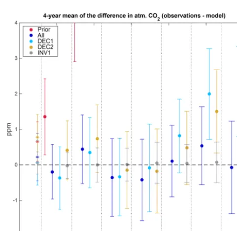
experiment as a reference case for “best possible” model– data match given the structural limitations of the MPI-CCDAS to match the observations (as evaluated in Sect. 3.1 and 3.2). We calculate the 4-year mean differences between the atmospheric CO2 mole fraction measurements and the

CO2model results and also the INV results, for all of the

sta-tions (Fig. 8). In the ALL assimilation experiment, the atmo-spheric CO2concentration consistently matches the

observa-tions across the entire assimilation period (that also corre-sponds to the window of assimilation) with a−0.03±1 ppm average bias to the observations (Fig. 8). This is comparable to the trend (Fig. 6c), and 4-year mean differences inferred by the inversions, where the 4-year mean results in the ALL fall within the standard deviation of the 4-year mean of the INV (Fig. 8). This is in striking contrast to the prior exper-iment, where the 4-year mean of the CO2mole fraction at

Figure 6. (a)Latitudinal distribution of the mean CO2seasonal amplitude for the 28 flask measurement stations from the observations, prior,

and posterior experiments.(b)Latitudinal distribution ofR2obtained from the correlation between the observations and each simulation result of the mean atm. CO2seasonal cycle and(c)average atmospheric CO2monthly growth rate across stations for the observations and

model results. The star on each bar is the mean of the atm. CO2monthly growth rate, the horizontal middle black line on each box is the

median, the red whiskers depict the error as 1 standard deviation, and the grey dots on each box are the actual monthly growth rate values for all the stations in each data set.

Table 3.Global average of the terrestrial carbon cycle components and carbon stocks in results from the assimilation experiments and prior (1982–2010), and other independent estimates (see table footnote for description).

Prior ALL DEC1 DEC2 INV Literature

GPP (PgC yr−1) 118.8 96.9 83.1 97.2 – 118.9a

NPP (PgC yr−1) 54.5 34.2 37.3 30.3 – –

NEE (PgC yr−1) −2.64 −1.13 −1.32 −1.18 −1.20c −2.52±0.98b NBE (NEE+LULCC) (PgC yr−1) −2.06 −0.54 −0.74 −0.60 – −1.27±0.97b

ER (PgC yr−1) 115.7 95.2 81.0 95.3 – –

Ra (PgC yr−1) 64.2 62.7 45.8 66.9 – –

Rh (PgC yr−1) 51.5 32.4 35.2 28.4 – –

Root exudates (PgC yr−1) 3.3 2.0 2.2 1.7 – –

Soil C (PgC) 2481 1364 1423 1167 – 1343d

Vegetation C (PgC) 394 310 335 311 – 442±146e

Litter C (PgC) 228 166 171 158 – –

a_{Model tree ensemble data-driven product; Jung et al., 2011; average for 1982–2010.}b_{Global Carbon Project (2017), Le Quéré et}

al. (2018); average for 1982–2010. The NBE values include the LULCC reported for each individual model.cInversion result is the average for 1982–2009.dhttp://webarchive.iiasa.ac.at/Research/LUC/External-World-soil-database/HTML (last access: June 2015).

Figure 7.Time series of the anomaly to the temporal mean of the time series(a, b), and latitudinal gradient(c, d)of the total net ecosystem exchange (NEE including the influence of LULCC)(a, c)and gross primary production(b, d)for the results of each model simulation. NEE from the model is compared to the GCP 2017 and INV data set(a, c). GPP is compared to the MTE data-data driven estimate of Jung et al. (2011)(b, d).

For the DEC1 experiment, the 4-year mean difference among the measurements and the model results is between−0.3 and 0.3 ppm in the 1980s. This level of model–data agreement re-mains for the 1990s, where the experiment did not see any observations. After the year 2000, the fit increasingly de-grades, with an underestimation of the CO2 mole fraction

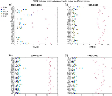
by 1.6 ppm for the last 4-year average. However, this is still a 90 % reduction in misfit compared to the prior experiment. We next quantify the RMSE between the CO2

measure-ments and model results for each station for four differ-ent periods: 1982–1990, 1990–2000, 2000–2010, and 1982– 2010 (Figs. 9 and A2). The large bias of the prior is re-flected in the RMSE where the results of this experiment have the most substantial error for all of the stations and periods (between 2.8 and 18.7 ppm) (Fig. 9). For the pos-terior experiments with a decadal window of assimilation (DEC1 and DEC2), the performance of the assimilation of CO2mole fraction also improves substantially across all time

periods. Within the period of the assimilation, the difference to the measurements and RMSE is most strongly reduced, and the error increases somewhat outside of the window of assimilation. The model results show that when only the first decade of data is assimilated (DEC1), a more significant de-viation to the long-term trend of atmospheric CO2occurs

be-tween 2000 and 2010 compared to DEC2 and ALL (Fig. 9c). Similarly, a larger bias is also observed in the results from DEC2 where the lowest 4-year mean difference between the observations and the assimilation results takes place in the period of the window of assimilation for this experiment (1990–2000) (Figs. 8 and 9b for RMSE). During this period, the model overestimates the CO2atmospheric concentration

only by 0.15 ppm on average, whereas for the periods

out-Figure 8.Time series of the 4-year mean of the atm. CO2anomaly

Figure 9.RMSE for different periods between CO2atm. concentrations from measurements and model results for the different assimilation

experiments and inversion results for each of the flask measurement stations.

side the window of assimilation, the CO2 concentration is

underestimated by 0.64 ppm in the period 1982–1990, and by 1.04 ppm in the period 2000–2010. Thus, in experiment DEC2 the prognostic skill of CCDAS is also reduced outside the window of assimilation, and the long-term trend is less well reproduced than in the ALL experiment.

The analysis of the 4-year mean differences for the pe-riod 1982–2006 between FAPARobs and the results of the

prior and assimilation experiments at the regional scale (ar-eas in Fig. 1) reveals, contrary to the CO2 observations,

a near-constant 4-year mean FAPAR difference within the time series and each of the experiments (Fig. 4). In general terms, the decadal experiments are better able to reproduce the mean FAPAR across all regions. The largest difference between posterior results to the observations is in the tropical regions, where the FAPAR 4-year mean difference showed that the observations remained consistently larger than the ALL results by on average 0.042 in TE and 0.095 in TW (Fig. 4). Importantly, however, the trend correction for the

boreal and temperate areas (Fig. 3) is similar across the dif-ferent assimilation experiments, suggesting that important biases of the JSBACH 3.0 model, including the tendency to simulate too strong boreal greening, can be readily reduced with only 10 years of data, as further improvement with the 30-year record is small.

4 Discussion

The parameter optimization with a simultaneous assimila-tion of long-term spaceborne FAPAR and atmospheric CO2

measurements in the MPI-CCDAS, resulted in a consider-able reduction in the cost function and norm of the gradient, which can be seen as an overall improvement in the mod-eled global carbon fluxes with a decrease in the root-mean-squared error of the MPI-CCDAS compared to the CO2and

parame-ters were consistently retrieved after the assimilation, such as the maximum leaf area of grasses and shrubs and the correc-tion parameter for the initial soil pool size, some final param-eter estimates varied considerably between the three experi-ments, e.g., the tropical maximum leaf area index and some of the parameters controlling the seasonality of the phenol-ogy (Fig. A3). These variations lead to regional differences in the simulated compartment flux GPP and ecosystem respi-ration, which are not well constrained from the observations. Interestingly, these differences result in very similar absolute values in global carbon fluxes and their trends. This demon-strates a certain degree of equifinality in the results and cau-tions a too stringent interpretation of the MPI-CCDAS out-come in terms of improving understanding about biosphere processes and their long-term trends.

4.1 FAPAR

MPI-CCDAS is capable of extracting information about the seasonal cycle and the long-term trends from the FAPAR ob-servations. Using decade-long FAPAR data during the assim-ilation (DEC1 and DEC2) already leads to notable improve-ment of the simulated seasonal phenology of the land surface within and outside the window of assimilation, i.e., main-taining these changes during the prognosis periods. This im-provement is predominantly the result of the ability in the model to simulate the timing of green-up and brown-down in spring and summer through the optimization of parame-ters that regulate the onset and end of the growing season (i.e., parameters for temperature and day-length thresholds). The greening effect is especially taking place in the Northern Hemisphere, dominated by the phenotypes deciduous and ev-ergreen needleleaf and extratropical deciduous trees.

The long-term greening trend in the vegetation of boreal regions previously observed in spaceborne data (Forkel et al., 2016; Lucht et al., 2002) was captured in the results of MPI-CCDAS before the assimilation, but it was mostly overestimated in northern regions and underestimated in the Southern Hemisphere. After the assimilation experiments, the greening trend was improved primarily in the boreal areas and is in closer agreement to the reported satellite FAPAR data. The modest improvements achieved in the simulated greening trend of temperate areas in the western hemisphere are associated with a decreased performance in the east-ern hemisphere, indicating that the model structure of MPI-CCDAS is incapable of reconciling regional differences. This difference could be an indicator of the need to parameterize both hemispheres differently in terms of their phenological response to the underlying driving factors (such as temper-ature, moisture availability, and day length); also, this could be due to the lack of process to account for the land use or vegetation dynamics in the MPI-CCDAS.

Despite these broadscale improvements, the MPI-CCDAS does not reproduce the magnitude of the greening trend and its interannual variability in all the posterior experiments at pixel and regional levels. This is likely a result of the MPI-CCDAS structure, which relies on few globally relevant PFT-level parameters. Although some of the phenological param-eters in CCDAS adapt to local mean growing season temper-ature, other thresholds are only globally applicable, causing a trend to temperature grasslands that cover a wide climato-logical range. For example, some of the global parameters such asfaut_leafandfslow imply that improvements of

mod-eled fluxes in the boreal regions directly affect fluxes in the tropics, inducing parameter changes to compensate for the altered C fluxes. Defining instead such global parameters per PFT would alleviate this issue but will compromise the com-putational cost and might not necessarily reduce the over-all uncertainty. Another technical chover-allenge is the use of a spatially mixed signal at the coarse spatial model resolution (due to the high computational requirements necessary to in-crease model resolution) to infer PFT-specific parameters. A likely better strategy for constraining PFT-specific parame-ters would be to resample the highly resolved satellite prod-uct to PFT-specific FAPAR classes per pixel before the ag-gregation into a global grid. This change would allow us to find more spatially refined classes and provide PFT-specific FAPAR maps to the CCDAS to reduce issues in the identi-fication of phenological parameters for different climatic re-gions.

Except for the tropical latitudes, the difference between the regional IAV of the observations and model output is small compared to seasonal variations. The modeled signal remains within a range of 0.05 (dimensionless) FAPARobs. The

sig-nal and the model–data difference is also smaller than the global mean retrieval error of the FAPAR product, which is ±0.2088 (Schürmann et al., 2016). This error was used to quantify the observational FAPAR uncertainty in the assim-ilation, thereby reducing the ability of the MPI-CCDAS to detect and correct such smaller variation. Overall, the lack-ing match of the IAV may therefore be of little overall con-cern. Nevertheless, the lower than observed IAV in the trop-ical bands may be indicative of too weak drought response in the maximum leaf area index of the model. Although the assimilation procedure allows changes in the phenology re-sponse to water stress (given by parameterτw), the

assimi-lation procedure decreased the drought sensitivity of tropi-cal phenology given the entire spatially explicit FAPAR time series, and therefore did not allow capture of the regional drought events that could be in principle linked to changes in LAI.

The technical error during the assimilation procedure to not include the period from 2007 to 2010 in the FAPARmod

with little effect on the overall trends between the three as-similation experiments with different time periods.

Bearing in mind the different spatial resolution of meth-ods (i.e., model grids and remote-sensing pixels), a robust comparison between the mean and maximum LAI values be-fore and after the assimilation per region are presented in Table A1 of the Appendix. The results fall within LAI values from MODIS and lidar reported in the literature. Ground-based observations in the tropical Amazon–savanna transi-tion forest between 2005 and 2008 show an annual mean LAI value for the total canopy of 7.4±0.6 m2m−2, and for the seasonally flooded forest the value of 3.4±0.1 m2m−2. For the remote-sensing data from MODIS, the reported values are 6.2±0.2 and 5.8±0.3 m2m−2, respectively (Biudes et al., 2014). In the eastern Amazon forest, the remote-sensing-based LAI has been reported as 6.2 m2m−2from lidar, and 4.8 m2m−2_{with a low end of 2.0 m}2_m−2_{from MODIS (Qu}

et al., 2011).

4.2 Atmospheric CO2

The considerable improvement of the seasonal amplitude and the long-term trend of atmospheric CO2 at Northern

Hemi-sphere stations is independent of the different periods of data used for the assimilation. However, the MPI-CCDAS consis-tently fails to resolve some of the features of the year-to-year variability detected in the measured atmospheric CO2

sta-tions, which translates into an acceptable, but far from per-fect fit to the inferred annual carbon budget of the GCP17 (Le Quéré et al., 2018). We compared the performance to the results from an atmospheric CO2 inversion (INV) with the

same input fields and atmospheric transport model as MPI-CCDAS to illustrate that these deviations do not reflect un-certainties in the representation of the atmospheric transport. It needs to be mentioned that both the choice of the atmo-spheric transport model (and associated imperfections at re-solving the vertical and lateral atmospheric transport of CO2)

and the method to aggregate atmospheric observations to ob-tain an estimate of the annual growth rate in the global car-bon budget introduce some error in any forecast of the inter-annual variability. As a consequence, only the occurrence of more significant model–data mismatches can be interpreted as an actual result of the MPI-CCDAS’ inability to correctly resolve the carbon flux variation.

Notably, the model lacks the representation of some key processes that contribute to climate-induced interannual vari-ability of the carbon cycle, such as the possibility to dynami-cally account for fire disturbance (Lasslop et al., 2014), trop-ical peatland fires related to El Niño–Southern Oscillation (ENSO) (van der Werf et al., 2008), or the increase in terres-trial carbon uptake after large-scale volcanic eruptions such as for Mt. Pinatubo in 1991 (Lucht et al., 2002; Mercado et al., 2009). Omitting fluxes in the current model configuration due to fire events may impair the ability of the model to in-fer the atmospheric growth rate of CO2 associated with El

Niño events (Frölicher et al., 2011, 2013). One way to over-come the IAV mismatch would be to include fire fluxes in the model by prescribing them from the Global Fire Emis-sions Database (GFED; van der Werf et al., 2010); however the latest version of this data set (version 4.0) is only avail-able for years from 1997, which is a limiting factor for the timeframe of the simulations in this work. However, the con-tribution of these interannual variations to the overall CO2

cost function is low in comparison to the signal contained in the seasonal cycle and deviations in the long-term trend, such that the MPI-CCDAS may simply not be sensitive enough to these aggregate system properties like the response of the tropical carbon cycle to El Niño events given the uncertainty in the atmospheric transport and the observational represen-tation error.

4.3 Carbon cycle simulation

Independent of the amount of data used in the assimilation window, our results show that the GPP and NEE were con-sistently reduced globally compared to the prior run, i.e., less carbon uptake by plants leading to the model results being in closer agreement with other independent estimates such as the GCP17. The MPI-CCDAS suggests a somewhat lower average annual atmospheric CO2 growth rate

(calcu-lated by the sum of the net C fluxes from the ocean, land, and fossil fuel emissions) than the one estimated in the GCP17 (Le Quéré et al., 2018), even if the MPI-CCDAS estimate falls within the uncertainty of the GCP17 (Figs. 7 and S7). Most of the difference stems from small differences in the assumed fossil and ocean carbon fluxes. In the case of the carbon fluxes from fossil fuels, the data prescribed in MPI-CCDAS do not contain fluxes due to cement and flaring; thus the magnitude of the annual carbon sources through the time series is consistently lower but still within the±5 % uncer-tainty of the GCP17 data (Le Quéré et al., 2018) (Fig. A4). As for the ocean carbon sink, the annual mean values pre-scribed in MPI-CCDAS are also of lower magnitude than the mean value in the GCP17 but falling in the lower limit of the uncertainty value (Figs. A4c and S7). The flux due to LULCC prescribed in MPI-CCDAS is also of smaller magni-tude than that from the GCP17 because the simulation made by JSBACH 3.0 does not consider disturbances like fires and gross transitions, which might have also contributed to the lower land C sink obtained in the assimilation experiments compared to the total land C sink in GCP17 (Fig. A4d).

fea-ture is likely the result of a global compensating effect on heterotrophic respiration, and this effect is observed in the drop of the photosynthetic capacity (fphotos) in the tropical

evergreen and deciduous PFTs, as well as in the reduction of the maximum tropical LAI in the three assimilation ex-periments compared to the prior. In addition, another critical factor influencing the global reduction of GPP and the trop-ical uptake of C appears to be related to the difference in data availability of CO2stations between the defined

assim-ilation windows. Specifically, this is evident in the results of the data-poorer experiment DEC1, where the topical GPP is substantially lower than in the independent estimates and in the assimilation experiments that use more stations (DEC2 and ALL). As a result, the mean tropical land C source to the atmosphere in the prior experiment (mean NBE value of 0.12 PgC yr−1, and minimum value of −0.07 PgC yr−1, re-flecting C uptake in the 4◦_{S latitudinal band) was increased}

to 0.37±0.17 PgC yr−1_{on average for all the posterior}

re-sults.

The NPP:GPP ratio in ALL and DEC2 decreased to 0.35 and 0.31, respectively, when compared to the prior value (0.45). This reduction might be mainly because the NPP is not well constrained from the atmospheric record. In JS-BACH 3.0, autotrophic respiration (Ra) is directly coupled to GPP; hence the fraction of GPP partitioned to Ra leads to an increase in the seasonal cycle of the ecosystem respiration. An increase in Ra with respect to the prior (which is only vis-ible in the global average value in DEC2; Table 3) results in a reduced net land carbon uptake, masking the smaller changes in the vegetation turnover.

The reduction in the soil C pool after the assimilation can be explained due to an unavoidable effect in the model. The MPI-CCDAS was initially spun up until the soil C pools reached equilibrium considering preindustrial forcing; how-ever, this new initial state does not consider climate variabil-ity. To compensate for this and to reduce the respiration when the MPI-CCDAS is confronted with contemporary changes in the climate, the model creates an artificial C sink that leads to a reduction in the soil C stocks. It is important to note that the JSBACH 3.0 version used in this MPI-CCDAS does not include permafrost processes; therefore, the global soil C stock might still be underestimated.

4.4 Value of long-term data sets to constrain CCDAS Notwithstanding the MPI-CCDAS conceptual issues, the setup of this study enables us to test by how much the quality of the data–model agreement is reduced after exposing the MPI-CCDAS to shorter observational time series. In terms of FAPAR, there is no apparent degradation of fit with time, despite that in general terms, the trend in the data is best matched with the ALL experiment. This is foremost a con-sequence of comparatively small trends in the observed FA-PAR, implying that extracting the mean seasonal patterns and amplitude for a few years is essential for simulating current

and near-term FAPAR. Issues with model structure and with the assimilation setup prevent a better model–data fit irre-spective of the length of the record. This would suggest that a focus of assimilation on high-quality and highly spatially re-solved FAPAR should be a priority over the use of long-term data sets. The results are different for the case of projecting atmospheric CO2, where a long record of atmospheric CO2

measurements favorably contributes to a better representa-tion of the long-term values after the assimilarepresenta-tion, whereas a shorter window leads to deviations to the observations in the periods outside the assimilation years. The model–data agreement is of approximately±0.5 ppm during the assimi-lation period and starts to deviate for the DEC1 experiment later than 10 years after the end of the assimilation win-dow, whereas in the DEC2 experiment, the degradation of the model–data match already starts after approximately 5 years. Still, the average deviation from the observations by using shorter assimilation periods is not far from the upper limit of the uncertainty when using the longest record. Nonetheless, with the caveat that MPI-CCDAS does not fully explain the interannual variability of the land net carbon flux, this sug-gests a reasonable short-term (for a small number of years) forecasting skill of atmospheric CO2.

5 Conclusion

The MPI-CCDAS is capable of simultaneously integrating two independent observational data sets over three consec-utive decades at the global scale to estimate global car-bon fluxes. The results demonstrate that assimilating only 1 decade of observations, for two observational data sets (FA-PAR and atmospheric CO2concentrations), leads to broadly

comparable results and trends in the global carbon cycle components than using the entire time series of available ob-servations (30 years). Currently, the system can confidently predict the carbon fluxes on short timescales (up to 5 years after the end of the window of assimilation), e.g., for atmo-spheric CO2 concentrations at the site level, and the mean

prediction remains within the uncertainty of the observations. However, long-term forecasts with CCDAS are less certain, as the observational record does not sufficiently constrain the interannual variability of the simulated land carbon fluxes and longer-term changes in the decadal net carbon uptake. Nevertheless, the comparatively small error of 2±1.3 ppm after 15–19 years of prognostic simulation shows the poten-tial for midterm carbon cycle predictions constrained using the CCDAS approach.

the land C uptake, suggesting that further improvements in the land surface model, especially in the current structure and design, must be first solved to improve the model and com-putational efficiencies of the system. This is recommended before an attempt to include another observational stream or other modifications aiming to test an enhancement on the prognostic skill in the full MPI-CCDAS.

Code availability. The code of the JSBACH model is available

Appendix A

A1 Assimilation performance

Figure A3 depicts the final posterior value (Xf) for each

op-timization parameterI and in each assimilation experiment. The last parameter value is normalized to its corresponding prior value (Xp, shown in Table 1), i.e., (Xf/Xp)−1; this is

done to make a comparison between parameters on their re-sponse and the assimilation because each parameter holds a different range of values. The normalized result is also shown for each phenotype for the phenology and photosynthesis-related parameters, and also for the initial leaf growth rate (ξ), CO2initial offset, and land carbon turnover parameters

that are applied globally.

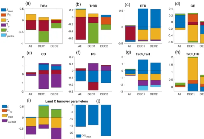
More significant changes in some phenology parameter values are observed; e.g., the maximum LAI (3max)

de-creased in almost all PFTs and in all experiments, except for the phenotypes CE (coniferous evergreen) in the ALL exper-iment and ETD (temperate broadleaf evergreen and decidu-ous; mostly dominating in Europe and the eastern USA and Asia). In CD (coniferous–deciduous trees; located in north-east Asia, specifically in the north-east Siberian taiga) the 3max

value increased notably in the DEC1 and DEC2 experiments (Fig. A3e).

In the tropical forest areas, the reduction of the3maxwas

from 3.17 in the prior experiment to 2.27 (33 %) in ALL for the TW area, and from 3.27 in the prior to 2.43 (26 %) in ALL for the TE area. For the other assimilation experiments the average maximum LAI moderately decreased in TW from 3.17 in the prior to 2.89 (8.8 %) in DEC1 and from 3.17 in the prior to 3.00 (5.3 %) in DEC2.

In other extratropical areas results from experiments DEC1 and DEC2 experienced an average increase in 3max

by 5.6 % in BE (from 2.29 in the prior to 2.42), 24 % in BW (from 1.62 in the prior to 2.01), and 3.8 % in TNW (from 3.11 in the prior to 3.23).

As a result, the temperature- and daylight-related param-eters were modulated such that the largest decrease with re-spect to the prior value in the temperature at leaf onset (T ϕ) was also observed for these two PFTs, especially for CD in the DEC1 and DEC2 experiments. Also, the day length at leaf shedding (tc) and the timescale of leaf senescence (leaf shedding timescale, 1/τ1) primarily increased for CD.

As for the PFTs influenced by temperature and water (TeH, TeCr, TrH, and TrCr), the most significant change with re-spect to the prior value took place in the posterior value for the C3crops (TeCr; distributed in Europe, the USA, and

East Asia) whose value decreased considerably for the wa-ter stress tolerance (τw) in experiments DEC1 and DEC2,

whereas the value of the timescale of leaf senescence (leaf shedding timescale, 1/τ1) also increased considerably for the

same experiments. These changes seemed to be a response of the large decrease in the foliar area3maxfor this PFT, which

took place in all three experiments. The value of the

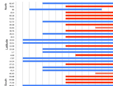
photo-Figure A1.Data availability and latitudinal location of the 28 sta-tions where the long-term flask measurements of atmospheric CO₂ mole fractions were taken for assimilation in CCDAS. The ALL experiment used all the stations of the time series (blue and red bars) (1980–2010), DEC1 used data only from stations with blue bars (1980–1990), and DEC2 also used the data at the stations with red bars (1990–2000) (except stations SBL and CRZ marked with a patterned bar).

Figure A2. Experimental setup for posterior experiments ALL, DEC1, and DEC2 with different temporal windows for the assimi-lation of FAPAR and molar fractions of atmospheric CO2.

synthesis rate modifier (fphotos) influences the productivity

at leaf level. Thus, a lower value offphotoswill lead to lower

GPP (less carbon uptake and a potential increase in NEE). Our results show that after the assimilation experiments the value offphotos decreased with respect to the prior

experi-ment, mainly for the C3grasses and pasture (TeH; distributed

mostly in the Northern Hemisphere) as well as for the tropi-cal evergreen and deciduous trees (TrBE and TrBD), and this is more noticeable in the DEC1 experiment.

As for the global parameters, significant deviations from the prior value are observed in the parameter that controls the initial size of the slow soil C pool (fslow) and also in the

parameter that defines the initial atmospheric CO2mole

Figure A3.Final value for each parameterpat the end of the assimilation experiments, normalized to the prior value (ppr), i.e.,(p/ppr)−1. This is shown for each model plant functional type(a–h)and globally for the land C turnover parameters(i, j).

Table A1.Regional mean and maximum leaf area index in prior and posterior experiments.

Region Prior ALL DEC1 DEC2

(LAI (LAI (LAI (LAI

mean; max) mean; max) mean; max) mean; max) (m2m−2) (m2m−2) (m2m−2) (m2m−2)

BE 0.61; 2.29 0.60; 1.94 0.70; 2.42 0.69; 2.42 BW 0.31; 1.62 0.30; 1.44 0.35; 2.01 0.35; 2.02 TNE 1.28; 4.28 1.17; 3.33 1.31; 3.49 1.32; 3.79 TNW 1.26; 3.11 1.15; 2.84 1.30; 3.23 1.30; 3.21 TE 1.62; 3.27 1.30; 2.43 1.63; 3.20 1.67; 3.33 TW 2.21; 3.17 1.68; 2.27 2.00; 2.89 2.08; 3.00 TSE 1.54; 2.72 1.43; 2.51 1.86; 2.77 1.83; 2.68 TSW 2.42; 3.69 2.04; 2.71 2.38; 3.47 2.43; 3.66

the global heterotrophic respiration, controlling in this way the disequilibrium between GPP and the ecosystem respira-tion. Because JSBACH tends to overestimate the soil C pool, optimizingfslowis a means to improve this estimation;

how-ever, the spatial distribution of the carbon pools remains un-changed, and the prior value controls the prior value, mean-ing that the GPP and ER relation remains similar in the pos-terior experiments to that in the prior experiment. Since the magnitude of the initial slow carbon pool was set, this might influence the other modeled carbon pools compared to the soil carbon pool, leading to biased soil and vegetation car-bon stocks; therefore, the assessment on the predicted pools should be made with care. We compare the resulting global total soil and vegetation carbon pools robustly to independent

estimates from the literature or other products, and results are shown in the main text of the Discussion section.

A2 Pixel-level phenology analysis

The FAPAR analysis at the pixel level shows that in pixels P1 (located in eastern Siberia), P2 (located in eastern Brazil), and P6 (located in Canada), the magnitude of the mean sea-sonal cycle is better represented when compared to the obser-vations (Fig. S4). Also, the timing of the mean seasonal cycle is corrected, e.g., in pixels with large seasonal amplitude such as in P1 and in P6. While in the prior experiment (and ALL experiment) the onset and peak of the growing season in P1 and P6 are delayed by up to 2 months, in the results from experiments DEC1 and DEC2 this delay is reduced to only 1 month. This correction might be partially due to changes in some optimized parameters: increase in the day length at leaf shedding (tc) and reduction in the temperature at leaf onsetT ϕ detected for both the CE and CD, as well as for ETD, TeCr, and TeH phenotypes (Fig. A3c, d, e, and g); this is because these parameters control the onset and end of the vegetation activity. Despite changes inT ϕandtcafter the as-similation in TrH, this temporal shift is less evident in P2. In this pixel, the amplitude of the seasonal cycle is small, and only changes in the magnitude of the amplitude are visible after the assimilation (Fig. S4). In the results of DEC1 and DEC2 for pixel P3 (located in the USA and dominated by TeCr), the water stress tolerance time (τw) andT ϕwere

pri-marily reduced, whereas the leaf shedding timescale (1/τl;

Figure A4.Time series of the annual mean of the major components of the C cycle used as background fluxes in CCDAS compared to those from the GCP 2017. The atm. CO2growth from the model output is the result of the sum of fossil fuel, ocean, and land C fluxes. The blue