Construction of Multi-Mode Fiber Modes using Phase Masks

Rochester Institute of Technology

RIT Scholar Works

Theses Thesis/Dissertation Collections

8-9-2013

Construction of Multi-Mode Fiber Modes using

Phase Masks

Alexandre Tulikumwenayo

Follow this and additional works at:http://scholarworks.rit.edu/theses

Part of theSystems and Communications Commons

This Thesis is brought to you for free and open access by the Thesis/Dissertation Collections at RIT Scholar Works. It has been accepted for inclusion

Recommended Citation

Rochester Institute of Technology

College of Applied Science and Technology

Electrical Computer and Telecommunications Engineering Technology

(ECTET)

Construction of Multi-Mode Fiber Modes

using Phase Masks

Alexandre Tulikumwenayo

August 09, 2013

Rochester, New York, USA

A Research Thesis Submitted in Partial Fulfillment of the Requirements

for the degree of

Masters of Science in Telecommunications Engineering Technology

Thesis Supervisor

Professor Dr. Drew N. Maywar

Department of Electrical Computer and Telecommunications Technology

College of Applied Science and Technology

Rochester Institute of Technology

Rochester, New York

Approved by:

Dr. Drew N. Maywar

Thesis Advisor, Department of Electrical Computer and Telecommunications

Engineering Technology.

Prof. Mark J. Indelicato

Committe Member, Department of Electrical Computer and

Telecommuni-cations Engineering Technology.

Dr. Sungyoung Kim

Committe Member, Department of Electrical Computer and

Abstract

Transverse fiber modes are the distribution of electromagnetic fields in the

cross-section of an optical fiber through which light propagates in the fiber.

Research is being conducted to explore the usage of fiber modes with the

purpose of increasing the capacity and reach of optical fibers. Mode Division

Multiplexing, an area in which reseach is being conducted with the same

purpose, is a multiplexing scheme used in optical networks that maps data

channels onto different modes, and multiplexes these modes into one fiber for

transmission. This thesis focuses on the study of modes in multi-mode fibers,

and the simulation of mode creation in gradient-index multi-mode fibers.

Starting from published related works, equations for electric fields in

step-index and gradient-step-index multi-mode fibers are derived, and examples of

intensity profiles in several modes are shown. For the first time, we seek

to study modal cross-talk between modes. Given the creation process, not

all power is coupled into the desired mode, resulting in some power being

coupled into undesired modes. We also seek to increase the power coupling

between the created mode and the desired mode. We report a 23% power

coupling increase up from previous works. Finally, we seek to study the effect

of noise introduced by the components used in the process of creating modes.

We report an approximate 30dB signal-to-noise ratio is sufficient to create a

Contents

1 Introduction 1

1.1 Telecommunications Optical Fibers . . . 2

1.2 Modal Dispersion . . . 3

1.3 Mode Division Multiplexing . . . 4

1.4 Thesis Overview . . . 5

1.4.1 Previous Related Work . . . 5

1.4.2 Advancement of the State of the Art by the Current Thesis . . . 6

2 Mode Theory in Multi-mode Fibers 8 2.1 Geometry of Fibers . . . 8

2.2 Multi-mode Step-index Fibers . . . 10

2.2.1 Electric Field in Multi-mode Step-index Fiber . . . 10

2.2.2 Eigenvalues of Multi-mode Step-index Fibers . . . 14

2.2.3 Intensity Profiles of some Step-index Modes . . . 18

2.3.1 Electric Field in Multi-mode Gradient-index Fibers . . 22

2.3.2 Orthogonality of Gradient-index Fiber Modes . . . 23

2.3.3 Intensity Profiles of some Gradient-index Modes . . . . 26

3 Transverse-Mode Phase Masks 28 3.1 Construction of Fiber Modes using a Spatial Light Modulator 32 3.2 Unit Amplitude . . . 35

3.2.1 Results . . . 35

3.3 Optimal Aperture . . . 38

3.3.1 Abbe’s Theory . . . 38

3.3.2 Aperture Diameter Optimization . . . 40

3.3.3 Results . . . 46

3.4 Optimal Inner Aperture Block . . . 49

3.4.1 Results . . . 53

4 Far-field Phase Noise 56 4.1 SLM Noise . . . 56

4.2 Effect of SLM noise on creation of modes . . . 57

5 Concluding Remarks 60

Appendices 65

List of Figures

1.1 Inter-symbol Interference due to Modal Dispersion in

Multi-mode Fibers. . . 3

1.2 Four data channels are mapped to four different modes in a

Mode Division Multiplexing system. . . 5

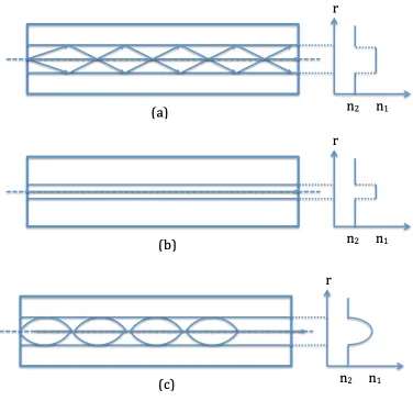
2.1 Refractive index profile in: (a) multi-mode step-index fiber,

(b) a single-mode step-index fiber, and (c) a multi-mode

gradient-index fiber. . . 9

2.2 Graphical solution for multi-mode step-index E0,m and E1,m.

modes . . . 16

2.3 Graphical solution for multi-mode step-index E3,m and E4,m.

modes . . . 17

2.4 Intensity plots for four E modes in multi-mode step-index fiber. 19

2.5 Power-law refractive-index profile n(r). . . 20

2.6 Intensity plots fo four modes in gradient-index fiber. . . 27

3.2 In the far-field (a) Image A amplitude, (b) Image A phase, (c)

Image B amplitude a, (d) Image B phase. . . 30

3.3 Reconstructed Images (a) Amplitude of Image A with phase of Image B, (b) Amplitude of Image B with phase of Image A. 31 3.4 Construction of Fiber Modes using a Spatial Light Modulator. 32 3.5 Power Coupling and Modal Cross-talk for mode E0,1. . . 36

3.6 Power Coupling and Modal Cross-talk for mode E3,2. . . 37

3.7 Abbe’s Theory of Imaging. . . 39

3.8 Frequency Component of Mode E04. . . 41

3.9 An aperture is placed in front of SLM to block high frequencies. 42 3.10 Change ofη with respect to the highest allowed frequency for angular-independent modes (El=0,m). . . 44

3.11 Change ofη with respect to the highest allowed frequency for angular-independent modes (El6=0,m). . . 45

3.12 Power Coupling and Modal Cross-talk for Mode E0,1: Com-parison between Unit Amplitude and Optimal Aperture Setups. 47 3.13 Power Coupling and Modal Cross-talk for Mode E3,2: Com-parison between Unit Amplitude and Optimal Aperture Setups. 48 3.14 Lower frequencies do not exist in the spectrum of angular-dependent modes. . . 50

3.16 Change of η with respect to the lowest allowed frequency for

angular-dependent and angular-independent modes. . . 52

3.17 Percentage Increase in Power Coupling: Increasing Azimuthal

Mode Number. . . 54

3.18 Percentage Increase in Power Coupling: Increasing Radial Mode

Number. . . 55

4.1 Effect of SLM noise of mode creation. . . 58

4.2 Impact of SNR on Power Coupling. . . 59

A.1 Graphical solution to eigenvalue equation. The solution is the

Chapter 1

Introduction

The ever growing demand for higher speeds of information transmission is

leading to the exploration of new and more efficient ways of transmitting

information. As the existing high speed links are approaching their full

ca-pacity [1], it is imperative to explore new ways to accommodate the demand

for high speeds, and to provision for future higher speeds demand. This

demand is more accentuated in data centers and other local-area networks

(LAN), as the amount of information to transmit in these networks keeps

increasing. Multimode fibers (MMF) are the type of fibers widely employed

in these networks [2]. It is desired to transmit data at 10 Gb/s and higher bit

rates over long distances of MMF, but the modal dispersion in these fibers

1.1

Telecommunications Optical Fibers

There are mainly three types of optical fibers utilized in the

Telecommunica-tions industry: single-mode fiber, step-index multi-mode fiber, and

gradient-index multi-mode fiber. Single-mode fibers have a smaller core of a high

refractive index n1 surrounded by a cladding of a low refractive index n2.

Because of the small size of the core, single-mode fibers allow only one

dis-tribution of electromagnetic field, namely mode. They are generally used in

long haul communications. Step-index and gradient-index multi-mode fibers

are types of multi-mode fibers. Multi-mode fibers have a larger core

com-pared with single-mode fibers. In step-index multi-mode fibers, the refractive

index of the core is constant across the core and is higher than that of the

cladding. Gradient-index multi-mode fibers have a varying refractive index

in the core, following a decreasing power law with the maximum value at the

1.2

Modal Dispersion

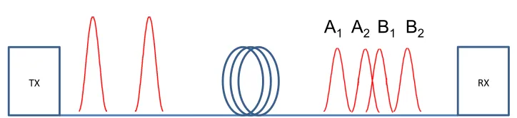
TX   RX  

A B

A₁ A₂ B₁ B₂

Figure 1.1: Inter-symbol Interference due to Modal Dispersion in Multimode

Fibers.

As light, encoded with information to transmit, is launched in a MMF,

sev-eral different transverse modes are excited in which light propagates [3]. The

existence of these modes depends on the launch condition at the transmitter,

among other dependencies. The choice of MMF in LAN is based on the ease

of light launch into the fiber, and therefore a less expensive infrastructure

over single mode fibers (SMF). Since these modes have distinct group

ve-locities, the information carried by the modes reach the receiver at different

times. This physical phenomenon is known as modal dispersion. The direct

effect of modal dispersion is Inter-symbol Interference (ISI). A pulse leaving

the transmitter reaches the receiver after having overlapped with its

neigh-boring pulse [3]. Figure 1.1 shows two distinct pulses at the transmitter and

the subsequent four pulses at the receiver. ISI due to modal dispersion in

communications systems [3].

There have been numerous approaches to compensate for modal

dis-persion effects using digital signal processing [14] and other inline techniques

using adaptive optics. The compensation for modal dispersion using a spatial

light modulator (SLM) proves to be more efficient since it does not require

a prior knowledge of the refractive index profile of the transmission fiber [2].

By adaptively changing the phase mask applied on the input light beam, a

10Gbit/s transmission over 11.1 km has been demonstrated [2].

1.3

Mode Division Multiplexing

The plurality of modes in MMF has been long viewed as a negative effect on a

communication link due to the modal dispersion explained above. However,

the existence of multiple modes is now been seen as a way of increasing the

bandwidth of a MMF through Mode Division Multiplexing (MDM) [15]. In

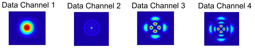
a MDM, each mode is considered as an independent channel transmitting

separate signals, as shown in Figure 1.2. Each signal is mapped to a specific

mode, and a multiplexer at the transmitter couples all the signals in a single

Data Channel 1 _{Data Channel 2} Data Channel 3 Data Channel 4

Figure 1.2: Four data channels are mapped to four different modes in a Mode

Division Multiplexing system.

1.4

Thesis Overview

The focus of the thesis is to conduct a study of modes in gradient-index

fibers and to simulate their creation using MATLAB. In chapter 2, a theory

on transverse modes in step-index and gradient-index multi-mode fibers is

given. The chapter explains the geometry of these two types of fibers and

gives the equation for the electric field in each type. In chapter 3, a detailed

study of mode creation is conducted and the results are shown. Chapter 4

is an extension of chapter 3 where phase noise is added in the creation of

modes and the results are shown.

1.4.1

Previous Related Work

In 2005, a technique to compensate for multi-mode fiber dispersion by

adap-tive optics was reported by Shen et al. [14]. In this technique a Spatial Light

is accomplished by estimating ISI at the receiver side, and this information

is fed back to the transmitter, which adjusts the SLM in order to minimize

ISI. This loop continues until the minimum ISI is reached.

In 2011, yet another technique that uses an SLM for mode creation

was reported by Stepniak et al. [8]. In this technique, however, the SLM

takes on two values, 0 or π. Instead of utilizing ISI to adjust the SLM as in

the previous work did, the pattern applied to the SLM corresponds to the

target mode desired at the receiver. This method only works with a type of

gradient-index multi-mode fiber modes, namely Laguerre polynomial-based

modes, since the phase of these modes exhibits a π phase shift.

1.4.2

Advancement of the State of the Art by the

Cur-rent Thesis

In this thesis, we have extended the work by Stepniak et al. [8] by studying

the modal cross-talk in gradient-index multi-mode fibers. This is an

impor-tant study because modes are not created with 100%. Some of the power

is coupled into other modes which causes the problems of modal dispersion.

Knowing the power coupling between modes can help when designing a

net-work that can only tolerated a given modal dispersion.

by up to 23% is proposed. Finally, the noise of the SLM is considered in the

process of creating gradient-index multi-mode fibers. This is a valid study

because opto-electronics components of the SLM will inherently introduce

Chapter 2

Mode Theory in Multi-mode

Fibers

2.1

Geometry of Fibers

An optical fiber is a cylindrical dieletric waveguide that consists of an inner

region, namely core, of high refractive index surrounded by an outer region,

namely cladding, of lower refractive index as shown in Figure 2.1. Two

types of multi-mode fibers will be studied in this section: step-index fibers

Figure 2.1: Refractive index profile in: (a) multi-mode step-index fiber, (b)

2.2

Multi-mode Step-index Fibers

In multi-mode step-index fibers, the core fills the whole region r _≤ a with

a refractive index n1, and the cladding region r > a is of index n2. The

normalized index difference of a multi-mode step-index fiber is expressed as

[4][5]

∆ = n

2 1−n22

2n2 1

≈ n1_n−n2

1

. (2.1)

In most commercial fibers, n1 ≈ n2, and thus the appromimation

in Eq. (2.1) . This condition is called the weak-guidance condition. The

numerical aperture (NA) defines the acceptance cone in which the incident

ray will experience total internal reflection. The NA is given by

N A=

q

n2

1−n22 =n1

√

2∆. (2.2)

2.2.1

Electric Field in Multi-mode Step-index Fiber

Given the weak-guidance approximation,linearly polarized (LP) modes arise

in optical fibers [7]. These modes consist of an x-poloarized electric

com-ponent and a y-polarized magnetic comcom-ponent [5]. The field comcom-ponents

are

and

H=Hy(r, θ,z)aˆy =Hy0(r, θ)exp(-iβz)aˆy (2.4)

where r is the radius from the center of the core and θ the azimuthal angle.

Using Maxwell’s equations and Helmholtz equations

∇2_E+k2_{E= 0 (2.5)}

and

∇2_H+k2_{H= 0 (2.6)}

where the transverse Laplacian

∇2

≡ ∂

2

∂x2 +

∂2

∂y2, (2.7)

and assuming tranverse variation in both r and θ [5], the wave equation in

either region is given by

∂2Ex

∂r2 +

1 r ∂Ex ∂r + 1 r2

∂2Ex

∂θ2 +β

2

tEx = 0 (2.8)

where

• β_t2 = (n2₁k₀2₋β2) is the transverse propagation constant

• k0 = 2_λπ₀ is the free space wave number

Assuming the solution for Ex to be a seriers of modes separable in r,

θ, and z, the solution Ex takes on a form of

Ex =

X

i

Ri(r)Φi(θ)exp(-iβiz). (2.9)

Each term Ex =RΦexp(-iβiz) in Eq. (2.9) is itself a solution to Eq.

(2.8), and can be substituted in Eq. (2.8) to obtain

r2 R

d2_R

dr2 +

r R

dR

dr +r

2_β2

t =−

1 Φ

d2_Φ

dθ2. (2.10)

Since r and θ are indepentent, it follows that both sides of Eq. (2.10)

are equal to a constant, namely l2, and are separable into

d2_Φ

dθ2 +l

2_{Φ = 0 (2.11)}

and

d2_R

dr2 +

1 r

dR

dr + [β

2

t −

l2

r2]R = 0. (2.12)

The solutions to Eq. (2.11) and Eq. (2.12) are

Φ(θ) =

      

cos(lθ+α)

sin(lθ+α)

and

Ex =

      

Jl(ur_a)

Kl(w_ar)

(2.14)

respectively, where:

• Jl and Kl are ordinary Bessel functions of first kind of order l and

modified Bessel function of first kind of order l, respectively,

• u=apn2

1k20−β2 and w=a

p

β2_−n2

2k20 are normilized transverse

phase and attenuation constants, repectively.

The complete electric field Elm and magnetic field Hlm are

Elm =

      

Jl(r_aul,m)cos(lθ)exp(−iβz), r≤a

Jl(ul,m)

Kl(wl,m)Kl(w

r

a)cos(lθ)exp(−iβz), r > a

(2.15)

Hlm =

      

Jl(r_aul,m)cos(lθ)exp(−iβz), r ≤a

Jl(ul,m)

Kl(wl,m)Kl(w

r

a)cos(lθ)exp(−iβz), r > a

(2.16)

where l and m designate the azimuthal mode number and the radial mode

2.2.2

Eigenvalues of Multi-mode Step-index Fibers

Some conditions, such as the core radius, the operating wavelength, and the

index difference between core and cladding, have to be met for modes to be

excited in the fiber, and these parameters have to be set so that the

boundary condition is met: the electric and magnetic fields must be

continuous at the core-cladding boundary r =a. This condition is called

the characteristic equationor dispersion relation. In weakly guiding

fibers, this condition is approximated by the condition that Eq. (2.14) be

continous at r =a, and is satisfied when

Jl−1(u) Jl(u)

=₋w

u

Kl−1(w)

Kl(w)

(2.17)

where

V2 =u2+w2, (2.18)

and V is the V-parameter given by V = 2π_λa

0N A. The solution to Eq.

(2.17) yields values for u and w for which the given mode is excited.

However, this equation is a transcendental function and cannot be solved

using the algebraic methods. The equation can be rewritten as

Jl−1(u) Jl(u)

+ w

u

Kl−1(w)

Kl(w)

= 0 (2.19)

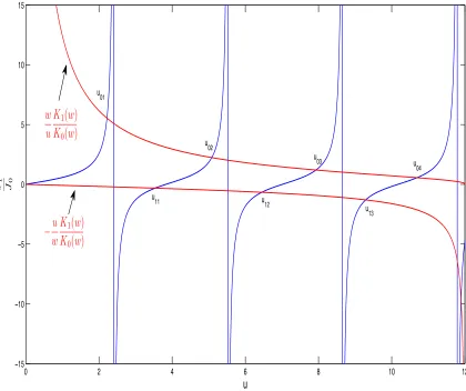
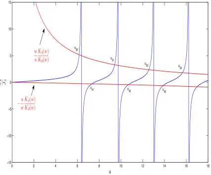
equation. A graphical method is another way of solving this equation. The

right-hand side and the left-hand side of Eq. (2.17) are ploted against u

and their intersections yield the values of u and w given V. Figure 2.2

0 2 4 6 8 10 12 −15 −10 −5 0 5 10 15 w u

K1(w) K0(w)

−_wuK_K1(w)

0(w)

J 1 J 0 u u 01 u 11 u 02 u 12 u 03 _u 04 u 13

Figure 2.2: Graphical solution for multi-mode step-index E0,m and E1,m.

0 2 4 6 8 10 12 14 16 18 −15 −10 −5 0 5 10 15 w u

K4(w) K3(w)

−_wuK_K4(w)

3(w)

J 4 J 3 u u 30 u 31 u 32 u 33 u

41 u₄₂ u₄₃

Figure 2.3: Graphical solution for multi-mode step-index E3,m and E4,m.

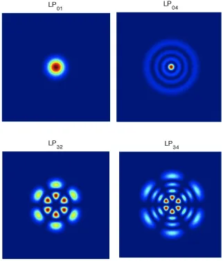
2.2.3

Intensity Profiles of some Step-index Modes

The intensity profile of a step-index multi-mode fiber modes is given by

Il,m=|El,m|2. (2.20)

Replacing the values of ul,m and wl,m obtained from the graphical solution

of Eq. (2.17) into Eq. (2.15), and setting z = 0, the intensity plots of E01,

2.3

Multi-mode Gradient-index Fibers

Figure 2.5: Power-law refractive-index profile n(r).

In gradient-index fibers, the core does not have a uniform refractive index

as it is the case in step-index fibers. The refractive index in the core

decreases with increasing radial distance from the center of the core. The

slowly varying index criterion, used in geometrical optics, is used in

gradient-index fibers to overcome the diffraction and scattering effects that

occur when the refractive index abruptively changes [9]. This criterion is

defined as

|λdn/dx

n |<< 1 (2.21)

and is interpreted as follows: the variation in refractive index that occurs

refractive index in core region.

The most used refractive index profile in gradient-index fibers is

parabolic, i.e, the light takes on a sinusoidal path as it propagates down the

fiber as shown in Figure 2.1. The advantage of this profile over a

step-index profile is that the modal dispersion is minimized [9]. The

parabolic refractive index profile is given by

n2(r) = n2₁[1₋2∆(r

a)

p

] (2.22)

where

• ∆ = n21−n22

2n2

1 ≈

n1−n2

n1

• p, the grade profile parameter, determines the steepness of the profile

• n1 highest refractive index at the center of the core

• n2 refractive index in the cladding

The grade profile parameter of p= 2 is used for best reduction of modal

2.3.1

Electric Field in Multi-mode Gradient-index

Fibers

In gradient-index fibers, Maxwell’s equations and Helmholtz equations are

given by

∇2_{E+ (n}2_(r)k2

0 −β2)E = 0 (2.23)

and

∇2

H+ (n2(r)k₀2₋β2)H= 0. (2.24)

To solve these equations, a similar method as in step-index fibers is used.

By substituting one term of Eq. (2.9) into Eq. (2.23), the wave equation for

a gradient-index fiber becomes

d2_R(r)

dr2 +

1 r

dR(r)

dr + [n

2_(r)k2 0 −β

2

− l

2

r2]R(r) = 0 (2.25)

and

d2Φ

dθ2 +l

2_{Φ = 0. (2.26)}

Eq. (2.26) is the same as Eq. (2.11) and yields the same solution. Eq.

(2.25), however, is different from Eq. (2.12) in that n2_{(r) is not a constant.}

However, a qualitatively similar function to a Bessel function results as a

Substituting Eq. (2.22) with p= 2 in Eq. (2.25) yields a Laguerre- or

Hermite-Gaussian function. In other cases where p₆= 2, the WKB method,

invented by Kramers and L. Brillouin, is used to approximate the solution

[9]. The complete electric field in a gradient-index fiber using the Laguerre

form solution is

Elm=

       Ll

m−1(ρ2)ρlexp(

−ρ2

2 )cos(lθ)exp(−iβz), r≤a

Jl(ul,m)

Kl(wl,m)Kl(w

r

a)cos(lθ)exp(−iβz) r > a

(2.27)

where

ρ=

s

k0n1

√ 2∆

a r (2.28)

and the Laguerre function is

Ll_n=

n X

s=0

(n+l)!(₋1)s_ρ2s

(l+s)!(n₋s)!s!. (2.29)

2.3.2

Orthogonality of Gradient-index Fiber Modes

The coefficient that defines how good two modes of electric fields El1,m1 and

El2,m2 overlap is defined as an overlap integral given by

η= ∞ R −∞ ∞ R −∞

El1,m1(x, y)E ∗

l2,m2(x, y)dxdy

2 ∞ R −∞ ∞ R −∞

E_l1,m1(x, y)

2 dxdy ∞ R −∞ ∞ R −∞

E_l2,m2(x, y)

2 dxdy

In polar coordinates, Eq. (2.30) is η= 2π R 0 ∞ R 0

El1,m1(r, θ)E ∗

l2,m2(r, θ)rdrdθ

2 2π R 0 ∞ R 0

E_l1,m1(r, θ) 2 rdrdθ 2π R 0 ∞ R 0

E_l2,m2(r, θ)

2 rdrdθ

. (2.31)

Substituting the electric fields in Eq. (2.31) by their respective

expressions in Eq. (2.15), the numerator becomes

2π Z 0 ∞ Z 0 Ll1

m0

1(ρ

2 r2)Ll2

m0

2(ρ

2

r2)(ρr)l1+l2_e−ρ2r2_cos(l

1θ)cos(l2θ)rdrdθ

2

(2.32)

where m0_n =mn−1

By substituting ρ2_r2 _{by ϕ, rdr =} 1

2ρ2dϕ, Eq. (2.32) becomes

1 4ρ4

2π Z 0 ∞ Z 0 Ll1

m0₁(ϕ)L

l2

m0₂(ϕ)ϕ

l₁₊l₂

2 e−ϕcos(l₁θ)cos(l₂θ)dϕdθ

2

(2.33)

Sinceϕ and θ vary independently, Eq. (2.33) can be written as

1 4ρ4

2π Z 0

cos(l1θ)cos(l2θ)dθ

∞

Z

0 Ll1

m0

1(ϕ)L

l2

m0

2(ϕ)ϕ

l1+l2

2 e−ϕdϕ

2

The Laguerre functions are orthogonal over [0,_∞) with respect to the

weighting function xl_e−x_{, i.e,}

∞

Z

0 Ll1

m1(x)L

l2

m2(x)x

l₁₊l₂

2 e−xdx=

      

0, m1 6=m2 and l1 =l2

(m+l)!

m! , m1 =m2 and l1 =l2

(2.35)

Additionally, cosine functions are also orthogonal [16], as in Eq. (2.36),

π Z

−π

cos(l1x)cos(l2x)dx=

      

0, l1 6=l2

1, l1 =l2.

(2.36)

Given Eq. (2.35) and Eq. (2.36), it follows that the power coupling

between two modes of electric fields El1,m1 and El2,m2 is

η =       

0, m1 6=m2 orl1 6=l2

1 m1 =m2 and l1 =l2

(2.37)

Modes of identical azimuthal and radial mode numbers completely

overlap, and modes of different azimuthal mode number or radial mode

2.3.3

Intensity Profiles of some Gradient-index

Modes

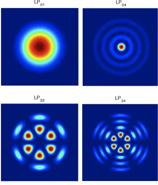
The intensity profile of a gradient-index multi-mode fiber modes is given by

Il,m=|El,m|

2

. (2.38)

Figure 2.6 shows the intensity plots of E01,E04, E32, and E33 in a

Chapter 3

Transverse-Mode Phase Masks

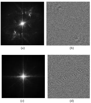
The result of Fourier-transforming a signal that changes amplitude and

phase in the near-field shows the change of amplitude and phase in the

far-field. Figure 3.1 shows two images in the near-field and Figure 3.2

shows their corresponding amplitude and phase variations in the far-field.

The spectral amplitude and the spectral phase have been studied to see

which preserves more information about the original signal. In some

situations, only partial Fourier domain information is available or desired

over the other to reconstruct the original signal. It has been shown that

phase-only holograms, where the phase is recorded and the amplitude is

assumed to be unity, the signal is reconstructed with more features of the

original signal than the reconstructed signal from an amplitude-only

zero [8][13]. Figure 3.3 shows this interesting finding. The phase of Image

A is used in the reconstruction of Image B, while the phase of Image B is

used in the reconstruction of Image A. We can see that the spectral phase

carries more information about the original signal than the spectral

amplitude. It follows that using a phase-only spatial light modulator, fiber

modes can be reconstructed with minimal error.

                                                                                                                                 (a)     (b)  

                                                                                                             (c)     (d)  

Figure 3.2: In the far-field (a) Image A amplitude, (b) Image A phase, (c)

!! ! !

!!!!!!!!!!!!!!!!!!!!!!!!!!!!!!!!!!(a)!! (b)!

Figure 3.3: Reconstructed Images (a) Amplitude of Image A with phase of

3.1

Construction of Fiber Modes using a

Spatial Light Modulator

Figure 3.4: Construction of Fiber Modes using a Spatial Light Modulator.

Consider a 4-f optical setup shown in Figure 3.4. A spatial light modulator

(SLM) is placed in the Fourier plane of the first lens. The electric field Esi

incident upon the SLM is the Fourier transfom of the signal originating

Esi(fx, fy)∝F T{Ei}=

∞

Z Z

−∞

Ei(x1, y1)ej2π(fxx1+fyy1)dx1dy1 (3.1)

where

• Ei is the electric field from the input fiber

• fx = _λfx and fy = _λfy are the spatial frequencies

• (x, y) is the coordinate system in the Fourier plane

• λ is the signal wavelength

• f is the focal distance of the lens

• F T is the Fourier transform symbol

The incident field upon the second lens is the product of Esi and the

transfer function of the SLM T(fx, fy). The second lens performs another

Fourier transform of the incident signal and focuses the light into the

transmission fiber. Thus, the electric field E0 incident upon the

transmission fiber is given by [10]

Eo(x2, y2)∝F T{T(fx, fy)Esi(fx, fy)}=

∞

Z Z

−∞

T(fx, fy)Esi(fx, fy)ej2π(x2fx+y2fy)dfxdfy

where(x2, y2) is the coordinate system in the plane of the transmission fiber.

Although the field propagating out of the input fiber is usually

considered to be Gaussian, it can be assumed to be an impulse function

δ(x1, y1) without much compromise [12]. With this assumption, it follows

that Esi ∝F T{δ(x1, y1)}= 1. In turn, Eq. (3.2) becomes

Eo ∝F T{T(fx, fy)}=

∞

Z Z

−∞

T(fx, fy)ej2π(x2fx+y2fy)dfxdfy. (3.3)

At the transmission fiber, to excite a specifc mode, the incident electric

field Eo(x2, y2) has to match or overlap with the mode to be excited. The

quality of overlap is calculated with an overlap integral given by [11]

η= |

RR

Eo(x2, y2)EM∗ (x2, y2)dx2dy2|2

RR

|Eo(x2, y2)|2dx2dy2

RR

|EM(x2, y2)|2dx2dy2

(3.4)

where η is the power coupling coefficient (P C) and EM is the electric field

of the mode to be excited.

The maximum valueη takes on is 1 and this happens when Eo =EM,

i.e., Eo and EM completely overlap. It is then evident that in order to

excite a given mode EM, the transfer function of the SLM has to be the

T(fx, fy) =F T−1{EM(x2, y2)}=

∞

Z Z

−∞

EM(x2, y2)e−j2π(fxx2+fyy2)dx2dy2.

(3.5)

3.2

Unit Amplitude

As discussed earlier, the spectral phase of a signal carries more

information about the original signal than the spectral amplitute. Using a

phase-only spatial light modulator and assuming that the amplitude of the

light field reaching the front end of the SLM is a unit over the transmissive

region of the SLM, a desired mode is excited in the transmission fiber given

that the transfer function of the SLM is equal to the spectral phase of the

desired mode transform,

˜

T(fx, fy) =

T(fx, fy) |T(fx, fy)|

. (3.6)

3.2.1

Results

This section shows the results of constructed gradient fiber modes using the

setup shown in Figure 3.4. Figure 3.5 and Figure 3.6 shows how well

modes are created and the cross-talk with other modes. Mode E0,1 is

with mode E0,4 with a cross-talk coefficient of approximately 1.7x10−5. The

cross-talk coeffiencient is defined as the power coupling between a mode

and and another mode other than itself. Mode E3,2 has a power coupling of

approximately 8.8x10−5, and a cross-talk coefficient with mode E2,3 of

approximately 0.2x10−5.

0.00E+00   5.00E-­‐06   1.00E-­‐05   1.50E-­‐05   2.00E-­‐05   2.50E-­‐05  

E0,1   E0,4   E3,2   E2,3  

η  

Power  Coupling  &  Modal  Cross-­‐talk  

E0,1  

0.00E+00   1.00E-­‐05   2.00E-­‐05   3.00E-­‐05   4.00E-­‐05   5.00E-­‐05   6.00E-­‐05   7.00E-­‐05   8.00E-­‐05   9.00E-­‐05   1.00E-­‐04  

1   2   3   4  

η  

Power  Coupling  &  Modal  Cross-­‐talk  

E3,2  

As the results show, using a unit amplitude across the transmissive area

of the SLM and using the phase signal of the target mode, the modes are

created at the output fiber with very little power coupling. The following

sections focus on improving this technique.

3.3

Optimal Aperture

3.3.1

Abbe’s Theory

Consider the 4-f optical system in Figure 3.7. Each point in the Fourier

plane (x, y) of the first lens corresponds to a spatial frequency and

amplitude. Abbe’s theory states that to reconstruct the image of the

original object, as many diffraction orders as possible must be recombined

for higher quality image of the object [13]. These diffraction orders

correspond to spatial frequencies. The second lens recombines the spatial

frequencies to reconstruct the image in the object plane (x2, y2). The

spatial frequencies (fx, fy) in the Fourier plane are related to (x, y) system

Figure 3.7: Abbe’s Theory of Imaging.

fx =

x

λf (3.7)

and

fy =

y

λf. (3.8)

where λ is the light wavelength and f is the focal distance of the first and

3.3.2

Aperture Diameter Optimization

The assumption that the light field reaching the SLM has a constant

amplitude across the transmissive area of the SLM requires that higher

frequencies be filtered out for maximum power coupling. To understand

this reasoning, lets consider the transfer function T of the SLM to be the

inverse Fourier transform of EM with both amplitude and phase. Here we

assuming that the SLM is configured to modulate amplitude and phase. If

T is applied to the SLM, the resulting electric fieldEo at the input on the

transmission fiber completely overlaps with EM, i.e., η= 1. However, it is

evident from Figure 3.8 that not all the spectral frequencies have the same

amplitude; there is a maximum frequency passed which the amplitude

Figure 3.8: Frequency Component of Mode E04.

However, if the amplitude component of the transfer function is

assumed to be constant across the sprectrum, higher order frequencies have

to be filtered out in order to achieve a high η, otherwise the resulting strong

interferance at high frequencies will cause the power coupling η to be much

less than 1. This is the case of Section 3.2. It follows that an aperture is

required to block higher frequencies, and the resulting setup is shown in

diameter that will result in maximum η.

SLM

Lens

Lens

Aperture

Figure 3.9: An aperture is placed in front of SLM to block high frequencies.

We calculate the optimal aperture diameter by varying the maximum

frequency allowed through the aperture and recording the resulting power

coupling. Eq. (3.7) and Eq. (3.8) shows the relationship between (x, y)

coordinates in the Fourier plane and their corresponding spatial

frequencies. Figure 3.10 and Figure 3.11 show the change of η with

optimal diameter at which the highest power coupling is reached for any

given mode. For example, for mode E0,4, the maximum frequency, for both

fx and fy, at which the highest power coupling of approximately 0.8 is

0.115mm−1. Using Eq. (3.8) where the focal distance f = 20cm and the

wavelength λ= 850nm, we calculate the corresponding optimal diameter of

0 0.05 0.1 0.15 0.2 0.25 0.3 0.35 0.4 0.45 0

0.1 0.2 0.3 0.4 0.5 0.6 0.7 0.8 0.9 1

Spatial Frequency [mm−1]

η

E_0,4 E_0,5 E_0,6 E_0,7

Highest

Figure 3.10: Change of η with respect to the highest allowed frequency for

0 0.05 0.1 0.15 0.2 0.25 0.3 0.35 0.4 0.45 0

0.1 0.2 0.3 0.4 0.5 0.6 0.7 0.8 0.9 1

Spatial Frequency [mm−1_]

η

E_1,4 E_1,5 E_1,6 E_1,7

Highest

Figure 3.11: Change of η with respect to the highest allowed frequency for

With an optimal aperture in place, we have a new transfer function of

the system optimal aperture-SLM, and is

˜

T(fx, fy) =

T(fx, fy) |T(fx, fy)|

.δ p

f2

x +fy2

fmax ! (3.9) where δ p f2

x +fy2

fmax ! =        1, √ f2

x+fy2

fmax ≤1

0, √

f2

x+fy2

fmax >1

(3.10)

and fmax is the maximum frequency allowed through the aperture.

3.3.3

Results

As we can see in Figure 3.12 and Figure 3.13, the power coupling

significantly increases for angular-independent and angular-dependent

0.00   0.10   0.20   0.30   0.40   0.50   0.60   0.70   0.80   0.90   1.00  

E0,1   E0,4   E3,2   E2,3  

η  

Power  Coupling  &  Modal  Cross-­‐talk  for  Mode  E

Op1mal  Aperture   Unit  Amplitude  

E

Figure 3.12: Power Coupling and Modal Cross-talk for Mode E0,1:

0.00   0.10   0.20   0.30   0.40   0.50   0.60   0.70   0.80   0.90   1.00  

E0,1   E0,4   E3,2   E2,3  

η  

Power  Coupling  &  Modal  Cross-­‐talk  for  Mode  E

Op1mal  Aperture   Unit  Amplitude  

E

Figure 3.13: Power Coupling and Modal Cross-talk for Mode E3,2:

3.4

Optimal Inner Aperture Block

This section investigates the impact of an aperture block at the center of

the aperture for the purpose of increasing the power coupling. As it was

shown in the previous section, the use of aperture is based on the fact that

higher frequencies do not exist in the spectrum of the mode, i.e., higher

frequencies have little or no amplitude. In Figure 3.14, far-field intensity

profiles of four modes are shown. It is the property of Laguerre-based

modes that they are invariant to the the Fourier transform [8]. As we can

see in the figure, lower frequencies also do not exit in the spectrum of the

modes, and as a result there is a minimum frequency under which the

amplitude becomes zero. It is important to note that this is true for

E

E

E

E

Min Max

The intensity at the center of the mode is minimal

Figure 3.14: Lower frequencies do not exist in the spectrum of

angular-dependent modes.

It follows that by placing an aperture block to block lower frequencies

will lead to an increase in power coupling. Additionally, the optimal size of

the block that yeilds the highest increase in power coupling must be

utilized. The process of determining the optimal diameter of the inner

aperture block is similar to the one used to determine the optimal aperture

diameter: by varying the minimum frequency allowed throught the aperture

(which is equivalent to varying the maximum frequency blocked by the

inner aperture block), the power coupling is recorded, and the optimal

frequency at which the power coupling is highest. Figure 3.15 shows the

setup of the inner aperture block and Figure 3.16 shows the optimization

process of the inner aperture block.

Inner Aperture Block

Figure 3.15: Setup with Inner Aperture Block: An inner aperture block is

Figure 3.16: Change of η with respect to the lowest allowed frequency for

angular-dependent and angular-independent modes.

With an optimal aperture and an inner aperture block in place, we have

a new transfer function of the system optimal aperture-inner aperture

˜

T(fx, fy) =

T(fx, fy) |T(fx, fy)|

.δ p

f2

x +fy2

fmax

!

.γ _pfmin

f2

x +fy2

!

(3.11)

where

γ _pfmin

f2

x +fy2

! =       

1, √fmin

f2

x+fy2 ≤

1

0, √fmin

f2

x+fy2

>1

(3.12)

and fmin is the minimum frequency not blocked by the inner aperture block.

3.4.1

Results

Figure 3.17 and Figure 3.18 show the results of using an optimized inner

aperture block. We can see that by utilizing an inner aperture block, the

power coupling significantly increases in this way:

• As previously noted, only angular-dependent modes will experience a

power coupling increase by the use of an inner aperture block.

• The percentage power coupling increase increases with increasing

azimuthal mode number.

• The percentage power coupling increase decreases with increasing

0   5   10   15   20   25   30  

E0,1   E1,1   E2,1   E4,1   E6,1   E8,1   E10,1  

Percentage  Increase  -­‐  Increasing  Azimuthal  Number  

Figure 3.17: Percentage Increase in Power Coupling: Increasing Azimuthal

0   5   10   15   20   25   30  

E10,1   E10,2   E10,3   E10,4   E10,5  

Percentage  Increase  -­‐  Increasing  Radial  Number  

Figure 3.18: Percentage Increase in Power Coupling: Increasing Radial Mode

Chapter 4

Far-field Phase Noise

Thus far, in the creation of modes using far-field phase information, we

have considered an noiseless SLM, i.e., the SLM transfer function is equal

to the phase of the target mode, with no noise considered. However, in

reality this noise exists and is due to the effect of opto-electrical

components of the SLM. This chapter will explore the effect that the SLM

noise has on the creation of modes.

4.1

SLM Noise

In this section, we consider the SLM noise φ(fx, fy) to be a White Gaussian

noise of probability density function defined as

ξ= 1

σ√2πe

−f 2

x+fy2

where σ is the standard deviation of the noise.

With the SLM noise considered, the total transfer function becomes

˜

T(fx, fy) =

φ(fx, fy) +

T(fx, fy) |T(fx, fy)|

.δ p

f2

x +fy2

fmax

!

.γ _pfmin

f2

x +fy2

!

(4.2)

The signal to noise ration (SNR), which defines the level of the phase to

the level of the noise, is defined as

snr= 10 logP(fx, fy)

φ(fx, fy)

, (4.3)

where

P(fx, fy) =

T(fx, fy) |T(fx, fy)|

(4.4)

4.2

Effect of SLM noise on creation of

modes

Using the transfer function defined in Eq. 4.2, Figure 4.1 shows the creation

of modes as a function of SNR. As we could have predicted, a higher SNR

SNR = 0 SNR = 5 SNR = 10 SNR = 15

E

:

E

:

E

:

Figure 4.1: Effect of SLM noise of mode creation.

Figure 4.2 shows the impact of SNR on the power coupling. We see

that a phase-to-noise ratio of approximately 30dB is sufficient to achieve

maximum power coupling for modes

E0,1, E0,4, E4,1, E4,4, E8,1, E8,4, E12,1, E12,4. It is also important to notice that

reconstruct modes with maximum power coupling holds true independently

of the azimuthal or radial mode number.

Chapter 5

Concluding Remarks

This thesis investigated the creation of gradient-index fiber modes, first by

studying the electromagnetic fields of light in step-index and gradient-index

multi-mode fibers, and secondly by simulating the creations of modes using

MATLAB utilizing different techniques with the goal to maximize the

power coupling between the created mode and the desired mode.

We first reproduced a previous work by Stepniak et al. [8] and extended

the work by introducing an inner aperture block in the far field, which

resulted in an increase of power coupling of up to 23%. We examined this

technique for angular-depend and angular-independent modes and found

that this technique increases the power coupling for angular-dependent

modes only. We also reported that the power coupling increases with

mode number.

Finally, we investigated the effect of SLM noise to the creation of

modes. This is an important study because SLM noise is an inherent

property that needs to be considered in the creation of modes. We reported

that an approximate of 30dB of SNR is necessary to create modes with

Bibliography

[1] J. S. Lim A. V. Oppenheim and S.R. Curtis. Signal synthesis and

reconstruction from partial fourier domain information. Journal of the

Optical Society of America, 73:1413–1420, November 1983.

[2] M.J. Adams. Fundamentals of Optical Fibers. Wiley-Interscience, 2nd

edition, 1981.

[3] Vladimir. Kahn Joseph M. Boyd Stephen. Alon, Elad. Stojanovi and

Mark Horowitz. Equalization of modal dispersion in multimode fiber

using spatial light modulator. Global Telecommunications Conference,

2:1023–1029, 2004.

[4] K. G. Birch. Spatial filtering in optical data-processing. Rep. Prog.

Phys., 29:1265–1314, September 1972.

[5] David M. Bressoud. A Radical Approach to Real Analysis. The

[6] John A. Buck. An Introduction to Optical Waveguide.

Wiley-Interscience, 2nd edition, 2004.

[7] Joel Carpenter and Timothy D. Wilkinson. Characterization of

multimode fiber by selective mode excitation. Optics Letters, 30(10),

May 2012.

[8] W. Thomas Cathey. Optical Information Processing and Holography.

Wiley-Interscience, 1989.

[9] L. Maksymiuk G. Stepniak and J. Siuzdak. Binary-phase spatial light

filters for mode-selective excitation of multimode fibers. Journal of

Lightwave Technology, 29(13):1980–1987, July 2011.

[10] D Globe. Weakly guiding fibers. Applied Optics, 10(10):2252–2258,

October 1971.

[11] Keang-Po Ho Joseph M. Kahn and Mahdieh Bagher Shemirani. Mode

coupling effects in multi-mode fibers. In Optical Fiber Communications

Conference, March 2012.

[12] D. G. Cunningham L. Raddatz, I. H. White and M. C. Nowell.

Experimental and theoretical study of the offset launch technique for

the enhancement of the bandwidth of multimode fiber links. Journal of

Lightwave Technology, 16(3):324–331, March 1998.

[13] Alan V. Oppenheim and Jae S. Lim. The importance of phase in

[14] Bahaa E. A. Saleh and Malvin Carl Teich. Fundamentals of Photonics.

Wiley-Interscience, 1st edition, 1991.

[15] Joseph M. Kahn Xin Shen and Mark A. Horowitz. Compensation for

multimode fiber dispersion by adaptive optics. Journal of Lightwave

Technology, 30, November 2005.

[16] X. Zhao and F.S Choa. Demonstration of 10-gb/s transmission over

1.5-km-long multimode fiber using equalization techniques. IEEE

Appendix A

MATLAB Simulation of

Step-Index Multi-Mode Fiber

Modes

• Calculate the V number based on the fiber and light properties (fiber

core radius, numerical aperture and light wavelength)

• Define eigenvalue u as a vector of maximum value V

• Calculate eigenvalue w based on Eq. 2.18

• Define each term in Eq. 2.17 depending on the mode to be created

• Graphical method

Below is an example of a MATLAB simulation code and the

resulting graphical solution for mode of azimuthal mode number

4

– The intersections between the two plots are solutions to

eigenvalue u. The first intersection isu4,1, the second is u4,2, and

so on.

• Numerical method

– Using MATLAB built-in functions, find the root of Eq. 2.19

• Using Eq. 2.17, calculate w

• Use Eq. 2.15 and Eq 2.20, calculate the electric field of the mode

and and its intensity, respectively.

Light Properties

lambda = .85; %wavelength[microns]

k = 2*pi/lambda; %wave number

Fiber Properties

n1 = 1.46; %refractive index of the fiber core

delta = 0.0178; %normalized index difference

na = n1*sqrt(2*delta); %numerical aperture

V Parameter

v = 20; 2*pi*r*na/lambda;

Eigenvalues

u = 0:.0001:v;

w = sqrt(v.^2 - u.^2);

Bessel Functions for use in Eq. 2.16

j4 = besselj(4, u);

j3 = besselj(3, u);

k4 = besselk(4, w);

k3 = besselk(3, w);

Plotting for graphical solution

plot(u, j4./j3, ’-b’, ’LineWidth’, 1.1); hold on;

plot(u, -(u./w).*(k4./k3), ’-r’, ’LineWidth’, 1.1);

text(0.5, -6, ’$$-\frac{u}{w}\frac{K_4(w)}{K_3(w)}$$’, ’interpreter’, ...

’latex’, ’Color’, ’r’, ’fontsize’,25);

ylabel(’$$\frac{J_4}{J_3}$$’,’interpreter’,’latex’, ’fontsize’, 25);

xlabel(’u’, ’fontsize’,25);

axis([0 v -30 30])

Figure A.1: Graphical solution to eigenvalue equation. The solution is the