https://doi.org/10.5194/angeo-36-47-2018 © Author(s) 2018. This work is distributed under the Creative Commons Attribution 4.0 License.
Communica
tes
Multi-scale analysis of compressible fluctuations in the solar wind
Owen W. Roberts1, Yasuhito Narita2, and C.-Philippe Escoubet1
1ESA/ESTEC SCI-S, Keplerlaan 1, 2201 AZ, Noordwijk, the Netherlands
2Space Research Institute, Austrian Academy of Sciences, Schmiedlstr. 6, 8042 Graz, Austria
Correspondence:Owen W. Roberts ([email protected])
Received: 12 October 2017 – Revised: 9 November 2017 – Accepted: 24 November 2017 – Published: 12 January 2018
Abstract.Compressible plasma turbulence is investigated in the fast solar wind at proton kinetic scales by the combined use of electron density and magnetic field measurements. Both the scale-dependent cross-correlation (CC) and the re-duced magnetic helicity (σm) are used in tandem to
deter-mine the properties of the compressible fluctuations at pro-ton kinetic scales. At inertial scales the turbulence is hypoth-esised to contain a mixture of Alfvénic and slow waves, char-acterised by weak magnetic helicity and anti-correlation be-tween magnetic field strengthBand electron densityne. At
proton kinetic scales the observations suggest that the fluc-tuations have stronger positive magnetic helicities as well as strong anti-correlations within the frequency range studied. These results are interpreted as being characteristic of either counter-propagating kinetic Alfvén wave packets or a mix-ture of anti-sunward kinetic Alfvén waves along with a com-ponent of kinetic slow waves.
Keywords. Interplanetary physics (MHD waves and turbu-lence)
1 Introduction
The solar wind is a magnetised collisionless plasma outflow-ing from the Sun. Measurements of several parameters show irregular fluctuations over several decades in scale (Bruno and Carbone, 2013). The dominant component of the en-ergy in these fluctuations is in the directions perpendicular to the mean magnetic field directionδB⊥δBk(Bieber et al.,
1996). However, the solar wind plasma is also weakly com-pressible with non-negligible fluctuations in magnetic field strength (δBk) and density (δn) (Tu and Marsch, 1994).
Turbulence is an inherently nonlinear process. However, there is evidence that the plasma is in a state of “critical bal-ance” (Goldreich and Sridhar, 1995). This is a state where
the nonlinear timescale and the linear timescale constantly evolve toward being equal. Therefore, even when nonlinear-ity is strong, the linear terms are of the same order and the system may retain some properties of linear wave modes; this is often termed the quasilinear premise (Klein et al., 2012). Several multi-spacecraft observations of the solar wind have revealed that the fluctuations at proton kinetic scales typi-cally have low intrinsic propagation speeds in the plasma frame. This result has been interpreted as evidence of ki-netic Alfvén waves (KAWs) (Sahraoui et al., 2010), as co-herent structures which are predominantly advected with the bulk velocity (Perrone et al., 2017), as a combination of KAW turbulence and coherent structures (Roberts et al., 2013, 2015), or as nonlinear modes where wave–wave in-teractions have broadened the dispersion relation diagram (Narita and Motschmann, 2017; Roberts et al., 2017). Kinetic slow waves (KSWs) are the kinetic counterpart of the magne-tohydrodynamic (MHD) slow mode when it develops a large perpendicular wave number, and it shares many properties with the KAW, such as a similar dispersion relation and anti-correlated fluctuations in magnetic field and density (Klein et al., 2012; Narita and Marsch, 2015). The distinct identi-fication of either KAWs or KSWs using only the dispersion relation diagram is challenging given the error in the mea-surements. This result motivates further study of the same in-terval with techniques which can distinguish between KAWs and KSWs.
func-tion of the angle between the magnetic field direcfunc-tion and the bulk flow direction giving a positive value atθBV ∼90◦and
a negative atθBV ∼0◦(He et al., 2011; Podesta and Gary,
2011). This has been interpreted as evidence of the existence of quasi-perpendicular KAWs (Howes and Quataert, 2010) in addition to quasi-parallel ion cyclotron (He et al., 2011; Podesta and Gary, 2011; Klein et al., 2014) waves. However, these observations are subject to an ambiguity as a helical sense of a wave can be opposite depending on whether the plasma wave is propagating up- or downstream; which moti-vates further analysis through an investigation of the correla-tion of the compressible fluctuacorrela-tions with one another.
Ion Bernstein waves (IBWs) exhibit positive correlations between ne and B, while KAW/KSWs both exhibit
anti-correlations (Klein et al., 2012; Zhao et al., 2014). The elec-tron density is estimated from the spacecraft potential (Ped-ersen et al., 2001; Kellogg and Horbury, 2005), which has a sufficient time resolution to study proton kinetic scales. Meanwhile, magnetic helicity can be used to differentiate between KAWs and KSWs which have opposite helicities and polarisations (Zhao et al., 2014). Typically in the solar wind, B and ne are anti-correlated on fluid scales (Howes
et al., 2012), and also down to kinetic scales (Kellogg and Horbury, 2005; Yao et al., 2011), which have been inter-preted as KSWs or pressure-balanced structures (the un-damped oblique limit of the KSWs).
2 Weakly compressible event
A data interval which was taken by the Cluster (Escoubet et al., 2001) spacecraft when they were in an interval of solar wind and which is uncontaminated from the electron fore-shock is analysed. The mean angle that the solar wind makes with the solar wind bulk flow is large (θvB>60◦) suggesting
that the plasma is not connected to the electron foreshock. Furthermore, the electric field spectrogram from the WHIS-PER (Waves of High Frequency and Sounder for Probing of Density by Relaxation) instrument (Décréau et al., 1997) is quiet, with no signatures of foreshock waves. The large value ofθvBalso allows us to neglect considering any contributions
of quasi-parallel waves (e.g. He et al., 2011) in the analysis. The mean bulk speed of the solar wind is 655±15 km s−1, the mean proton density is low 2.8±0.2 cm−3, and plasma
β=0.85±0.29. There are no interplanetary coronal mass ejections or stream interaction regions recorded at the time of the interval, and the large scale from Active Composition Explorer (ACE) data (not shown) suggests that this interval can be regarded as typical of the fast solar wind (see Roberts et al., 2015).
Magnetic field data are obtained from the Fluxgate magne-tometer (FGM) instrument (Balogh et al., 2001) sampled at 22 Hz, and electron density data are obtained by calibrating the spacecraft potential sampled at 5 Hz, which is measured
0 200 400 600 800 1000 1200 1400
2.5 3.0 3.5 4.0 4.5
5.0 Cluster 4 2004−02−29 04:10–04:34UT
0 200 400 600 800 1000 1200 1400
Time (s) 2.5
3.0 3.5 4.0 4.5 5.0 (a)
2.5 3.0 3.5 4.0 4.5 5.0
ne
(cm
−3)
7 8
9
10 11
B (nT)
B
ne
0 200 400 600 800 1000 1200 1400
Time (s) −10
−5 0 5 10
B (nT)
(b)
Bx
By
Bz
0.0 0.5 1.0 1.5 −2
−1 0 1
2ne fluctuations
0.0 0.5 1.0 1.5
kvA/Ωp
−2 −1 0 1 2
ωpla
/
Ωp KAWKSW
IBW (c)
B fluctuations
0.0 0.5 1.0 1.5
kvA/Ωp
−2 −1 0 1 2
ωpla
/
Ωp (d)
Figure 1. (a)Time series of the density (red) and the magnetic field strength (blue) fluctuations from the Cluster 4 spacecraft.(b)Time series of the magnetic field components in the GSE co-ordinate sys-tem.(c)Dispersion relation diagram of the electron density fluctu-ations(d) compressible magnetic fluctuations. Theoretical disper-sion relations for advected structures (green), KAWs (red), KSWs (cyan) and IBWs (orange) for propagation anglesθkB0=88
◦and
75◦(solid lines).
by the Electric Fields and Waves (EFW) instrument (Gustafs-son et al., 1997).
The spacecraft potential is subject to a strong spin effect at 0.25 Hz and charging effects due to different parts of the spacecraft being illuminated. To remove these fluctuations we use the method presented in Roberts et al. (2017) to con-struct an empirical model of the spacecraft charging as a function of the phase angle. This allows the fluctuations in the spacecraft potential due to solar illumination to be re-moved, leaving only fluctuations due to density fluctuations. This is effective up to 1.0 Hz, above which high-frequency spikes remain and instrumental noise also becomes signifi-cant.
In Fig. 1a the electron density ne is given in red, and
[image:2.612.309.543.63.362.2]geo-centric solar ecliptic (GSE) co-ordinates, wherexGSEpoints
from the Earth towards the Sun andzGSEpoints to the ecliptic
north.
The dispersion relation diagrams of compressible magnet-ics and density obtained from the interval used in this study are shown in Fig. 1c and d. These are derived by the appli-cation of the multi-point signal resonator technique (Narita et al., 2011), which allows the most energetic wave vectork
to be identified at each spacecraft frequencyωsc. The
corre-sponding plasma frame frequency can be obtained from the equationωpla=ωsc−k·v. Further details can be obtained in
Roberts et al. (2017). Figure 1c and d also show the theoreti-cal linear dispersion curves for the KAWs, IBWs and KSWs for plasmaβ=0.85 (ratio of thermal to magnetic pressure). A green dashed line atω=0 denotes the expectation for a static structure. The rest-frame frequencies of the fluctuations
ωpla/pshow a lot of scatter from the theoretical curves, and
the error bars are significant. Moreover, the theoretical ex-pectations for both KAWs and KSWs are very close to one another for angles close to 90◦. This motivates the analysis of the time interval with correlations and the magnetic helicity.
To obtain a multi-scale picture, we perform a cross-correlation and magnetic helicity based on wavelet analysis (Torrence and Compo, 1998), which allows the relationship between the two signals to be analysed in time and in scale (frequency).
3 Correlation and helicity analysis
3.1 Estimators
The wavelet cross-correlation is given in Eq. (1), whereene
andBeare the complex wavelet coefficients for the electron
density and the magnitude of the magnetic field respectively, while the Re denotes the real part and the asterisk denotes the complex conjugate. The value of CC varies between−1 (full anti-correlation) and +1 (full correlation). In order to com-pare the magnetic field data with the electron density data in this way, the magnetic field data are resampled at 5 Hz.
CCn,B(t, f )=
Re ene(t, f )Be∗(t, f )
|
ene(t, f )||B(t, f )e |
(1)
As a further diagnostic tool for the magnetic fluctuations, we also analyse the magnetic helicity. The magnetic helicity is the spatial rotation sense of the magnetic fluctuation about the wave vector. We use the definition in Eq. (2), where the tilde denotes the wavelet coefficients of the GSE components of the magnetic field in GSE and Im denotes imaginary parts.
σm(t, f )=
ImBey∗(t, f )Bez(t, f )
|Bey(t, f )|2+ |Bez(t, f )|2
(2)
It is important to note that this definition assumes that the wave vectorkis along−xGSE (approximately along the
flow) and also implicitly assumes Taylor’s hypothesis, i.e. that there is no temporal change. Thus, the magnetic helic-ity varies between−1 and+1 and for this definition can be regarded as being the same as polarisation (temporal rotation sense of the fluctuations with respect to the magnetic field). Thus, positive (negative) helicity is indicative of a polarisa-tion sense in the right- (left-) handed direcpolarisa-tion in the direcpolarisa-tion of electron (proton) gyration. However, an important caveat of this method is that it does not contain information about the propagation direction of the fluctuations. As such a right-hand polarised wave can give the appearance of a left-right-handed wave if the propagation direction is reversed (Narita et al., 2009).
3.2 Results
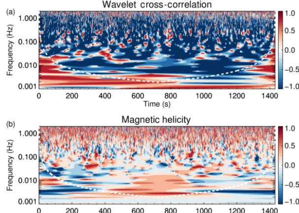
Figure 2a shows the cross-correlation spectra, where the white line denotes the cone of influence associated with the wavelet transform (Torrence and Compo, 1998); below this line the spectrum is unreliable due to edge effects. The spec-trum is dominated by anti-correlated fluctuations throughout with small regions of sporadic positive correlation peppering the spectrum. This suggests that IBWs are not present or are only present for very brief times.
Figure 2b shows the magnetic helicity spectrum. The value of the helicity shows a mix of different values on fluid scalesf ∈ [0.01,0.2]and a general increase on kinetic scales
f ∈ [0.4,2]towards a value ofσm∼0.5 near 1 Hz. At
space-craft frame frequencies offsc≥1.0 Hz and fsc≥2 Hz,
in-strumental noise becomes significant in the spacecraft poten-tial and in the magnetic field data respectively. Another im-portant issue is that of aliasing, which affects high frequen-cies and can artificially reduce the value of the helicity (e.g. Klein et al., 2014). However, in previous studies of the helic-ity, the sampling rates of magnetic field instruments is much lower than for Cluster, and the data presented here are not as strongly affected. Aliasing would be expected to signif-icantly affect frequencies above 5.5 Hz in the helicity mea-surement and 1.25 Hz for the cross-correlation; however, we are already near the instrument noise levels.
The negative cross-correlation signature and negative he-licity on fluid scales is likely to be due to MHD slow waves (Howes et al., 2012) or pressure-balanced structures (Yao et al., 2011). However, there are regions on fluid scales which have positive helicity and negative cross-correlation which could be due to a fluid-scale Alfvén wave. On ion kinetic scales, more regions of positive cross-correlation appear, but they are still less numerous than the negatively correlated re-gions, while the magnetic helicity increases and is predomi-nantly above 0.
Figure 2. (a)Wavelet cross-correlation of the electron density and magnetic field strength.(b)Magnetic helicity. The white dashed line denotes the cone of influence region where the spectrum is unreliable due to edge effects.
Table 1. Table of the thresholds used to identify different wave modes for fluid (fl) and kinetic (ki) scales.
Branch σm(fl) CC (fl) σm(ki) CC (ki)
Alfén (AW) >0,<0.5 <−0.5 >0.5 <−0.5 Slow (SW) <0,<−0.5 <−0.5 <−0.5 <−0.5 Fast (FW) >−0.05,<0.05 >0.5 >−0.3,<−0.05 >0.5
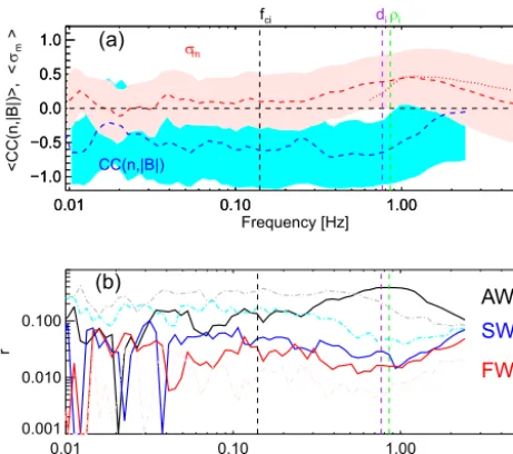
then remains at a similar value until Taylor-shifted proton scales, and then it increases before being influenced by noise near 2 Hz. The magnetic helicity is close to 0 on fluid scales and then increases at 0.5 Hz, reaching a maximum plateau at the Taylor-shifted scales (denoted by the green and purple vertical line) before decreasing. Analysis of the helicity from the search coil magnetometer (SCM) (Cornilleau-Wehrlin et al., 2003) is shown as the dotted red line in Fig. 3a. The SCM is more sensitive than FGM and is sampled at 25 Hz. The data from SCM show that the helicity is indeed lower at 2< fsc<5.5 Hz, and due to the higher sampling rate and
sensitivity, this is not an artefact of aliasing or noise. To understand the relative importance of the competing wave modes, we use the thresholds in Table 1 to find the relative occurrence rates. These thresholds are motivated by what is expected for each wave mode from linear theory (e.g. Klein et al., 2012) and assume anti-sunward propagation.
Figure 3b shows the ratiorof data points which reach the thresholds outlined in Table 1 to the total number of data points. On large scales the plasma is dominated by MHD Alfvén waves and slow waves. However, as we approach pro-ton scales, these both decrease and this method clearly iden-tifies that the dominant type of fluctuation on proton scales
is the KAW, with very few points at proton kinetic scales reaching the thresholds for KSWs or IBWs. At the highest frequencies there is a small increase in both of these wave modes; however, it is unclear whether this is true or related to the instrumental noise. It should be noted that a sunward-propagating KSW would in this case produce the same signa-ture as the KAW; therefore, in interpreting the data in Roberts et al. (2017) and Fig. 1c and d this mixture of two waves may explain the scatter seen. Moreover, even though some points in Fig. 1c and d, may agree better with the curves for IBWs as there is no significant signature in the cross-correlation, this is most likely due to wave–wave interactions between individual KAW packets or KAWs and KSWs (Narita and Motschmann, 2017; Roberts et al., 2017). It is also interest-ing to note that while the KAW dominates both other wave modes, the majority of the fluctuations do not fall into the thresholds in Table 1.
4 Conclusions
[image:4.612.46.286.372.420.2]0.01 0.10 1.00
−1.0 −0.5
0.0
0.5
1.0
0.01 0.10 1.00
Frequency [Hz]
−1.0 −0.5
0.0
0.5
1.0
<CC(n,|B|)>, <
σ m
> (a)
σm
CC(n,|B|)
fci diρi
0.01 0.10 1.00
Frequency [Hz] 0.001
0.010 0.100
r
AW
SW
FW (b)
Figure 3. (a)Mean values at each spacecraft frame frequency for the helicity (red) and the wavelet cross-correlation (blue). Light shaded areas denote 1 standard deviation, and the dashed red line denotes the helicity from the search coil magnetometer.(b)Ratio of data points meeting the thresholds to the total number of points in the interval, which are defined in Table 1. The solid lines denote the ratio of points that meet the kinetic thresholds. Lighter dotted lines denote the ratio for the fluid thresholds.
A plausible scenario is that on inertial scales the com-pressible component is dominated by Alfvén and slow waves which are passively cascaded where the energy cascade rate is dependent on the Alfvén wave frequency rather than on the slow wave frequency, as discussed by Schekochihin et al. (2009). While at proton kinetic scales, these KAWs and KSWs interact and result in a dispersion curve that is a super-position of different modes; a single mode cannot be defini-tively identified in Fig. 1c and d. Moreover, the helicity and the cross-correlation approach maxima and minima respec-tively. Then the KSWs are damped strongly, leading to an increase in the CC, and the KAWs begin to damp soon after reducing the helicity. Such a scenario explains the evolution of the cross-correlation and magnetic helicity from large to small timescales in Fig. 2. An alternative is that the com-pressible component on inertial scales is dominated by slow waves which are then damped, while on kinetic scales, the compressible component comes solely from KAWs. In this case the times with opposite helicity are KAWs propagat-ing in the sunward direction. Therefore, some KAWs may then be misinterpreted as KSWs should they propagate in the sunward direction. To overcome this, a scale-dependent propagation direction is needed as well as the other quanti-ties such as helicity and cross-correlations. Alternatively, the Alfvén ratio is another possibility which can distinguish be-tween KAW and KSWs without the need for the propagation direction (Zhao et al., 2014).
Data availability. All Cluster data are obtained from the ESA Cluster Science Archive: http://www.cosmos.esa.int/web/csa (ESA, 2017).
Competing interests. The authors declare that they have no conflict of interest.
Author contributions. OWR contributed to the analysis of the data, the writing and co-ordination; YN and CPE contributed to the inter-pretation of the data and general improvements to the manuscript.
Acknowledgements. We thank the FGM, CIS, EFW, STAFF and WHISPER instrument teams and the CSA team. Owen W. Roberts is funded by an ESA Science Research Fellowship.
The topical editor, Manuela Temmer, thanks two anonymous referees for help in evaluating this paper.
References
Balogh, A., Carr, C. M., Acuña, M. H., Dunlop, M. W., Beek, T. J., Brown, P., Fornacon, H., Georgescu, E., Glassmeier, K.-H., Harris, J., Musmann, G., Oddy, T., and Schwingenschuh, K.: The Cluster Magnetic Field Investigation: overview of in-flight performance and initial results, Ann. Geophys., 19, 1207–1217, https://doi.org/10.5194/angeo-19-1207-2001, 2001.
Bieber, J., Wanner, W., and Matthaeus, W.: Dominant two-dimensional solar wind turbulence with implications for cos-mic ray transport, J. Geophys. Res.-Space, 101, 2511–2522, https://doi.org/10.1029/95JA02588, 1996.
Bruno, R. and Carbone, V.: The Solar Wind as a Turbulence Labora-tory, Living Rev. Sol. Phys., 10, 2, https://doi.org/10.12942/lrsp-2013-2, 2013.
Cornilleau-Wehrlin, N., Chanteur, G., Perraut, S., Rezeau, L., Robert, P., Roux, A., de Villedary, C., Canu, P., Maksimovic, M., de Conchy, Y., Hubert, D., Lacombe, C., Lefeuvre, F., Parrot, M., Pinçon, J. L., Décréau, P. M. E., Harvey, C. C., Louarn, Ph., Santolik, O., Alleyne, H. St. C., Roth, M., Chust, T., Le Contel, O., and STAFF team: First results obtained by the Cluster STAFF experiment, Ann. Geophys., 21, 437–456, https://doi.org/10.5194/angeo-21-437-2003, 2003.
Décréau, P. M. E., Fergeaue, P., Krannosels’kikh, V., Lévêque, M., Martin, Ph., Randriamboarison, O., Sené, F. X., Trotignon, J. G., Canu, P. and Mögensen, P. B.: WHISPER, A reso-nance sounder and wave analyser: Performances and perspec-tives for the Cluster mission, Space Sci. Rev., 79, 157–193, https://doi.org/10.1023/A:1004931326404,1997.
ESA: The Cluster and Double Star Science Archive, European Space Agency, available at: http://www.cosmos.esa.int/web/csa, last access: 18 September 2017.
Escoubet, C. P., Fehringer, M., and Goldstein, M.: Introduc-tion The Cluster mission, Ann. Geophys., 19, 1197–1200, https://doi.org/10.5194/angeo-19-1197-2001, 2001.
Goldreich, P. and Sridhar, S.: Astrophys. J., 438, 763–775, 1995. Gustafsson, G., Bostrom, R., Holback, B., Holmgren, G.,
[image:5.612.52.283.69.273.2]P., Berg, P., Ulrich, R., Pedersen, A., Schmidt, R., Butler, A., Fransen, A. W. C., Klinge, D., Thomsen, M., Christenson, S., Holtet, J., Lybekk, B., Sten, T. A., Tanskanen, P., Lap-palainen, K., and Wygant, J.: The Electric Field and Wave Ex-periment for the Cluster mission, Space Sci. Rev., 79, 137–156, https://doi.org/10.1007/BF00751342, 1997.
He, J., Marsch, E., Tu, C.-Y., Yao, S., and Tian, H.: Possible Ev-idence of Alfvén-Cyclotron Waves in the Angle Distribution of Magnetic Helicity of Solar Wind Turbulence, Astrophys. J., 731, 85, https://doi.org/10.1088/0004-637X/731/2/85, 2011. Howes, G., and Quataert, E.: On The Interpretation Of
mag-netic Helicity Signatures In The Dissipation Range Of So-lar Wind Turbulence, Astrophys. J. Lett., 709, L49–L52, https://doi.org/10.1088/2041-8205/709/1/L49, 2010.
Howes, G., Bale, S., Klein, K. G., Chen, C., Salem, C., and Ten-Barge, J. M.: The Slow-Mode Nature of Compressible Wave Power in Solar Wind Turbulence, Astrophys. J. Lett., 753, L19, https://doi.org/10.1088/2041-8205/753/1/L19, 2012.
Kellogg, P. J. and Horbury, T. S.: Rapid density fluctua-tions in the solar wind, Ann. Geophys., 23, 3765–3773, https://doi.org/10.5194/angeo-23-3765-2005, 2005.
Klein, K. G., Howes, G., TenBarge, J. M., Bale, S., Chen, C., and Salem, C.: Using Synthetic Spacecraft Data To Interpret Com-pressible Fluctuations in Solar Wind Turbulence, Astrophys. J., 755, 159, https://doi.org/10.1088/0004-637X/755/2/159, 2012. Klein, K. G., Howes, G., TenBarge, J. M., and Podesta,J. J.:
Phys-ical Interpretation of the Angle-dependent Magnetic Helicity Spectrum in the Solar Wind: The Nature of Turbulent Fluctua-tions near the Proton Gyroradius Scale, Astrophys. J., 785, 128, https://doi.org/10.1088/0004-637X/785/2/138, 2014.
Leamon, R. J., Smith, C. W., Ness, N. F., Matthaeus, W. H., and Wong, H. K.: Observational constraints on the dynamics of the interplanetary magnetic field dissipation range, J. Geophys. Res.-Space, 103, 4775–4787, https://doi.org/10.1029/97JA03394, 1998.
Matthaeus W. H. and Goldstein, M. L.: Measurement of the Rugged Invariants of Magnetohydrodynamic Turbulence in the Solar Wind, J. Geophys. Res.-Space, 87, 6011–6028, https://doi.org/10.1029/JA087iA08p06011, 1982.
Narita, Y. and Marsch, E.: Kinetic slow mode in the solar wind and its possible role in turbulence dissipation and ion heating, Astro-phys. J., 805, 24, https://doi.org/10.1088/0004-637X/805/1/24, 2015.
Narita, Y. and Motschmann, U.: Ion-Scale Sideband Waves and Filament Formation: Alfvénic Impact on Heliospheric Plasma Turbulence, Front. Phys., 5, 8, https://doi.org/10.3389/fphy.2017.00008, 2017.
Narita, Y., Kleindienst, G., and Glassmeier, K.-H.: Evaluation of magnetic helicity density in the wave number domain using multi-point measurements in space, Ann. Geophys., 27, 3967– 3976, https://doi.org/10.5194/angeo-27-3967-2009, 2009. Narita, Y., Glassmeier, K.-H., and Motschmann, U.:
High-resolution wave number spectrum using multi-point measurements in space – the Multi-point Signal Res-onator (MSR) technique, Ann. Geophys., 29, 351–360, https://doi.org/10.5194/angeo-29-351-2011, 2011.
Pedersen, A., Décréau, P., Escoubet, C.-P., Gustafsson, G., Laakso, H., Lindqvist, P.-A., Lybekk, B., Masson, A., Mozer, F., and Vaivads, A.: Four-point high time resolution information on elec-tron densities by the electric field experiments (EFW) on Cluster, Ann. Geophys., 19, 1483–1489, https://doi.org/10.5194/angeo-19-1483-2001, 2001.
Perrone, D., Alexandrova, O., Roberts, O. W., Lion, S., Lacombe, C., Walsh, A., Maksimovic, M., and Zouganelis, I.: Coher-ent structures at ion scales in fast solar wind:Cluster obser-vations, Astrophys. J., 849, 49, https://doi.org/10.3847/1538-4357/aa9022, 2017.
Podesta, J. J. and Gary, S. P.: Magnetic helicity spectrum of solar wind fluctuations as a function of the angle with re-spect to the local mean magnetic field, Astrophys. J., 734, 15, https://doi.org/10.1088/0004-637X/734/1/15, 2011.
Roberts, O. W., Li, X., and Li, B.: Kinetic Plasma Turbulence in the Fast Solar Wind Measured by Cluster, Astrophys. J., 769, 58, https://doi.org/10.1088/0004-637X/769/1/58, 2013.
Roberts, O. W., Li, X., and Jeska, L.: A Statistical Study of the Solar Wind Turbulence at Ion Kinetic Scales Using the
k-filtering Technique and Cluster Data, Astrophys. J., 802, 2, https://doi.org/10.1088/0004-637X/802/1/2, 2015.
Roberts, O. W., Narita, Y., Li, X., Escoubet, C. P., and Laakso, H.: Multipoint analysis of compressive fluctuations in the fast and slow solar wind, J. Geophys. Res.-Space, 122, 6940–6963, https://doi.org/10.1002/2016JA023552, 2017.
Sahraoui, F., Goldstein, M. L., Belmont, G., Canu, P., and Rezeau, L.: Three dimensional anisotropic k spectra of turbulence at sub-proton scales in the solar wind, Phys. Rev. Lett., 105, 131101, https://doi.org/10.1103/PhysRevLett.105.131101, 2010. Schekochihin, A., Cowley, S. C., Dorland, W., Hammett, G. W.,
Howes, G., Quataert, E., and Tatsuno, T.: Astrophysical gy-rokinetics: Kinetic and fluid turbulent cascades in magnetized weakly collisional plasmas, Astrophys. J. Suppl., 182, 310–377, https://doi.org/10.1088/0067-0049/182/1/310, 2009.
Torrence, C. and Compo, G.: A practical guide to wavelet anal-ysis, Bull. Am. Meteorol. Soc., https://doi.org/10.1175/1520-0477(1998)079<0061:APGTWA>2.0.CO;2, 1998.
Tu, C.-Y. and Marsch, E.: On the nature of compressive fluctuations in the solar wind, J. Geophys. Res.-Space, 99, 21481–21509, https://doi.org/10.1029/94JA00843, 1994.
Yao, S., He, J.-S., Marsch, E., Tu, C.-Y., Pedersen, A., Rème, H., and Trotignon, J. G.: Multi-Scale Anti-Correlation Be-tween Electron Density and Magnetic Field Strength in the So-lar Wind, Astrophys. J., 728, 146, https://doi.org/10.1088/0004-637X/728/2/146, 2011.