https://doi.org/10.5194/angeo-37-455-2019 © Author(s) 2019. This work is distributed under the Creative Commons Attribution 4.0 License.
Mercury’s subsolar sodium exosphere: an ab initio calculation to
interpret MASCS/UVVS observations from MESSENGER
Diana Gamborino, Audrey Vorburger, and Peter Wurz
Space Research and Planetary Sciences, Physics Institute, University of Bern, 3012 Bern, Switzerland Correspondence:Diana Gamborino ([email protected])
Received: 20 September 2018 – Discussion started: 23 October 2018 Revised: 27 May 2019 – Accepted: 2 June 2019 – Published: 2 July 2019
Abstract.The optical spectroscopy measurements of sodium in Mercury’s exosphere near the subsolar point by MES-SENGER Mercury Atmospheric and Surface Composi-tion Spectrometer Ultraviolet and Visible Spectrometer (MASCS/UVVS) have been interpreted before with a model employing two exospheric components of different tempera-tures. Here we use an updated version of the Monte Carlo (MC) exosphere model developed by Wurz and Lammer (2003) to calculate the Na content of the exosphere for the observation conditions ab initio. In addition, we compare our results to the ones according to Chamberlain theory. Study-ing several release mechanisms, we find that close to the surface, thermal desorption dominates driven by a surface temperature of 594 K, whereas at higher altitudes micro-meteorite impact vaporization prevails with a characteristic energy of 0.34 eV. From the surface up to 500 km the MC model results agree with the Chamberlain model, and both agree well with the observations. At higher altitudes, the MC model using micro-meteorite impact vaporization explains the observation well. We find that the combination of ther-mal desorption and micro-meteorite impact vaporization re-produces the observation of the selected day quantitatively over the entire observed altitude range, with the calculations performed based on the prevailing environment and orbit pa-rameters. These findings help in improving our understand-ing of the physical conditions at Mercury’s exosphere as well as in better interpreting mass-spectrometry data obtained to date and in future missions such as BepiColombo.
1 Introduction
2011; Schmidt, 2013), observed also by MESSENGER (Mc-Clintock et al., 2008).
Hitherto several processes have been suggested to con-tribute to the sodium exosphere: thermal desorption– evaporation (TD), photon-stimulated desorption (PSD), solar wind sputtering (SP), and micro-meteorite impact vaporiza-tion (MIV; e.g., McGrath et al., 1986; Hunten et al., 1988; Potter and Morgan, 1997; Madey et al., 1998; Yakshinskiy and Madey, 1999; Leblanc et al., 2003; Wurz and Lammer, 2003; Killen et al., 2007). For several decades the community has been debating on the relative contribution of these mech-anisms into the Hermean exosphere, and some modeling sug-gests that no single-source mechanism dominates during the entire Mercury year (Sarantos et al., 2009; Leblanc and John-son, 2010) and release mechanisms can influence each other (Mura et al., 2009). Laboratory experiments on lunar silicate simulants indicate that, under conditions such that thermal desorption is negligible (e.g., at high latitudes or at the lu-nar surface, where temperatures are below the sublimation point of sodium), much of the ambient sodium population on the surface is efficiently desorbed via PSD (Yakshinskiy and Madey, 2000).
An extensive study of a subset of observations made by MASCS/UVVS, on MESSENGER, was reported by Cassidy et al. (2015). From the measured Na emission in the exo-sphere, they derived the transversal column density (TCD) profiles, which we use in this paper’s analysis. Using the Chamberlain model they interpreted the observed TCDs with two thermal components: at low altitudes, a thermal compo-nent of 1200 K – which they suggest is due to PSD, and a hotter component at 5000 K – which they associate to MIV.
In contrast, we investigate all possible explanations using a different method. We use a Monte Carlo (MC) model in which we use different energy distributions for the particles released from the surface according to their release mecha-nism. Then we calculate the exospheric particle population by describing the motion of particles under the effect of a gravitational potential and the radiation pressure from the Sun. We find that the Na observation can be explained by two combined processes: a low-energy process, TD, that domi-nates at low altitudes and is driven by the high surface tem-perature and a comparably high-energy process, MIV, that is responsible for the Na observed at high altitudes.
We also implemented the Chamberlain model to compare directly to the Cassidy et al. (2015) results as well as to com-pare them with our MC results. The main purpose of this comparison is to examine the implications and limits of the different models in interpreting observations.
This paper is structured as follows: in Sect. 2 we briefly de-scribe the previously published MASCS/UVVS observations of Na TCD that we use in this work. In Sect. 3 we describe the Chamberlain model, our MC model, and the modeled re-lease processes. The resulting density profiles and a discus-sion of the limitations of the models are presented in Sect. 5, followed by a summary and conclusions in Sect. 6.
2 Observations
In this work we use the derived data reported by Cassidy et al. (2015), specifically the line-of-sight column density shown in Fig. 7 in their work. They derived these data from MESSENGER Mercury Atmospheric and Surface Compo-sition Spectrometer Ultraviolet and Visible Spectrometer (MASCS/UVVS) observations of the Na D1 and D2 lines taken above the subsolar point on 23 April 2012. They do so by converting the UVVS emission radiance to line-of-sight column density N (cm−2) using the approximation
N=1094π I /g, where 4π I is the radiance in kiloröntgen andgis the rate at which sodium atoms scatter solar pho-tons in the D1 and D2 lines.
Cassidy et al. (2015) analyzed the UVVS limb scan data by fitting the Chamberlain model (Chamberlain, 1963) to es-timate the temperature and density of the near-surface ex-osphere, including the effects of radiation acceleration and photon scattering. The authors concluded that none or little evidence of thermal desorption of sodium was found. This finding was surprising and was attributed to a higher binding energy of the weathered surface that would suppress thermal desorption. They also reported that observations show spatial and temporal variation but almost no year-to-year variation, and they do not observe the episodic variability reported by ground-based observers (e.g., Massetti et al., 2017).
We chose these data because the observation geometry of MESSENGER MASCS/UVVS during that day, as illus-trated in Fig. 2, is easy to understand and to reproduce by our model. The goal of this work is to show an interpreta-tion from first principles of the observed line-of-sight col-umn density of a simple case observation with a model that accounts for several release processes rather than rely solely on the Chamberlain model that accounts only for thermal re-lease.
3 Monte Carlo model description
all the model parameters are derived from the observation conditions or physical principles.
The particle trajectory is determined for discrete altitude steps with start point at the surface until the particle falls back to the surface, gets ionized somewhere on its path and thus is lost from the neutral exosphere, or leaves Mercury’s gravity field, thus leaving calculation domain (which is given by the Hill radius). After simulating all model particles’ trajectories, we compute the species’ density and column density profiles as a function of altitude and tangent altitude by applying the boundary conditions given from the particle release mecha-nism. For the calculation of the tangent altitude integration we assume a radially symmetric exosphere (see Fig. 2). We also calculate the flux of particles released from the surface for each release process from the physical conditions of the release processes.
The number density of Na at the surface, or the surface atomic fraction, is only used for simulating the source pop-ulation produced by the high-energy processes, which are MIV and SP. To simulate the ambient Na population, which is produced by TD and PSD, we use the number density re-sulting from the returning flux by MIV and SP.
We include the latest value for the atomic fraction of sodium in the surface derived from MESSENGER observa-tions (Peplowski et al., 2015) as well as the effect of radia-tion pressure on Na atoms the same way as implemented by Bishop and Chamberlain (1989).
In the following we briefly describe the release and loss mechanisms, we explain the different assumptions concern-ing the Na on the surface that are important for the simula-tion, and we provide information about the model implemen-tation.
3.1 Overview of release and loss processes
Up to now, various mechanisms have been proposed as being responsible for the input and loss of atomic species to and from planetary exospheres (Wurz and Lammer, 2003; Killen et al., 2007; Wurz et al., 2007). Here we describe TD, solar SP, PSD, and MIV.
Each release mechanism is described by a probability en-ergy and angle distribution function that defines an ensemble of particles with a characteristic energy from which we de-termine the released flux from the surface. Here we provide a brief description of the release and loss mechanisms, the mathematical expressions for the different probability distri-bution functions we assume, characteristic energy, and re-lease flux to be used in following sections.
3.1.1 Thermal desorption
To simulate TD we consider a Maxwellian distribution func-tion with a characteristic energy given by the thermal energy,
E=kBTS, wherekBis the Boltzmann constant andTSis the temperature of the surface. The thermal speed of particles
with massmreleased via TD is given by the mean speed of the ensemble:vthe= hvi =
q
8kBTS π m .
In theory, the released flux,8TD, is proportional to the in-tegral in the speed domain of the Maxwell–Boltzmann dis-tribution. In this work, however, we consider that the re-leased Na flux by TD is originated from a separate popula-tion. This flux is calculated as a contribution from the return-ing flux computed for MIV and SP mechanisms after runnreturn-ing the simulation and from the diffusion-limited exospheric flux calculated by Killen et al. (2004). This is further explained in detail in Sects. 3.3 and 5.1.
3.1.2 Micro-meteorite impact vaporization
We determine the contribution to the exosphere by MIV in the same fashion as done by Wurz et al. (2010). First, we as-sume that Mercury’s mass accretion rate for its apocenter and pericenter is 10.7–23.0 t d−1(Müller et al., 2002). Similarly, Cintala (1992) reported that the meteoritic infall on Mer-cury is 1.402×10⁻¹⁶g cm−2s−1for meteorites with mass of
<0.1 g, which corresponds to a particle radius of<0.02 m. This corresponds to a flux of 0.221 kg s−1or 18.2 t d−1 inte-grated over Mercury’s surface. In contrast, Borin et al. (2009) reported an infall of 2.382×10⁻¹⁴g cm−2s−1, i.e., corre-sponding to 1540 t d−1, which is a factor 80 times higher compared to the value by Müller et al. (2002). Later on and using a different model, Borin et al. (2010) reported an in-fall of 8.982×10⁻¹⁵g cm−2s−1, which is roughly 2.6 times smaller than their previous value.
To calculate the exospheric densities and height profiles we derive the volatilization of surface material from the mass influx calculated before. For our simulation of particles re-leased via MIV we considered an average temperature of 4000 K of the impact plume (value obtained from the range given by Eichhorn, 1978a). For the total number of released sodium atoms, we find, accordingly, a mean MIV-released flux of 2.45×10¹¹m−2s−1forRorb=0.458 au, which cor-responds to the observation day. We consider a uniform MIV flux over the whole planet.
3.1.3 Sputtering
a small neutral component of the solar wind (NSW) of about 10−5–10−3 particles at 1 au (Collier et al., 2003), which is not deflected by the Hermean magnetic field, thus perma-nently contributing to sputtering on the entire dayside of the planet. The energy distribution adapted with an energy cut-off (Wurz and Lammer, 2003) given by the binary collision limit of particles sputtered from a solid,f (Ee), with energy
Eeof the sputtered particle, has been given as
f (Ee)=C
Ee
(Ee+Eb)3
(
1−
(E
e+Eb)
Emax
1/2)
, (1)
whereC is the constant of normalization,Ebis the surface binding energy of the sputtered particle which we consider to be equal to 2.0 eV for Na, taken from Stopping Range of Ions in Matter (SRIM) software (Ziegler et al., 2010), and where
Emaxis the maximal energy that can be transferred in a bi-nary collision. The maximum of the energy distribution is at
Emax=Eb/2. This mechanism will release all species from the surface into space, reproducing more or less the local sur-face composition on an atomic level. The total sputtered flux from the surface,8i, of speciesiis
8i =8SW·Yi=ni0hvii, (2)
where8SWis the solar wind flux impinging on the surface, andYiis the total sputter yield for speciesi. From Eq. (2) we getni0, the exospheric density at the surface, withhviibeing the mean speed of sputtered particles. For the simulation we considered the mean values of particle flux and solar wind speed at Mercury for a solar wind dynamic pressurePdyn= 20 nPa determined by Massetti et al. (2003): 8sw=4.1× 10¹²m−2s−1andvsw=440 km s−1.
3.1.4 Photon-stimulated desorption (PSD)
When a surface is bombarded by photons of sufficient energy it can lead to the desorption of neutral atoms or ions. So-lar photons with energy≥5 eV (≤λ=2500 Å) have enough energy to release atomic sodium from the surface of re-golith grains (Yakshinskiy and Madey, 1999). In partic-ular, the experimental results by Yakshinskiy and Madey (2000, 2004) on lunar samples show that released neu-tral Na atoms by electron-stimulated desorption (ESD) and PSD have suprathermal speeds. Since then, several energy and velocity distributions have been used to describe par-ticles released via PSD, varying between Maxwellian (e.g., Leblanc et al., 2003) and non-Maxwellian distributions (e.g., Schmidt, 2013). However, the use of a non-Maxwellian dis-tribution, in particular the Weibull disdis-tribution, has recently proven to be most suitable for describing this release mecha-nism (Gamborino and Wurz, 2018). The normalized Weibull distribution allows for a wide range of shapes using only two parameters for its definition. For PSD, this function is
ex-pressed as follows:
f (v, v0, κ)=κ0
1+1
κ
m
3kBTs
1/2
(v−v0)
r m
3kBTs
0
1+1
κ
κ−1
×exp
−
(v−v0)
r m
3kBTs
0
1+1
κ
κ
, (3)
wherekB is the Boltzmann constant, mis the mass of the species,Tsis the surface temperature,0is the Gamma func-tion,v0is the offset speed, andκ is the shape parameter of the distribution. The parameters have been derived asκ=1.7 and a speed offset of v0=575 m s−1 by Gamborino and Wurz (2018).
3.2 Loss processes
We include the following exospheric loss processes: (1) grav-itational escape, (2) surface adsorption, and (3) ioniza-tion. The escape speed from Mercury’s surface is vesc= 4.3 km s−1, which is small enough to allow the escape of many exospheric particles, particularly the light ones. We compute the fraction of atoms lost by photoionization at each time step in the trajectory calculation, and we use the typical photoionization rates of Na at Mercury, which are 3.46×10⁻⁵ and 3.77×10⁻⁵s−1 during low and high so-lar activity, respectively (scaled from values at 1 au from http://phidrates.space.swri.edu/, last access: 19 June 2019). On average, it takes a few hours until a sodium atom is ion-ized, which gives enough time to complete an exospheric trajectory for most released particles. Sodium atoms will go back to Mercury’s surface and be adsorbed, unless they are lost due to ionization or escape Mercury’s gravity.
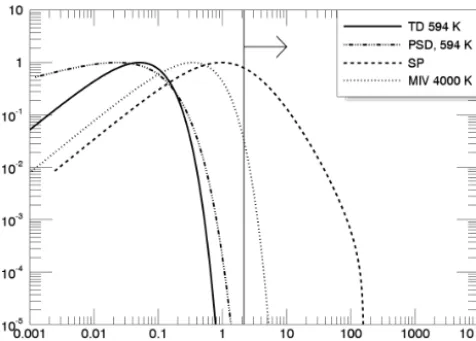
re-Figure 1. Normalized energy distribution functions for several release mechanisms active on Mercury’s surface to produce the sodium exosphere. The vertical solid line marks the value at which sodium atoms have enough energy to escape the gravitational field of Mercury.
lease (see Eq. 3) shown as thedashed–dottedcurve in Fig. 1, which has a characteristic energy of∼0.1 eV; thus particles can reach higher altitudes compared to those released via TD. As can be seen in the plot, the energies are mostly be-low escape. Finally, atoms released via MIV (dotted curve) are modeled by a thermal distribution with temperatures of 4000 K, thus having higher characteristic energy (0.34 eV) compared to the regular TD. MIV contributes to the exo-sphere in a comparable amount like SP (Wurz et al., 2010) if solar wind sputtering is active. Unfortunately, the micro-meteorite influx onto Mercury’s surface is not known very accurately, as discussed above.
3.3 Sodium in and at the surface
Smyth and Marconi (1995) introduced a qualitative descrip-tion of the fate of sodium atoms ejected in Mercury’s envi-ronment using two populations, the “source” and the “am-bient” atoms. A few years later, Morgan and Killen (1997) expanded the description to include the diffusion of sodium from inside the regolith to the surface and the description of the expanding vapor cloud after the impact of micro-meteorites. Here we consider these two populations; the first population is the so-called source atoms, which are atoms chemically bonded in the minerals on the surface and are re-leased by high-energy processes, either by MIV or SP. The source atoms are predominantly ionically bonded to the oxy-gen in a bulk silicate (Madey et al., 1998) with binding en-ergy larger than 0.5 eV.
The released Na atoms may either escape or fall back on the surface and become ambient particles after few impacts on the surface (measured in experiments by Yakshinskiy and Madey, 1999, 2000, 2004). These particles are thermally
ac-Table 1.Parameters for simulation.
Orbital and geographical parameters All processes
Orbital radius (Rorb(au)) 0.458
True anomaly angle (TAA) 202◦a
Solar zenith angle (SZA) 0◦b
Longitude 0◦
Physical parameters
Number of model particles 106
Surface temperature (K) 594
Surface Na atomic fraction 0.0234c
Global meteoritic infall 10.52 t d−1d
UV flux at surfaceφph(m−2s−1) 1.57×10²⁰
d
Radiation acceleration (brad(cm s−2))f 28
aTaken from the Jet Propulsion Laboratory’s (JPL’s) HORIZONS
Ephemeris (https://ssd.jpl.nasa.gov/horizons.cgi, last access: 19 June 2019).
bLatitude=0◦.cIntermediate Composition (Peplowski et al., 2015). dCalculated for the specificR
orb=0.458au and TAA=20◦from the range
given by Müller et al. (2002) which depends on the orbital distance.eFor
PSD.fSmyth and Marconi (1995).
commodated to the local surface temperature and have coun-terparts absorbed in the regolith with a binding energy less than 0.5 eV, according to Hunten et al. (1988). We model this population by low-energy processes such as TD and PSD. An illustration depicting the different release, returning, and loss fluxes is shown and explained in Sect. 5.1.
4 Model implementation
The MC model, as described above, and the Chamberlain model (as described in the Appendix A) are evaluated for the parameters of the MESSENGER observation conditions as listed in Table 1. In this section we describe in detail how we obtained these parameters.
4.1 Simulation parameters and geometry
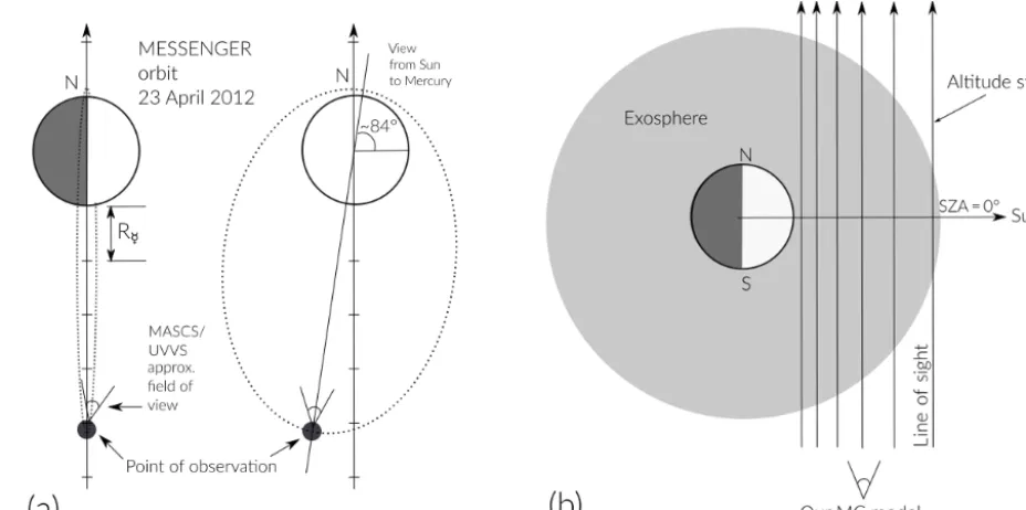
[image:5.612.47.285.66.236.2] [image:5.612.318.535.83.247.2]Figure 2.textbf(a) Representation to scale of MESSENGER’s orbit around Mercury during the time of observations (orbit parameters taken from https://www.nasa.gov).(b)Scheme of the line of sight used in the simulations (distance between altitude steps is not to scale). Solid black lines in(b)represent the altitude steps for integration of the column density when SZA=0◦.
low as 10 km, to several thousand kilometers above the sur-face.
Given the position of the spacecraft with respect to Mer-cury and the direction of the UVVS line of sight during the time of observation, we simulate particles ejected at a latitude of 0◦and a solar zenith angle (SZA) of 0◦and calculated the contribution to the TCD from this position. This is the closest to the real observation geometry that our model can compute. In Fig. 2a we illustrate the orbit geometry and position of the MESSENGER spacecraft during the time of observation. In Fig. 2b we also illustrate the orientation of the tangent (to the surface) altitude steps we used in our model for the inte-gration of the column density. The dawn–dusk asymmetry is not considered because the time of the observation does not include these regions.
The sodium surface atomic fraction, indicated in Table 1, is used to calculate the surface number density and release flux, and it is used only for calculating the source popula-tion produced by the high-energy processes, which are MIV and SP. To simulate the ambient sodium population, which is produced by TD and PSD, we use the surface number density resulting from the returning flux to the surface by MIV and SP.
On the other hand, the radiation pressure depends on the true anomaly angle and the solar zenith angle, and we use the value for radiation acceleration taken from Smyth and Marconi (1995) for the given TAA during the time of obser-vations. We assume the same orbital and physical parameters for our implementation of the Chamberlain model modified by adding radiation pressure.
After computing the density profiles we integrate along the line of sight for different altitude steps and for SZA=0◦to obtain the limb scans as a function of tangent altitude. 4.1.1 Temperature model
According to the infrared measurements made on Mariner 10 (Chase et al., 1976), which only include observations from the nightside up to 08:00 LT on the dayside, and considering Mercury as a blackbody emission radiator, the extrapolated dayside surface temperature as a function of latitudeφ and longitudeθ must follow a “one-fourth” law with an illumi-nation angle and decrease like “1/r2”, whereris the distance of Mercury to the Sun. Neglecting the thermal inertia of Mer-cury’s lithosphere, the local dayside surface temperature for 0<|θ|< π/2 can be written as
Ts(φ, θ )=Tmin+(Tmax−Tmin)(cosφcosθ )1/4,
whereTmaxis the effective temperature at the subsolar point,
Tmin is the nightside temperature, the longitude θ is mea-sured from the planet-Sun axis, and the latitudeφ is mea-sured from the planetary Equator. To determine the effec-tive temperature at the subsolar point we used the blackbody Stefan–Boltzmann law to obtain
Teff≈TSun
" R
Sun
Rorb
21−α
#1/4
, (4)
5778 K is the effective solar temperature, α=0.07 is the albedo (Mallama et al., 2002), and =0.9 is the emissiv-ity (Murcray et al., 1970; Saari and Shorthill, 1972; Hale and Hapke, 2002). During the day of observations Mercury was at a distance ofRorb=0.458 au to the Sun. Using this value and Eq. (4), we calculated a surface temperature of
Teff=TS=594 K at the subsolar point. This is the tempera-ture we used for the TD and PSD calculations.
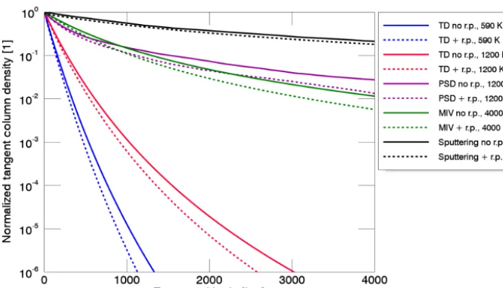
In Fig. 3 we show an example of the tangent column den-sity profiles computed for the different release mechanisms and with different characteristic temperatures. All processes were simulated with and without radiation pressure to com-pare them. We fixed all profiles at altitude zero and a tangent column density normalized to 1 to show the different shapes and slopes for the different mechanisms and different physi-cal parameters specified in the legend.
5 Results and discussion
Using the parameters listed in Table 1, we simulate sodium atoms released via TD, PSD, MIV, and SP and calculated the exospheric density profiles up to 105km. The integral along the line of sight gives us the column density, and if we choose the tangent altitude, we also obtain the TCD as a function of altitude. The surface TCD and released flux obtained from the simulation for each mechanism are listed in Table 2. In-dependently, we also implemented the Chamberlain model in the same fashion as Cassidy et al. (2015) did to compare it to our results (see description in Appendix A).
Figure 4 includes two plots where we show the derived MESSENGER observations (black cross marks) together with the results from our MC simulations and the results us-ing the Chamberlain model. In Fig. 4a, we plot the sodium TCD as a function of altitude for TD (dashed black curve), MIV (dashed grey curves), SP (dashed–dotted grey curve), and PSD (vertical-dash black curve). The results using the Chamberlain model with the modification for radiation pres-sure are also plotted: the curve with square symbols cor-responds to a surface temperature of 594 K, and the curve with circle symbols corresponds to an assumed tempera-ture of 2500 K, with the TCD at the surface of this com-ponent adjusted to match the observations. The sum of the two Chamberlain profiles is represented by the solid light-greycurve. In Fig. 4b, we only plot our MC results for TD withT =594 K, and MIV (multiplied by a factor of 0.5) for
T = [3000,4000,5000]K, together with the derived MES-SENGER observations. We would like to point out again that no fitting to any surface density was applied in our model. Rather, the surface density is a result from the model itself.
At low altitudes the Chamberlain model and the TD sim-ulation for the surface temperature agree very well, and both also agree reasonably well with the observations, which is expected from a Maxwellian population thermalized with the surface. Note that the calculated thermal profiles, both with
the Chamberlain model and with our MC model, are based on the surface temperature, which was derived separately from the orbit position of Mercury, and they were not fitted to the data. The release fluxes for TD and PSD are both calculated from the ambient sodium population atoms, which we de-rived in the next section. The fall-off above 1000 km of the TD 594 K curve is a result of the loss of neutral sodium atoms due to ionization. Compared to any other mechanism mod-eled here, TD is the best match for the observations at low altitudes.
At altitudes above∼600 km the Chamberlain model for 594 K shows densities that are too low, and only a high-temperature component of 2500 K fits the data, similar to Cassidy et al. (2015). The SP curve is too flat and does not match the observations at any given altitude. As described further on, and as shown in Fig. 6, the sputtered component of the tangent column density is expected to be substantial mainly at high latitudes, but the observation geometry gives preference to mechanisms happening at low latitudes, around the subsolar point.
The limitation of Chamberlain theory (Chamberlain, 1963) in this context is that it was originally developed for Earth’s exosphere where the only controlling factors consid-ered are the gravitational attraction and the “thermal energy conducted from below” (also known as exobase). For the case of Mercury, the only layer below the exosphere is the surface. Meaning that, the only source mechanism of exo-spheric particles considered in Chamberlain model is what we consider in our MC model to be thermal desorption.
Using the Chamberlain theory implies that the only way to increase the particles’ characteristic energy (and thus able to reach high altitudes) is by increasing the surface temperature. One way to do this is by micro-meteorite impacts, which can lead to a Maxwellian exospheric population with a tempera-ture of the order of a few thousand kelvins, which can explain the high-energy component in the observations. Another way to increase the temperature is by heating the surface with so-lar radiation. But as calculated, the surface temperature of Mercury at the subsolar point and at TAA=202◦is 594 K. This temperature is not enough to let particles reach high al-titudes; much higher temperatures are needed, as shown in Fig. 4. Consequently, the Chamberlain model works fine only for an exospheric population that is in thermal equilibrium with the surface temperature. For other non-Maxwellian and more energetic populations, the Chamberlain model is inad-equate.
Figure 3.Column density profiles as a function of tangent altitude for Na where the column density at the surface is normalized to 1 and for the different release mechanisms: TD, PSD, MIV, and SP with and without radiation pressure (r.p.) centered at subsolar point and for different surface temperature values. The simulation was done with an ensemble of 106particles and Mercury at TAA=0202◦andRorb=0.458 au.
Figure 4. (a)Plots of the derived TCD from observations (black crosses), of the results from our calculations with no correction factors, and of the results using the Chamberlain model. The resulting TCD profiles from our MC model are plotted as follows: TD is the dashed black curve, MIV between 3000 and 5000 K is the shaded red area, the dashed-grey curve is MIV with a mean temperature of 4000 K, SP is the dashed–dotted grey curve, and PSD is the vertical-dash curve. The resulting profiles using the Chamberlain model are represented as the square- and circle-symbol curves. The sum of the two Chamberlain profiles represented by the solid light-grey curve.(b)Plots of the derived TCD from observations (black crosses) and of the results from our calculations: the dashed black curve is for TD, the results for MIV between 3000 and 5000 K are the shaded red area, the dashed grey curve is MIV with a mean temperature of 4000 K. MIV curves were multiplied by one-half. The sum of TD and MIV profiles is shown as the solid black curve.
is reached by adjusting the surface column density by only a factor of 0.5. Moreover, provided that the high-altitude data above 3000 km shown in Fig. 4 could be removed due to, for instance, stray-light contamination, instrumental effects, or the light coming from a background star, an MIV profile us-ing a temperature between 3000–4000 K would better agree with the data.
[image:8.612.59.538.331.499.2]for precipitating ion fluxes of the cusp region. Since the ob-servations are at the subsolar point, the surface is shielded from precipitating ions (Kallio and Janhunen, 2003), and the SP contribution to the exosphere for these observations has to be considered to be an upper limit as well. Moreover, the TCD from SP falls off much less with altitude than the ob-servations.
5.1 Source and loss fluxes
The sodium loss from the exosphere has to be supplied by Na from the surface to sustain a stable exosphere over several Mercury years as it was observed (Cassidy et al., 2015). As mentioned in Sect. 3.3, the source population of Na to the exosphere is considered to come mainly from the release via SP and MIV. The fraction of this population that comes back to the surface will become the ambient population and be available for TD and PSD. The conservation of mass allows us to quantify the amount of Na in the ambient population at the subsolar point, which is available for TD, by considering that the sum of the Na diffused from regolith to the surface plus the return fluxes from MIV and SP has to be equal the loss due to TD. Mathematically, the latter is expressed as
8Ambientsource =8Diff.+8MIVreturn+8SPreturn, (5)
8Ambientloss =8TDrelease·χTotTD, (6) whereχ is the total fraction of Na loss, which includes the losses by ionization and gravitational escape. 8Diff. is the diffusion-limited exospheric flux calculated by Killen et al. (2004) to be<107cm−2s−1. Note that the fluxes’ subscript source and loss are calculated just for the ambient popula-tion and do not represent the global flux. For a steady-state system,
8Ambientsource −8Ambientloss =0. (7) Combining Eqs. (5), (6), and (7), we derive8TDreleaseas fol-lows:
8TDrelease=8Diff.+8 MIV
return+8SPreturn
χTotTD
=1.0×10
7cm−2s−1+(5.4×10⁵+3.28×10⁵)cm−2s−1 0.0102
=1.06×109cm−2s−1. (8) From Eq. (8) we can derive the surface density as
n0= 8TDrelease
vth =1.44×10
10m−3, wherev the=
√
8kBT /π m= 739 m s−1. The radial column density, NC, can be approximated as NC≈n0·H=8.21×10¹⁴m−2=8.21× 1010cm−2. The rest of the results of our simulations, together with the derived quantities for the ambient population, are shown in Table 2.
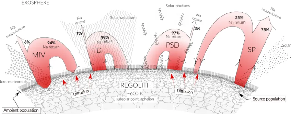
Figure 5 is a scheme illustrating the Na release processes and fate due to the different release mechanisms. For the
given observations, we calculated the Na release flux from the surface and determined the losses for each process. The fraction of Na that is not lost returns to the surface and be-comes part of the ambient population available for TD and PSD.
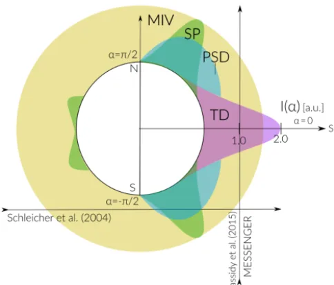
Figure 6 is an illustration of the spatial distribution of the derived released Na fluxes as a function of solar zenith angle. The radial scale represents the magnitude difference of the release flux “intensity”,I (α), for the different release mech-anisms (the units are arbitrary). Note that this diagram does not represent the spatial distribution of Na depending on the mechanism but just the magnitude of the release flux for each mechanism. At the subsolar point, the main contribution of Na to the exosphere is TD, with a release flux of 2 orders of magnitude higher compared to the other release processes and with an exponential decay towards the poles because of the strong temperature dependence of sublimation. The solar wind sputtering on the surface acts mainly at high latitudes (α≈ ±π/2) and is also a strong function of latitude decay. We consider that MIV acts uniformly on the entire planet, thus the release flux is not angle dependent. PSD has a co-sine dependence with SZA, but since it competes with TD it is most important at mid-latitudes to high latitudes.
This illustration shows the main release mechanisms given a certain line-of-sight observation geometry. For instance, the ground-based observations done by Schleicher et al. (2004) during Mercury’s transit had a limb line of sight similar to the horizontal line shown in Fig. 6. The main contribution for those limb observations whenα≈ ±π/2 includes a sum of SP and PSD, which provides a sputter high-energy Na ex-osphere and a low-energy photo-desorbed ambient Na pop-ulation, which was already discussed by Mura et al. (2009). On the other hand, the vertical line of sight path crossing TD and MIV represents the line of sight of the approximate di-rection of MESSENGER’s field of view during observations on 23 April 2012 (Cassidy et al., 2015) and discussed here. If observations are made with a line of sight corresponding toα≈ ±π/4 for instance, the analysis of the source mecha-nisms becomes complicated because all release mechamecha-nisms will be active in some extent, and thus it will be difficult to differentiate them.
Table 2.Results from the MC simulation.
Property TD MIV PSD SP
Scale height (km) 57 431 232 748
Surface density (n0(m−3))a 1.44×10¹⁰ 5.97×10⁶ 3.45×10¹⁰ 3.72×10⁶
Column density (NC (cm−2)) 8.21×10¹⁰ 2.57×10⁸ 8.0×10¹¹ 2.79×10⁸ Total released Na flux (cm−2s−1) 1.06×10⁹ 5.74×10⁵ 3.63×10⁹b 1.32×10⁶
Total fraction of lost particlesc 0.0102 0.0589 0.0307 0.7510
aBased on Na surface fraction from intermediate composition (Peplowski et al., 2015) and used for MIV, PSD, and SP. bAdjusted to observations by a multiplication factor of 4×10⁻⁴and considered an upper limit.cIncluding the losses by
[image:10.612.64.539.216.402.2]gravitational escape and ionization.
Figure 5.Scheme illustrating the different released fluxes of Na due to the different release mechanisms from the mineral compound (the source population) and from surface (the ambient population). The illustration is not to scale.
above the surface and the evaporated flux by using the em-pirical equation for the Na vapor pressure (Lide, 2003), and considering a surface temperature ofT =594 K at the subso-lar point, this gives a sodium vapor pressure ofP0=7.44 Pa. The corresponding theoretical evaporated flux of sodium atoms from this surface reservoir would be 6.71× 10²¹atoms cm−2s−1. This value is 14 orders of magnitude higher than the thermal Na release flux we derived from mea-surements, which is 4.34×10⁸atoms cm−2s−1. Even if the atomic Na is bound to the surface with a higher binding en-ergy, the sublimation flux will still be enormous at this tem-perature. Thus, it is clear that the TD flux is limited by the availability of ambient Na on the surface, and given the large difference in theoretical and derived release fluxes, all the ambient Na is in the exosphere and not on the surface near the subsolar point. This implies that all the ambient sodium released from the bulk or that has fallen back onto the surface near the subsolar point will be immediately evaporated to the exosphere, leaving no atomic Na left in areas near the subso-lar point. Therefore, based on these considerations, PSD can not compete to desorb sodium because there is no Na left available on the surface.
Figure 6.Scheme of the intensity distributions for the different re-lease mechanisms as a function of solar zenith angle. The units are arbitrary, but orders of magnitude are taken from the results of our model. The horizontal arrow is an example of the line of sight of the ground-based observations by Schleicher et al. (2004). Vertical arrow represents the approximate direction of MESSENGER’s field of view during observations on 23 April 2012 (Cassidy et al., 2015).
6 Conclusions
We present the results of our Monte Carlo model of the Her-mean sodium exosphere and compare them with the sodium tangent column density profile derived from MASCS/UVVS measurements during the day on 23 April 2012 (Cassidy et al., 2015). Using the correct parameters for TAA andTSfor the day of the observations, we calculate the density profiles of sodium atoms ejected from Mercury’s surface through TD, PSD, MIV, and SP as release mechanisms.
We reproduce the derived sodium TCD profile as a func-tion of altitude: below 500 km, the dominant release mecha-nism of Na is TD with a surface temperature of 594 K, cor-responding to a characteristic energy of 0.06 eV. Because of the very high release fluxes, the Na in the exosphere near the surface is due to TD, limited by the supply of available Na atoms on the surface. Only at higher altitudes does the con-tribution by MIV prevail up to the observed 4000 km with a characteristic energy of 0.34 eV.
For the first 500 km with the MC model TD results agree well with the Chamberlain model using a local surface tem-perature of 594 K, and both agree with the measurements. As we go farther away from Mercury’s surface, though, there is a more energetic component of Na atoms in the exosphere, which we find to be the result of MIV.
We have also shown that if there would be an ambient sodium layer available on the surface at the subsolar point, this would have to be immediately evaporated due to the
high volatility of Na at such a high surface temperature at the given observation time. The Na release by TD is strongly limited by the supply of free Na to the surface at the local sur-face temperature. Moreover, release by PSD can only be re-sponsible for the Na exosphere population at higher altitudes because of the higher energies of the released Na atoms. However, we find that we can only give an upper limit for the release of Na via PSD for the investigated observations.
Our results diverge substantially from the results by Cas-sidy et al. (2015). While their work is explanatory and sug-gests the derived observations in terms of two thermal release populations using the Chamberlain model, it seems like they arrive at a confounding near-to-the-surface sodium tempera-ture of 1200 K. Using their assumptions and the Chamberlain model we get good agreement of our model (MC and Cham-berlain) for the calculated surface temperature, which is half their value, and the results using our MC model confirm the same number.
As mentioned before, our results apply to the specific ob-servation conditions we discussed. As shown in our diagram in Fig. 6, for other observation geometries, i.e., a different line of sight and TAA, other surface release mechanisms might be active and can dominate over others. Future work will include a larger data set with different observation con-ditions to test our model and determine the influence of other release processes.
The use of mass spectrometers is crucial for studying the surface composition of Mercury and ultimately understand-ing the origin of species found in the exosphere, since they come from the regolith and crust (except for the noble gases, hydrogen, and a few volatile species such as sulfur, which are abundant in the micro-meteorite population). To prepare for the SERENA investigation (Orsini et al., 2010), to be performed aboard the ESA’s BepiColombo planetary orbiter (Milillo et al., 2010), we have updated and extended our MC model, originally developed by Wurz and Lammer (2003), which is a tool to quantitatively predict exospheric densities for several release processes using the actual physical param-eters of the release process.
Appendix A: Chamberlain model implementation Chamberlain’s model (Chamberlain, 1963) is based on Li-ouville’s theorem applied to a collisionless exosphere where the gravitational attraction and the thermal energy conducted from below are the controlling factors. The Liouville equa-tion is solved using a Maxwellian distribuequa-tion as the bound-ary condition at the exobase. The velocity distribution is then integrated in the region allowed by the trajectory in a gravita-tional field and over the velocity space, which can be divided into different populations that represent different types of particle orbits:ballistic(captive particles whose orbits inter-sect the critical level, i.e., surface in Mercury’s case), satel-lite (captive particles orbiting above the critical level), and
escaping(particle’s velocity is larger than the escape veloc-ity). This leads to analytic expressions for the density dis-tributions and the loss flux. The number density at a given altituderis given by
n(r)=n(rc)exp [−(λc−λ)]ζ (λ), (A1) where the parameter λrepresents the absolute value of the potential energy expressed in units ofkBTcas follows:
λc(r)=
GMm kBTcr
=v 2 esc
V2, (A2)
where vesc=(2GM/rc)1/2 is the escape velocity andV =
(2kBTc/m)
1/2 is the most probable Maxwellian velocity (thermal velocity),Gis the gravitational constant,Mis the mass of the planet,mis the mass of the species,kBthe Boltz-mann constant, Tc is the exobase temperature, andr is the radial distance from the center of the planet. The subscript “c” stands for critical level that corresponds to the exobase, which corresponds to Mercury’s surface in this case.
Equation (A1) is a combination of the barometric den-sity equation with a partition function ζ (λ), where n(rc)is the density at the critical level. The factor ζ may be re-garded as the fraction of the isotropic Maxwellian distribu-tion that is present at a given altitude, subject to conserva-tion of energy and angular momentum. For no dynamical restrictions to the orbit, ζ=1, which leads to the general-ized form of the (isothermal) barometric law. However, at substantial distances above the critical level the barometric law breaks down because the pressure at large distances is decidedly directional and the mean kinetic energy per atom decreases. The atmosphere is not strictly in hydrostatic equi-librium, moreover it is expanding slightly; i.e., some matter is being lost, which in the kinetic theory corresponds to evap-orative loss. To treat the density distribution accurately it is necessary to examine the individual particle orbits, which is the case whenζ 6=0. The analytical expressions ofζfor each class of particle orbits can be found in Chamberlain (1963). The effect of radiation pressure on sodium atoms was also incorporated following Bishop and Chamberlain (1989). Ex-amples of sodium column density profiles for the different
types of trajectories are displayed in Fig. A1, considering a surface temperature ofTc=594 K.
On the other hand, sodium atoms in the atmosphere of Mercury can be accelerated by solar radiation pressure re-sulting from resonant scattering of solar photons. In earlier works was suggested that radiation pressure could sweep sodium off the planet, provided that the sodium is non-thermal (e.g., Ip, 1986; Bishop and Chamberlain, 1989; Wang and Ip, 2011). Under the influence of radiation pres-sure, particles’ trajectories can depart significantly from Ke-plerian counterparts, thus modifying the exosphere structure. As a consequence, the sodium atoms might be expected to be pushed away from the Sun towards the nightside of Mercury as the radiation pressure increases. It has been shown that for sodium atoms, radiation acceleration can be up to 54 % of the surface gravity (Smyth and Marconi, 1995). We follow Bishop and Chamberlain (1989) by modifying the potential energy function, |λ(r)|, and we implement the solar radia-tion acceleraradia-tion expression as used by Wang and Ip (2011). Equation (A3) is the new expression for the potential energy in units ofkBTand is a combination of the acceleration by gravity and radiation forces:
λ(r)=GMm
kBTr
−mbrprcos(θ )
kBT
, (A3)
Figure A1.Examples of the TCD profiles for sodium for an exobase temperature of 594 K using the Chamberlain model. The pink curve represents the density profile for the barometric law; the green curve represents a combination of ballistic, satellite, and escape orbits; and the blue curve represents density profiles including ballistic and escaping particles.
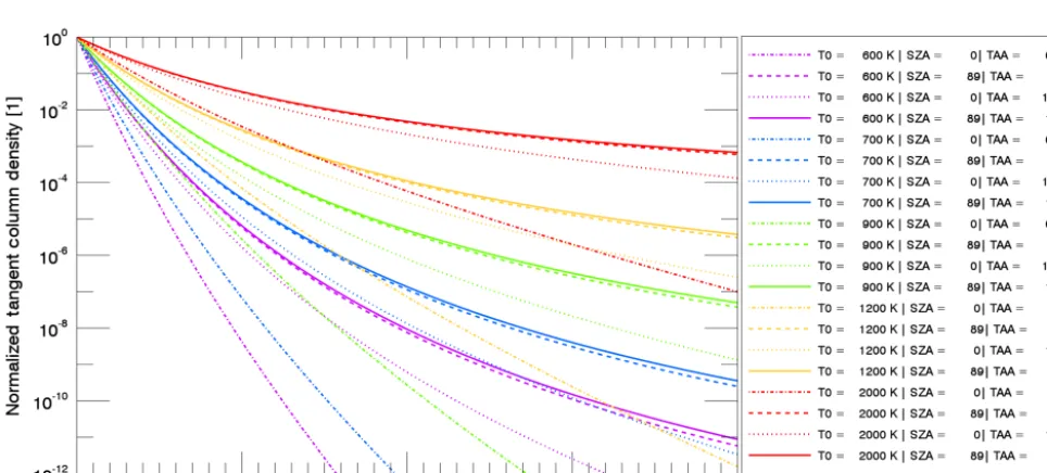
Figure A2.Examples of the TCD profiles for sodium using Chamberlain model for different values of temperature,T0=[600, 700, 900,
[image:13.612.56.538.427.645.2]Author contributions. PW conceived the presented idea and super-vised the project. The writing of the original draft was done by DG, and the review and editing were done by PW and AV. Validation of results was done by AV and PW. Illustrations were done by DG. All the authors developed the theory and performed the computations. All authors discussed the results and contributed to the final paper.
Competing interests. The authors declare that they have no conflict of interest.
Acknowledgements. The first author also wants to thank An-dré Galli for his support and help while writing this paper. We also thank the Linux Cluster UBELIX team for letting us use their clus-ter to run our simulations. We also want to thank Willi Exner for validating some of our calculations.
Financial support. This research has been supported by the Swiss National Science Foundation (grant no. 200020_172488).
Review statement. This paper was edited by Stephanie C. Werner and reviewed by Rosemary Killen and Anna Milillo.
References
Anderson, B. J., Johnson, C. L., Korth, H., Purucker, M. E., Winslow, R. M., Slavin, J. A., Solomon, S. C., McNutt Jr., R. L., Raines, J. M., and Zurbuchen, T. H.: The global magnetic field of Mercury from MESSENGER orbital observations, Science, 333, 1859–1862, https://doi.org/10.1126/science.1211001, 2011. Bishop, J. and Chamberlain, J. W.: Radiation pressure dynamics in
planetary exospheres: A “natural” framework, Icarus, 81, 145– 163, https://doi.org/10.1016/0019-1035(89)90131-0, 1989. Borin, P., Cremonese, G., Marzari, F., Bruno, M., and Marchi,
S.: Statistical analysis of micrometeorites flux on Mercury, As-tron. Astrophys., 503, 259–264, https://doi.org/10.1051/0004-6361/200912080, 2009.
Borin, P., Bruno, M., Cremonese, G., and Marzari, F.: Estimate of the neutral atoms’ contribution to the Mercury exosphere caused by a new flux of micrometeoroids, Astron. Astrophys., 517, A89, https://doi.org/10.1051/0004-6361/201014312, 2010.
Broadfoot, A. L., Shemansky, D. E., and Kumar, S.: Mariner 10 – Mercury atmosphere, Geophys. Res. Lett., 3, 577–580. https://doi.org/10.1029/GL003i010p00577, 1976.
Burger, M. H., Killen, R. M., Vervack Jr., R. J., Bradley, E. T., McClintock, W. E., Sarantos, M., Benna, M., and Mouawad, N.: Monte Carlo modeling of sodium in Mercury’s exosphere during the first two MESSENGER flybys, Icarus, 209, 63–74, https://doi.org/10.1016/j.icarus.2010.05.007, 2010.
Cassidy, T. A., Merkel, A. W., Burger, M. H., Sarantos, M., Killen, R. M., McClintock, W. E., and Vervack, R. J.: Mercury’s seasonal sodium exosphere: MESSENGER orbital observations, Icarus, 248, 547–559, https://doi.org/10.1016/j.icarus.2014.10.037, 2015.
Cassidy, T. A., McClintock, W. E., Killen, R. M., Saran-tos, M., Merkel, A. W., Vervack, R. J., Burger, and
Matthew, H.: A cold-pole enhancement in Mercury’s
sodium exosphere, Geophys. Res. Lett., 43, 11121–11128, https://doi.org/10.1002/2016GL071071, 2016.
Chamberlain, J. W.: Planetary coronae and
atmo-spheric evaporation, Planet. Space Sci., 11, 901–960,
https://doi.org/10.1016/0032-0633(63)90122-3, 1963.
Chase, S. C., Jr., Miner, E. D., Morrison, D., Muench, G., and Neugebauer, G.: Mariner 10 infrared radiometer results – Temperatures and thermal properties of the surface of Mercury, Icarus, 28, 565–578, https://doi.org/10.1016/0019-1035(76)90130-5, 1976.
Cintala, M. J.: Impact-induced thermal effects in the lunar and Mercurian regoliths, J. Geophys. Res., 97, 947–973, https://doi.org/10.1029/91JE02207, 1992.
Collier, M. R., Moore, T. E., Ogilvie, K. W., Chornay, D. J., Keller, M. C., Fuselier, B. L., Quinn, J., Wurz, P., Wuest, P., and Hsieh, K. C.: Dust in the wind: The dust geometric cross section at 1 AU based on neutral solar wind observa-tions, Solar Wind X, American Institute Physics, 679, 790–793, https://doi.org/10.1063/1.161871, 2003.
Eichhorn, G.: Heating and vaporization during
hyperve-locity particle impact, Planet. Space Sci., 26, 463–467, https://doi.org/10.1016/0032-0633(78)90067-3, 1978a.
Gamborino, D. and Wurz, P.: Velocity distribution of Na released by photons from planetary surfaces, Planet. Space Sci., 159, 97– 104, https://doi.org/10.1016/j.pss.2018.04.021, 2018.
Hale, A. S. and Hapke, B.: A Time-Dependent Model of Radia-tive and ConducRadia-tive Thermal Energy Transport in Planetary Re-goliths with Applications to the Moon and Mercury, Icarus, 156, 318–334, https://doi.org/10.1006/icar.2001.6768, 2002. Hunten, D. M., Shemansky, D. E., and Morgan, T. H.: The
Mer-cury atmosphere, in: MerMer-cury, edited by: Vilas, F., Chapman, C. R., and Matthews, M. S., University of Arizona Press, 562–612, 1988.
Ip, W. H.: The sodium exosphere and magnetosphere
of Mercury, Geophys. Res. Lett., 13, 423–426,
https://doi.org/10.1029/GL013i005p00423, 1986.
Johnson, R. E., Leblanc, F., Yakshinskiy, B. V., and Madey, T. E.: Energy distributions for desorption of sodium and potas-sium from ice: the Na/K ratio at Europa, Icarus, 156, 136–142, https://doi.org/10.1006/icar.2001.6763, 2002.
Kallio, E. and Janhunen, P.: Solar wind and magnetospheric ion impact on Mercury’s surface, Geophys. Res. Lett., 30, 1877, https://doi.org/10.1029/2003GL017842, 2003.
Killen, R. M., Potter, A. E., and Morgan, T. H.: Spatial distribution of sodium vapor in the atmosphere of Mercury, Icarus, 85, 145– 167, https://doi.org/10.1016/0019-1035(90)90108-L, 1990. Killen, R. M., Potter, A., Fitzsimmons, A., and Morgan, T. H.:
Sodium D2 line profiles: clues to the temperature structure of Mercury’s exosphere, Planet. Space Sci., 47, 1449–1458, https://doi.org/10.1016/S0032-0633(99)00071-9, 1999. Killen, R., G. Sarantos, M., Potter, A. E., and Reiff, P.: Source rates
and ion recycling rates for Na and K in Mercury’s atmosphere, Icarus, 171, 1–19, https://doi.org/10.1016/j.icarus.2004.04.007, 2007.
M., Milillo, A., and Mura, A.: Processes that promote and de-plete the exosphere of Mercury, Space Sci. Rev., 132, 433–509, https://doi.org/10.1007/s11214-007-9232-0, 2007.
Killen R., Shemansky, D., and Mouawad N.: Expected emission from Mercury’s exospheric species, and their
ultraviolet-visible signatures, Astrophys. J. Suppl., 181, 351–359,
https://doi.org/10.1088/0067-0049/181/2/351, 2009.
Leblanc, F., Delcourt, D., and Johnson, R. E.: Mercury’s sodium exosphere: magnetospheric ion recycling, J. Geophys. Res., 108, 5136, https://doi.org/10.1029/2003JE002151, 2003.
Leblanc, F. Doressoundiram, A., Schneider, N., Massetti, S., Wed-lund, M., López, Ariste, A., Barbieri, C., Mangano, V., and Cre-monese, G.: Short-term variations of Mercury’s Na exosphere observed with very high spectral resolution, Geophys. Res. Lett., 36, L07201, https://doi.org/10.1029/2009GL038089, 2009. Leblanc, F. and Johnson, R. E.: Mercury exosphere I. Global
cir-culation model of its sodium component, Icarus, 209, 280–300, https://doi.org/10.1016/j.icarus.2010.04.020, 2010.
Lide, D. R.: CRC Handbook of Chemistry and Physics, 84th Edi-tion. CRC Press. Boca Raton, Florida, Section 4, 2003. Madey, Theodore E., Yakshinskiy, B. V., Ageev, V. N., and
John-son, R. E.: Desorption of alkali atoms and ions from oxide surfaces – Relevance to origins of Na and K in atmospheres of Mercury and the Moon, J. Geophys. Res., 103, 5873–5887, https://doi.org/10.1029/98JE00230, 1998.
Mallama, A., Wang, D., and Howard, R. A.:
Photome-try of Mercury from SOHO/LASCO and Earth: The
Phase Function from 2◦ to 170◦, Icarus, 155, 253–264,
https://doi.org/10.1006/icar.2001.6723, 2002.
Mangano, V., Massetti, S., Milillo, A., Plainaki, C., Orsini, S., Rispoli, R., and Leblanc, F.: THEMIS Na exosphere observations of Mercury and their correlation with in-situ magnetic field mea-surements by MESSENGER, Planet. Space Sci., 115, 102–109, https://doi.org/10.1016/j.pss.2015.04.001, 2015.
Massetti, S., Orsini, S., Milillo, A., Mura, A., DeAngelis, E., Lammer, H., and Wurz, P.: Mapping of the cusp plasma pre-cipitation on the surface of Mercury, Icarus, 166, 229–237, https://doi.org/10.1016/j.icarus.2003.08.005, 2003.
Massetti, S., Mangano, V., Milillo, A., Mura, A., Orsini, S., Plainaki, C.: Short-term observations of double-peaked Na emis-sion from Mercury’s exosphere, Geophys. Res. Lett., 44, 2970– 2977, https://doi.org/10.1002/2017GL073090, 2017.
McClintock, W. E., Bradley, E. T., Vervack, R. J., Killen, R. M., Sprague, A. L., Izenberg, N. R., and Solomon, S. C.: Mercury’s Exosphere: Observations During
MES-SENGER’s First Mercury Flyby, Science, 321, 92–94,
https://doi.org/10.1126/science.1159467, 2008.
McGrath, M. A., Johnson, R. E., and Lanzerotti, L. J.: Sputter-ing of sodium on the planet Mercury, Nature, 323, 694–696, https://doi.org/10.1038/323694a0, 1986.
Milillo, A., Fujimoto, M., Kallio, E., Kameda, S., Leblanc, F., Narita, Y., Cremonese, G., Laakso, H., Laurenza, M., Mas-setti, S., McKenna-Lawlor, S., Mura, A., Nakamura, R., Omura, Y., Rothery, D. A., Seki, K., Storini, M., Wurz, P., Baumjo-hann, W., Bunce, E., Kasaba, Y., Helbert, J., and Sprague, A.: The BepiColombo mission: an outstanding tool for investigat-ing the Hermean environment, Planet. Space Sci., 58, 40–60, https://doi.org/10.1016/j.pss.2008.06.005, 2010.
Morgan, T. H. and Killen, R. M: A non-stoichiometric model of the composition of the atmospheres of Mercury and the Moon, Planet. Space Sci., 45, 81–94, https://doi.org/10.1016/S0032-0633(96)00099-2, 1997.
Mouawad, N., Burger, M. H., Killen, R. M., Potter, A. E., Mc-Clintock, W. E., Vervack, R. J., Bradley, E. T., Benna, M., and Naidu, S.: Constraints on Mercury’s Na exosphere: Com-bined MESSENGER and ground-based data, Icarus, 211, 21–36, https://doi.org/10.1016/j.icarus.2010.10.019, 2011.
Müller, M., Green, S. F., McBride, N., Koschny, D., Zar-necki, J. C., and Bentley, M. S.: Estimation of the dust flux near Mercury, Planet. Space Sci., 50, 1101–1115, https://doi.org/10.1016/S0032-0633(02)00048-X, 2002. Mura, A., Wurz, P., Lichtenegger, H. I. M., Schleicher, H.,
Lammer, H., Delcourt, D., Milillo, A., Orsini, S., Mas-setti, S., and Khodachenko, M. L.: The sodium exo-sphere of Mercury: Comparison between observations dur-ing Mercury’s transit and model results, Icarus, 200, 1–11. https://doi.org/10.1016/j.icarus.2008.11.014, 2009.
Murcray, F. H., Murcray, D. G., and Williamns, W. J.: In-frared emissivity of lunar surface features, I.
Balloon-borne observations, J. Geophys. Res., 75, 2662–2669,
https://doi.org/10.1029/JB075i014p02662, 1970.
Orsini, S., Livi, S., Torkar, K., Barabash, S., Milillo, A., Wurz, P., Di Lellis, A. M., Kallio, E., and The SERENA team: SER-ENA: A suite of four instruments (ELENA, STROFIO, PICAM, and MIPA) on board BepiColombo-MPO for particle detection in the Hermean evironment, Planet. Space Sci., 58, 166—181, https://doi.org/10.1016/j.pss.2008.09.012, 2010.
Peplowski, P., Lawrence, D., Feldman, W., Goldsten, J., Bazell, D., Evans, L., Head, J., Nittler, L., Solomon, S., and Weider, S.: Geo-chemical terranes of Mercury’s northern hemisphere as revealed by MESSENGER neutron measurements, Icarus, 253, 346–363, https://doi.org/10.1016/j.icarus.2015.02.002, 2015.
Potter, A. E. and Morgan, T. H.: Discovery of sodium in the atmosphere of Mercury, Science, 229, 651–653, https://doi.org/10.1126/science.229.4714.651, 1985.
Potter, A. E. and Morgan, T. H.: Variation of sodium on Mercury with solar radiation pressure, Icarus, 71, 472–477, https://doi.org/10.1016/0019-1035(87)90041-8, 1987.
Potter, A. E. and Morgan, T. H.: Sodium and potassium atmospheres of Mercury, Planet. Space Sci., 45, 95–100, https://doi.org/10.1016/S0032-0633(96)00100-6, 1997. Potter, A. E., Killen, R. M., and Morgan, T. H.: The sodium
tail of Mercury, Meteorit. Planet. Sci., 37, 1165–1172, https://doi.org/10.1111/j.1945-5100.2002.tb00886.x, 2002. Potter, A. E., Killen, R. M., and Sarantos, M.: Spatial
distribution of sodium on Mercury, Icarus, 181, 1–12, https://doi.org/10.1016/j.icarus.2005.10.026, 2006.
Potter, A. E., Killen, R. M., and Morgan, T. H.: Solar radiation ac-celeration effects on Mercury sodium emission, Icarus, 186, 571– 580, https://doi.org/10.1016/j.icarus.2006.09.025, 2007. Raines, J. M., Gershman, D. J., Slavin, J. A., Zurbuchen, T. H.,
Saari, J. M. and Shorthill, R. W.: The sunlit lunar surface. I. Albedo studies and full Moon temperature distribution, The Moon, 5, 161–178, https://doi.org/10.1007/BF00562111, 1972.
Sarantos, M., Slavin, J. A., Benna, M., Boardsen, S. A., Killen, R. M., Schriver, D., and Travnicek, P.: Sodium-ion pickup observed above the magnetopause during MESSENGER’s first Mercury flyby: Constraints on neutral exospheric models, Geophys. Res. Lett., 36, L04106, https://doi.org/10.1029/2008GL036207, 2009. Schleicher, H., Wiedemann, G., Wohl, H., Berkefeld, T., and Soltau, D.: Detection of neutral sodium above Mercury during the transit on 2003 May 7, Astron. Astrophys., 425, 1119–1124, https://doi.org/10.1051/0004-6361:200 40477, 2004.
Schmidt, C. A.: Monte Carlo modeling of north-south asymmetries in Mercury’s sodium exosphere, J. Geophys. Res.-Space, 118, 4564–4571, https://doi.org/10.1002/jgra.50396, 2013.
Simpson, W. C., Wang, W. K., Yarmo, J. A., and Orlando, T. M.:Photon- and electron-stimulated desorption of O+from zir-conia, Surf. Sci., 423, 225–231, https://doi.org/10.1016/S0039-6028(98)00908-X, 1999.
Smyth, W. H.: Nature and variability of Mercury’s sodium atmo-sphere, Nature, 323, 696–699, https://doi.org/10.1038/323696a0, 1986.
Smyth, W. H. and Marconi, M. L.: Theoretical overview and mod-eling of the sodium and potassium atmosphere of Mercury, As-trophys. J., 441, 839–864, https://doi.org/10.1086/175407, 1995. Sprague, A. L., Schmitt, W. J., and Hill, R. E.:
Mer-cury: Sodium atmospheric enhancements, radar-bright
spots, and visible surface features, Icarus, 136, 60–68, https://doi.org/10.1006/icar.1998.6009, 1998.
Takakuwa, Y., Niwano, M., Nogawa, M., Katakura, H., Matsuyoshi, S., Ishida, H., Kato, H., and Miyamoto, M.: Photon-stimulated desorption of H+ions from oxidized Si(111) surfaces, Japn. J. Appl. Phys., 28, 2581 pp., https://doi.org/10.1143/JJAP.28.2581, 1989.
Vervack, R. J., Killen, R. M., McClintock, W. E., Merkel, A. W., Burger, M. H., Cassidy, T. A., and Sarantos, M.: New discoveries from MESSENGER and insights into Mer-cury’s exosphere, Geophys. Res. Lett., 43, 11545–11551, https://doi.org/10.1002/2016GL071284, 2016.
Vorburger, A., Wurz, P., Lammer, H., Barabash, S., and Mousis, O.: Monte-Carlo simulation of Callisto’s exosphere, Icarus, 262, 14– 29, 2015.
Wang, Y. C. and Ip, W. H.: Source dependency of
ex-ospheric sodium on Mercury, Icarus, 216, 387–402,
https://doi.org/10.1016/j.icarus.2011.09.023, 2011.
Winslow, R. M., Johnson, C. L., Anderson, B. J., Korth, H., Slavin, J. A., Purucker, M. E., and Solomon, S. C.: Ob-servations of Mercury’s northern cusp region with MES-SENGER’s Magnetometer, Geophys. Res. Lett., 39, L08112, https://doi.org/10.1029/2012GL051472, 2012.
Woodruff, D. P., Traum, M. M., Farrell, H. H., Smith, N. V., Johnson, P. D., King, D. A., Benbow, R. L., and Hurych, Z.: Photon- and electron-stimulated desorp-tion from a metal surface, Phys. Rev. B, 21, 5642–5645, https://doi.org/10.1103/PhysRevB.21.5642, 1980.
Wurz, P. and Lammer, H.: Monte-Carlo Simulation of Mercury’s Exosphere, Icarus, 164, 1–13, https://doi.org/10.1016/S0019-1035(03)00123-4, 2003.
Wurz, P., Rohner U., Whitby, J. A., Kolb, C., Lammer, H., Dobnikar P., and Martín-Fernández, J. A.: The Lunar Ex-osphere: The Sputtering Contribution, Icarus, 191, 486–496, https://doi.org/10.1016/j.icarus.2007.04.034, 2007.
Wurz, P., Whitby, J. A., Rohner U., Martín-Fernández, J. A., Lammer, H., and Kolb, C.: Self-consistent modeling of Mer-cury’s exosphere by sputtering, micro-meteorite impact and photon-stimulated desorption, Planet Space Sci., 58 1599–1616, https://doi.org/10.1016/j.pss.2010.08.003, 2010.
Yakshinskiy, B. V. and Madey, T. E.: Photon-stimulated desorption as a substantial source of sodium in the lunar atmosphere, Nature, 400, 642–644, https://doi.org/10.1038/23204, 1999.
Yakshinskiy, B. V. and Madey, T. E.: Desorption induced by electronic transitions of Na from SiO2: relevance to
tenuous planetary atmospheres, Surf. Sci., 451, 160–165, https://doi.org/10.1016/S0039-6028(00)00022-4, 2000. Yakshinskiy, B. V. and Madey, T. E.: Photon-stimulated
desorp-tion of Na from a lunar sample: temperature-dependent effects, Icarus, 168, 53–59, https://doi.org/10.1016/j.icarus.2003.12.007, 2004.
Yakshinskiy, B. V. and Madey, T. E.:
Temperature-dependent DIET of alkalis from SiO2 films:
Compar-ison with a lunar sample, Surf. Sci., 593, 202–209,
https://doi.org/10.1016/j.susc.2005.06.062, 2005.