https://doi.org/10.5194/angeo-36-1117-2018 © Author(s) 2018. This work is distributed under the Creative Commons Attribution 4.0 License.
Data mining for vortices on the Earth’s magnetosphere –
algorithm application for detection and analysis
Yaireska M. Collado-Vega1, Virginia L. Kalb2, David G. Sibeck1, Kyoung-Joo Hwang3, and Lutz Rastätter1 1NASA Goddard Space Flight Center, Space Weather Laboratory, Code 674, Greenbelt, MD, USA
2NASA Goddard Space Flight Center, Terrestrial Information Systems, Code 619, Greenbelt, MD, USA 3Southwest Research Institute, San Antonio, TX, USA
Correspondence:Yaireska M. Collado-Vega ([email protected])
Received: 4 December 2017 – Revised: 11 June 2018 – Accepted: 13 June 2018 – Published: 16 August 2018
Abstract. Unsteady processes in the solar wind– magnetosphere interaction, such as vortices developed at the magnetopause boundary by the Kelvin–Helmholtz instability, may contribute to the process of mass, momen-tum and energy transfer into the Earth’s magnetosphere. The research described in this paper validates an algorithm to automatically detect and characterize vortices based on velocity data from simulations. The vortex identification algorithm (VIA) systematically searches the 3-D velocity fields to identify critical points where the magnitude of the velocity vector vanishes. The velocity gradient tensor is computed and its invariants are used to assess vortex struc-ture in the flow field. We use the Community Coordinated Modeling Center (CCMC) Runs on Request capability to create a series of model runs initialized from the conditions observed by the Cluster mission in the Hwang et al. (2011) analysis of Kelvin–Helmholtz vortices observed during southward interplanetary magnetic field (IMF) conditions. We analyze further the properties of the vortices found in the runs, including the velocity changes within their motion across the magnetosheath. We also demonstrate the potential of our tool to identify and characterize other transient fea-tures (e.g., flux transfer events, FTEs) with vortical internal structures. We find that the vortices are associated with flows on the magnetosheath side of the magnetopause that reach speeds greater than the solar wind speed at the bow shock. Keywords. Magnetospheric physics (MHD waves and in-stabilities; solar wind–magnetosphere interactions) – space plasma physics (numerical simulation studies)
1 Introduction
Large eddy structures or vortices can mark regions of intense flow activity and are important in understanding physical transport processes. Coherent vortical structures are often the most important physical mechanisms for generating and sus-taining turbulent motion. One important mechanism of vor-tex generation is the Kelvin–Helmholtz instability. When the different layers of a stratified fluid are in relative motion, the shear causes a wrinkling of their interface, which is amplified by nonlinearities to produce vortical motion. Such a situation exists when the solar wind passes the Earth’s magnetopause. Finding and studying these vortices is important for under-standing the Sun–Earth connection. Even in the initial stages, these vortices can transfer momentum, energy and mass from the solar wind to the Earth’s magnetosphere (Miura, 1984; Nykyri and Otto, 2001; Hasegawa et al., 2004a).
prefer-1118 Y. M. Collado-Vega et al.: Data mining for vortices
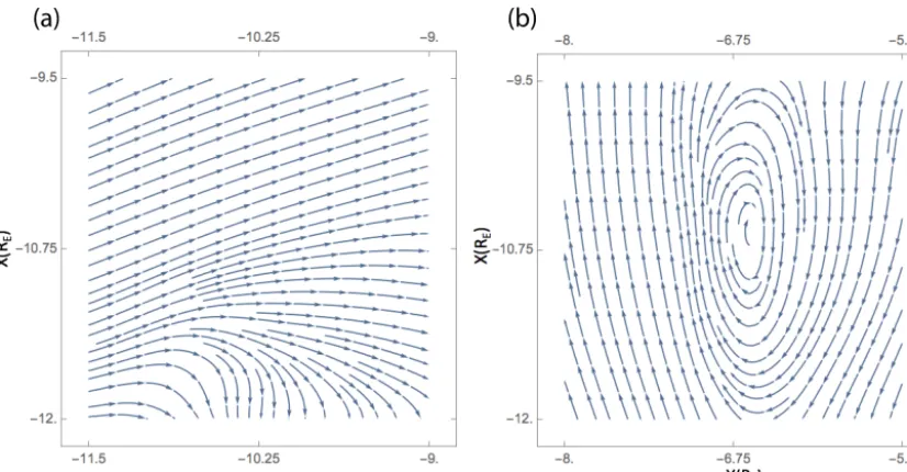
[image:2.612.95.508.70.285.2](a)
(b)
Figure 1.Streamlines are mapped to show an example of the method used to identify vortices in the data. If the norm ofRis greater than the norm ofS, we consider this point to lie at the center of a possible vortex. In(a)we have the case where|S|>|R|and in(b)|R|>|S|where the location of a vortex is then considered.
entially during northward IMF (Kivelson and Chen, 1995; Fujimoto et al., 2003; Hasegawa et al., 2004a).
Collado-Vega et al. (2007) used the results of a 3-D mag-netohydrodynamics (MHD) simulation driven by real solar wind conditions to investigate vortices generated mostly un-der northward IMF. They presented statistics for a total of 304 vortices found near the ecliptic plane on the magne-topause flanks. Large-scale vortices of up to 10RE were found, with 273 of the vortices generated under northward IMF, and 31 generated under southward IMF. The vortices generated under northward IMF were more prevalent on the dawnside than on the duskside and were substantially less ordered on the dawnside than on the duskside. The investiga-tion relied on a manual search of the data, facilitated by the visualization tool MHD Explorer, implemented in Interactive Data Language (IDL). Since then, we have developed meth-ods to automate this process by the use of data-mining tech-niques. A second study, Collado-Vega et al. (2013), used the first stages of the automated approach to analyze vortex de-velopment when the IMF abruptly switched from southward to northward with other solar wind conditions fixed. This was the first time that vortices formed during high-latitude recon-nection were visualized. Even though the vortex detection algorithm was successfully implemented, the visualization code was embedded in another software tool maintained by others, and both were dependent on the IDL platform pro-prietary software. As such, the code was not available for experimentation and development, nor easily shared. We are now using a “C” language implementation of the algorithm as well as a stand-alone visualization code and have made steps in the direction of an open software tool. We have also
made improvements to the algorithm based upon the results of the current work. This work also extends previous analy-ses by including the visualization of the magnetic field.
The vortices found in the second study were not linked to specific observed vortices in satellite data. The present paper goes a step further, and it validates the algorithm by a direct comparison of VIA-found vortices with independently vetted vortices. Using the CCMC’s Runs on Request capability, we used the model runs initialized from the same conditions ob-served by the Cluster mission in the Hwang et al. (2011) anal-ysis of Kelvin Helmholtz vortices observed during southward IMF. We wanted to have an initial platform where we could cross-check our findings with vortices already observed at the magnetosphere. The fast data characterization and vortex detection made possible with this algorithm will permit the researcher to identify magnetosphere locations for further in-vestigation in large simulation output data sets. This not only saves time, but also diminishes the potential for missing fea-tures of interest.
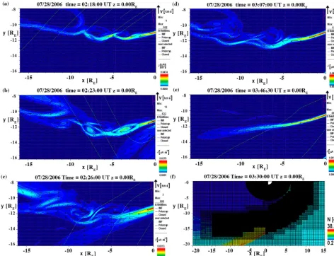
Figure 2.Figure from Hwang et al. (2011) where vortices were found using the BATS-R-US simulation. The region of the dawnside flank magnetopause is blown up (−16≤X(RE)≤0 and−16≤Y (RE)≤ −8), the current density is color-coded, and flow velocities are denoted
by arrows(a–e). The grid in theX–Y plane used for the simulation is shown in panel(f)where density is color-coded here.
2 Methodology
In this paper, we focus our attention on the simulation run employed by Hwang et al. (2011) to study Kelvin Helmholtz vortices during southward IMF. We acquired the 3-dimensional BATS-R-US model (Powell et al., 1999; Gombosi et al., 2004; Tóth et al., 2012) runs from the CCMC database (cdf files), interpolated to a uniform grid with cus-tom Python code using CCMC’s Kameleon library, and ex-tracted the velocity components to ingest into the custom an-alytics for vortex identification in our VIA. The code has run-time options for a search region bounding box, and a prefer-ential vorticity direction. We limited the region to that ref-erenced in Hwang’s study (−16RE< X <0RE, −16RE< Y <−8RE), and vorticity axis within 45◦of theZaxis. The algorithm then computes the velocity gradient tensor for each point in the flow field,∇v, which can be written as the sum of a symmetric partS=1/2(∇v+ ∇vT)and an
antisymmet-ric partR=1/2(∇v−∇vT).Scorresponds to the strain field
in the three dimensions of its eigenvectors.Rcorresponds to the rotation. If the norm ofRis greater than the norm ofS, we consider this point to lie at the center of a possible vor-tex, since the rotational strength magnitude exceeds the shear strain rate (Hunt et al., 1988).
clas-1120 Y. M. Collado-Vega et al.: Data mining for vortices
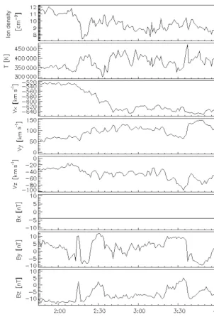
Figure 3.Solar wind conditions used for the MHD simulation used by Hwang et al. (2011). It shows the ion density, temperature,vx,vy,
vz,Bx,ByandBz.
sification. This new addition has been shown to help identify false positives, which is a capability that we did not have before. This method requires that at least 2 eigenvalues of S2+R2are negative. This algorithm is successful at finding the vortex center, but it is not immune to false hits. We can try to screen for these false hits by grouping the vortices into classes by spatial proximity. The class size can be used as a filter to eliminate isolated points that are more likely to be nu-merical artifacts. The vortex algorithm provides the location from which to begin, so the locations of interest are identi-fied faster, and they can be visualized using any available and compatible tool.
2.1 Analysis
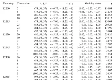
cur-Table 1.Properties of the vortices found with our algorithm separated into time step, cluster size, transformed coordinate system, vortex coordinates, vorticity vector andQvalue.
Time step Cluster size i,j,k x,y,z Vorticity vector Q
12200 5 (74, 56, 37) (−6.75,−11.25,−1) (0.05,−0.22,−0.97) 110 935 5 (75, 56, 37) (−6.50,−11.25,−1) (−0.01,−0.34,−0.94) 212 385 10 (86, 56, 37) (−3.75,−11.25,−1) (−0.07, 0.02,−1.00) 148 530 10 (87, 56, 37) (−3.50,−11.25,−1) (−0.07, 0.02,−1.00) 130 175 12215 4 (73, 56, 37) (−7.00,−11.25,−1) (0.00,−0.26,−0.96) 150 039 23 (83, 56, 37) (−4.50,−11.25,−1) (−0.01, 0.02,−1.00) 205 282 23 (84, 56, 37) (−4.25,−11.25,−1) (−0.01, 0.03,−1.00) 171 959 2 (97, 58, 37) (−1.00,−10.75,−1) (−0.02, 0.02,−1.00) 20 041 12230 30 (80, 56, 37) (−5.25,−11.25,−1) (0.02,−0.02,−1.00) 254 208 30 (81, 56, 37) (−5.00,−11.25,−1) (0.02,−0.02,−1.00) 249 727 9 (93, 57, 37) (−2.00,−11.00,−1) (0.00, 0.02,−1.00) 24 788 9 (94, 57, 37) (−1.75,−11.00,−1) (−0.07, 0.01,−1.00) 32 826 12245 25 (79, 56, 37) (−5.50,−11.25,−1) (−0.00,−0.05,−1.00) 257 976 4 (89, 56, 37) (−3.00,−11.25,−1) (−0.04, 0.01,−1.00) 39 254 4 (101, 59, 37) (0.00,−10.50,−1) (−0.02, 0.06,−1.00) 13 545 12300 26 (78, 56, 37) (−5.75,−11.25,−1) (0.00,−0.05,−1.00) 221 142 8 (88, 56, 37) (−3.25,−11.25,−1) (−0.03, 0.01,−1.00) 44 247 8 (89, 56, 37) (−3.00,−11.25,−1) (−0.07, 0.00,−1.00) 32 653 2 (66, 57, 37) (−8.75,−11.00,−1) (0.02,−0.15,−0.99) 80 514 4 (62, 58, 37) (−9.75,−10.75,−1) (−0.09,−0.20,−0.97) 18 026 3 (100, 59, 37) (−0.25,−10.50,−1) (0.07, 0.09,−0.99) 36 391 12315 4 (93, 57, 37) (−2.00,−11.00,−1) (0.01, 0.03,−1.00) 5398 4 (94, 57, 37) (−1.75,−11.00,−1) (0.03, 0.07,−1.00) 29 977
rent density, except in panel (f) where it represents the den-sity, and the arrows represent the flow direction. Some vor-tices can be seen starting to develop in diagram (a) around X= −4RE,Y = −10.8REandX= −7RE,Y = −11RE.
For several boundary crossing observations by Cluster, Hwang et al. (2011) tested the Kelvin–Helmholtz instabil-ity criteria for incompressible plasma conditions (Hasegawa, 1975) using the plasma and field parameters (Eq. 1). In this equation,v1,2represent flow velocity,ρ1,2the plasma mass density, and B1,2 magnetic field on sides 1 and 2, respec-tively. This equation indicates whether or not the interface is unstable to the instability, but not whether the instability de-velops nonlinearly. The results showed that the wave fronts observed during the different tested crossings were unstable to the Kelvin–Helmholtz instability and could grow nonlin-early.
BBk·(v2−v1)2
> 1 µ0
1
ρ1+
1
ρ2
h
BB(B1·k)2+BB(B2·k)2
i
(1)
Having already noted the location of the vortices deter-mined by Hwang et al. (2011), we used the same simulation results to test the data mining capability of our tool. Figure 3 shows the solar wind conditions used as input for the MHD simulation. It shows the ion density, temperature,vx,vy,vz, Bx,By andBz. For most of the time interval, the IMF is southward.
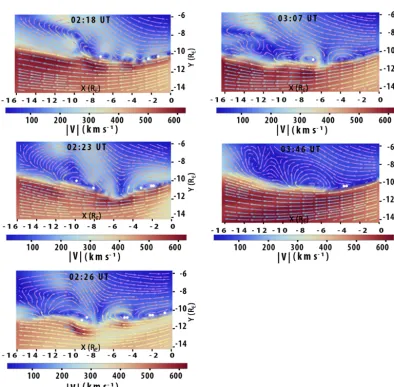
Table 1 displays in order the time step, the cluster size (group of vortices by spatial proximity), the local trans-formed coordinate system of the vorticity vector, the vortex coordinates in the geocentric solar magnetosphere (GSM), the vorticity vector and the value Q, the second invariant of the velocity gradient tensor which is used to identify points where the rotational strength exceeds the strain rate. A total of 86 179 vortex structures were detected (clusters, classes) with a mean of 345 for each time step for the data of 28 July 2006 from 02:15 to 03:55 UT. This covers the entire simulation space and includes vorticity vectors in all direc-tions (not preferentially in theZ direction). Figure 4 shows the vortices found using our data mining tool for the same time steps as those in Fig. 2. Looking at both figures, we can conclude that all vortices found by Hwang et al. (2011) are found by our data mining tool. The figure shows the vortex centers by a white dot and the velocity streamlines surround them with the colors corresponding to the velocity magni-tude. At 03:46 UT two rotations are visible with the stream-line at around X= −7RE, Y = −10RE and X= −13RE, Y= −8RE. These are vortices with centers near but not at theZ=0 cut plane shown in the figure.
[image:5.612.105.492.96.373.2]1122 Y. M. Collado-Vega et al.: Data mining for vortices
Figure 4.The white dots mark where the vortex centers were found using our VIA and they are visualized using Mathematica software for the same time steps as shown in Fig. 2. The colors represent velocity magnitude and the arrows indicate the flow direction.
Figure 5. 3-D representation of the vorticity vectors from the structure found on the Z=0 cut plane aroundX= −6.75RE and Y = −10.75RE(shown at the left). The tool can give more information on the extent of the vorticity vectors (shown in black screwlike
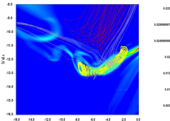
[image:6.612.61.532.508.661.2]Figure 6.Close-up view of a flux transfer event in the MHD simulation at 02:23 UTC (centered atX= −3.5REandY= −13RE) seen in
Fig. 2b. The color lines represent the magnetic field lines, with red being closed magnetic field lines, gray being “open” field lines (which are magnetic field lines connected on one side to Earth and on the other side to the solar wind), and yellow lines being those magnetic field lines of the IMF in the solar wind. This 2-D display shows the connectivity of the magnetic field lines of the flux transfer event.
Figure 7.3-D display of the FTE shown in Fig. 6. The solar mag-netic field lines of the flux transfer event on the X–Y plane are shown in the yellow color.
Kelvin–Helmholtz vortex. Figure 5 shows the 3-D represen-tation of this coherent structure with the vorticity vectors shown in black (middle figure) and where they are located in the magnetosphere, with theX,Y andZaxes represented in red, green and blue colors respectively. This shows that our findings are consistent with the assessment done by Hwang et al. (2011).
Hwang et al. (2011) described some of the vortical struc-tures seen in Fig. 2b as flux transfer events, which are tran-sient flux tubes that occur after magnetic reconnection on the dayside magnetopause. Any spacecraft encountering this flux tube would see a change in the magnetic field charac-teristics of the magnetopause boundary. These signatures are best described in boundary normal coordinates (LMN) to the magnetopause, which were first described by Russell and El-phic (1978). The flux tube exhibits bipolar signatures in the normal component of the magnetic field when these magne-tosheath field lines not connected to the magnetosphere drape over the connected flux tube (Le et al., 1993). The bipolar signatures normal to the magnetopause appear in both mag-netosheath and magnetospheric magnetic field lines draped over and under the FTE, because it bulges outward in both directions. They may also appear within the FTE itself, if there is a field-aligned current along the axis of the event. Saunders et al. (1984) showed evidence of such plasma vor-ticity within FTEs, which was attributed to an Alfvén wave propagating along the axis.
[image:7.612.45.290.391.554.2]1124 Y. M. Collado-Vega et al.: Data mining for vortices
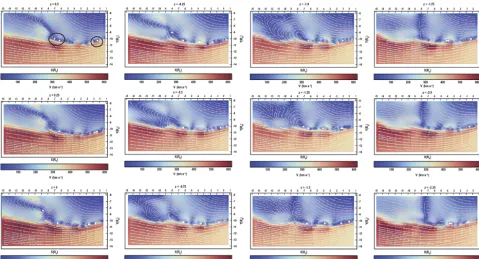
Figure 8.The extension along the Zaxis of the vortices and FTE presented in the time step of 02:18 UTC. The velocity magnitude is represented by the background color and streamlines are represented by arrows (left to right). The Kelvin–Helmholtz vortex and FTE are emphasized in the first panel by black circles. The white dots represent the center of the vortices as found by our algorithm. The FTE is still visible atZ= −2.25RE, whereas the Kelvin–Helmholtz vortex center is last seen atZ= −1.5RE.
of Fig. 2b. The color lines represent the magnetic field lines, with red being closed magnetic field lines, gray being “open” field lines (which are magnetic field lines connected on one side to Earth and on the other side to the solar wind), and yel-low lines being those magnetic field lines of the IMF in the solar wind. The figure shows that the vortical structure con-tains a mix of “open” magnetic field lines and magnetic field lines from the solar wind, so we infer that this structure is indeed a flux transfer event. Figure 7 shows the 3-D window display using the same visualization tool of the same struc-ture shown in Fig. 6, which shows the 3-D strucstruc-ture of the flux transfer event with the solar wind magnetic field lines shown in yellow color. This suggests that our tool can iden-tify not only vortices created by the Kelvin–Helmholtz in-stability but also FTEs, as long as they exhibit an internal vortical structure (Saunders et al., 1984).
To study the vortex properties in more depth, we visualized how the structure of the vortices changed in theZdirection, which is the axis of rotation for the targeted vortices. Figure 7 shows the extent of the FTE and vortices at the time step of 02:18 UTC from Hwang et al. (2011). The figure shows the 2-D image for the vortex structures found with the velocity magnitude represented in color. It covers fromZ=0.5REto Z= −2.25RE, showing the evolution of these vortical struc-tures along their axis of rotation. The Kelvin–Helmholtz vor-tex and FTE are emphasized on the first diagram by black
circles. It can be seen that the Kelvin–Helmholtz vortex is less extended than the FTE in this case. The FTE is still vis-ible atZ= −2.25RE, whereas the Kelvin–Helmholtz vortex center is last seen atZ= −1.5RE. This type of analysis mea-sures how large the vortices are, how they change temporally, and also how elongated they can be.
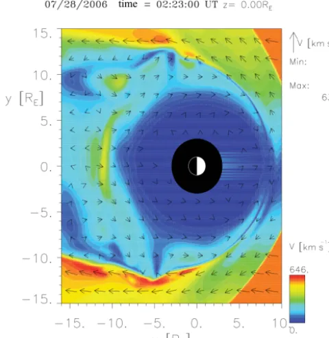
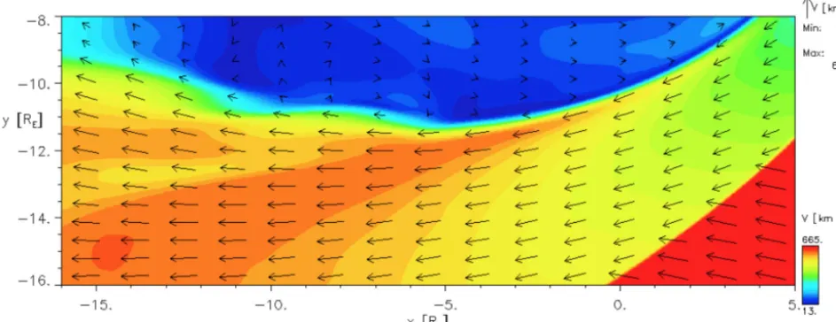
Figure 9.X–Y cut at 02:23 UTC showing velocity vectors super-posed on the velocity magnitude. It is observed that on the dawn-flank region nearby the observed vortices, the magnetosheath veloc-ity magnitude is higher than that observed in the solar wind outside the bow shock, higher than 600 km s−1. This diagram was made us-ing the visualization tool available online through the CCMC web-site.
2.2 Flow acceleration associated with vortices
Figure 9 shows flow velocity magnitudes at 02:23 UTC, when the vortex atX= −3.5REandY = −13REwas iden-tified. Magnetosheath velocities reach values higher than 600 km s−1near the vortex location, which is greater than the solar wind speed outside of the bow shock. Two questions arise: (1) is the Kelvin–Helmholtz vortex structure causing this kind of localized acceleration on the magnetosheath, or (2) is magnetic reconnection on the dayside causing these localized flow accelerations? Past studies have found mag-netosheath flow accelerating near the magnetopause when the IMF was northward. Phan et al. (1997) attributed this ac-celeration to the magnetic forces associated with draping of the field lines around the magnetopause. Chen et al. (1993) also proposed draping to be the source of the magnetosheath flow acceleration. On the other hand, Saunders et al. (1984) suggested that the presence of Kelvin–Helmholtz waves was made unstable due to the super-Alfvénic velocity shear oc-curring in reconnection accelerated flows under southward IMF. Our case is for southward IMF, and we see the accel-erated flows close to the magnetosheath side of the vortices found.
To determine whether the accelerated flows are only seen when the vortices are present, we need to compare times where vortices are found near the boundary with times when they are not. No vortex is visible in the diagram shown in Fig. 10 at the Z=0 cut plane using the visualization tool available through the CCMC website. However, speeds around the magnetosheath reach values similar to those in the solar wind speed, around 500–600 km s−1. The time step was run through our algorithm and some vortices were present nearby to the equatorial plane like the ones shown in Fig. 11 atZ=0.25RE (a) and atZ= −0.25RE (b). Consequently, the high-speed flows at the magnetopause are found to be as-sociated with the presence of vortices.
Figure 12 shows the flows at 03:55 UT (close to the end of the simulation run), when no vortex is visible on the bound-ary. This plot was made using the visualization tools avail-able online through the CCMC. Flow speeds are definitely high at the magnetopause as represented by the background color, but do not reach solar wind values as seen by the bow shock separation. This time step was searched by the double scrutiny test of the Lambda 2 method. No vortex was found in the vicinity of theZ=0 cut plane for this time step. Fig-ure 13 shows the output from our VIA where no vortex was found at theZ=0 cut plane.
These results could indicate that vortices could contribute to such localized acceleration as they convect antisunward. By contrast, Saunders et al. (1984) argued that the Kelvin– Helmholtz waves were driven by the super-Alfvénic shear created by the accelerated reconnected flows. In our case, flow is accelerated to speeds equal to or higher than the solar wind speed when vortices are present at the boundary. Pre-sumably, this type of plasma acceleration could be a com-bination of the Alfvénic outflow created by magnetic recon-nection and the presence of the Kelvin–Helmholtz vortices at the boundary. In Fig. 13 it is noticeable that the speed at the magnetosheath close to the boundary is not of the or-der of the solar wind speed, which in this case is around 650 km s−1, but slightly slower (about 480 to 500 km s−1). At the flank, the speeds are considered high for the magne-tosheath flow. Thus, the reconnection process could be ac-celerating the flow through the draping of the reconnected magnetic field lines, making the boundary unstable to the Kelvin–Helmholtz instability. The vortices can then develop and increase the acceleration even further. Inspection shows that the J×B force and the pressure gradient are higher when vortices are present. The pressure gradient forces are greater than theJ×Bforces, and consequently the acceler-ation seen in the magnetosheath is the fluid dynamic effect of enhanced flow velocities over ridges in the magnetopause surface. An animation with all the frames in the simula-tion referring to the same coordinates (−16RE< X <0RE,
1126 Y. M. Collado-Vega et al.: Data mining for vortices
Figure 10.Close-up of theX–Ycut at 03:46 UT time step of the simulation where it appears that there no vortices are formed at the boundary. The quantities represented are the same as in Fig. 9. The flow speeds along the boundary are still elevated compared to the flow speed of the solar wind.
3 Conclusions and future work
The large data sets that are now available through magneto-spheric simulations and also spacecraft missions require an automated search algorithm to focus on specific areas or fea-tures such as transients on the magnetopause boundary. It is really difficult to visually identify small-scale features in a 3-D vector field, both from the aspect of visualization and sheer data volume, without an automatic search algorithm like the one described in this paper.
We have leveraged a technique used in fluid dynamics to automatically detect vortical structure and elucidate its properties. The algorithm provides information on the 3-D properties and extent of the identified vortical structures. We have identified vortical structures not only attributed to the Kelvin–Helmholtz instability, but to flux transfer events. The magnetic topology seen in this vortical structures confirms this.
Our data demonstrate that the algorithm can identify vor-tical structures in a simulation based on solar wind condi-tions where Kelvin–Helmholtz vortices were found in obser-vations by the Cluster mission for southward IMF (Hwang et al., 2011). This is valuable feedback to the theory and sci-entific understanding of the phenomena, with the huge ad-vantage that the simulation data offer a high temporal- and spatial-resolution view. Our technique thus provides a means to exploit the high temporal and spatial resolution of simula-tion data and derive feature-specific informasimula-tion to feed back into the science discovery process.
We have also demonstrated that the Kelvin–Helmholtz vortices, analyzed and formed under southward IMF for the case shown, are associated with the accelerated flows
ob-served on the magnetosheath side, with speeds higher than the solar wind speed observed at the bow shock. No such ac-celerated flows were visible when no vortices were present at the boundary. These accelerated flows can be attributed to the draping of the magnetic field lines in conjunction with the super-Alfvénic shear occurring at the boundary due to the Kelvin–Helmholtz vortices. Inspection shows that theJ×B force and the pressure gradient are higher when the vortices are present.
In the near future, we plan to leverage this capability to in-clude the magnetic field topology and delve into the specific vortex characteristics to increase the science return from the data. We also want to compare the simulation results with in situ observations by different spacecraft data for algo-rithm validation. One promising application of our VIA is the possibility to search vortical structures in data from mis-sions like the Magnetospheric Multiscale Mission (MMS), in which four satellites fly in a tetrahedral formation with a small separation.
Data availability. Simulation results were provided by the Com-munity Coordinated Modeling Center at Goddard Space Flight Center through their public Runs on Request system (http://ccmc. gsfc.nasa.gov). The Block-Adaptive-Tree-Solarwind-Roe-Upwind-Scheme (BATS-R-US; ID KyoungJoo_Hwang_101309_1a) Model was developed by Tamas Gombosi et al. at the Center for Space Environment Modeling, University of Michigan.
Figure 11. With our algorithm we find that there are vortices present at theZ=0.25RE (a)and the Z= −0.25RE coordinate(b) at
03:46 UTC. The center of the vortices is represented by the white dots.
Author contributions. YMCV wrote the manuscript, helped with the algorithm development and analyzed the algorithm output data. VLK developed the algorithm, processed the simulation data, cre-ated custom visualizations for the algorithm results, and helped with the editing of the manuscript. DGS helped with the analysis and
editing of the manuscript. KJH is the author of a previous analysis used in the paper. LR helped with the simulations used.
1128 Y. M. Collado-Vega et al.: Data mining for vortices
Figure 12.Close-up of theX–Y cut at 03:55 UTC when no vortex is visible. Quantities shown are the same as the ones in Fig. 9. The flow speeds along the boundary are not as high as those on the solar wind.
Figure 13.Output from our code that shows the velocity magnitude as the background color with no vortices detected at 03:55 UTC on the
X–Y plane or close by.
Acknowledgements. This work was supported by the FY2015 Science Innovation Fund from NASA Headquarters. The authors would like to thank Jay Friedlander for his amazing help with the manuscript figures.
The topical editor, Elias Roussos, thanks two anonymous referees for help in evaluating this paper.
References
Chen, S.-H., Kivelson, M. G., Gosling, J. T., Walker, R. J., and Lazarus, A. J.: Anomalous aspects of magnetosheath flow and of the shape and oscillations of the magnetopause during an interval of strongly northward interplanetary magnetic field, J. Geophys. Res., 98, 5727–5742, 1993.
[image:12.612.106.486.298.560.2]vor-tices observed during high-speed streams, J. Geophys. Res., 112, A06213, https://doi.org/10.1029/2006JA012104, 2007.
Collado-Vega, Y. M., Kessel, R. L., Sibeck, D. G., Kalb, V. L., Boller, R. A., and Rastaetter, L.: Comparison be-tween vortices created and evolving during fixed and dy-namic solar wind conditions, Ann. Geophys., 31, 1463–1483, https://doi.org/10.5194/angeo-31-1463-2013, 2013.
Fujimoto, M., Tonooka, T., and Mukai, T.: Vortex-Like Fluctuations in the Magnetotail Flanks and their Possible Roles in Plasma Transport, in Earth’s Low-Latitude Boundary Layer, American Geophysical Union, 2003.
Gombosi, T. I., Powell, K. G., De Zeeuw, D. L., Clauer, C. R., Hansen, K. C., Manchester, W. B., Ridley, A. J., Roussev, I. I., Sokolov, I. V., Stout, Q. F., and Toth, G.: Solution-adaptive mag-netohydrodynamics for space plasmas: Sun-to-Earth simulations, Comput. Sci. Eng., 6, 14–35, 2004.
Hasegawa, A.: Plasma Instabilities and Nonlinear Effects, Springer, Verlag, 1975.
Hasegawa, H., Fujimoto, M., Phan, T.-D., Rème, H., Balogh, A., Dunlop, M. W., Hashimoto, C., and TanDokoro, R.: Transport of solar wind into Earth’s magnetosphere through rolled-up Kelvin-Helmholtz vortices, Nature, 430, 755–758, 2004a.
Hasegawa, H., Fujimoto, M., Takagi, K., Saito, Y., Mukai, T., and Rème, H.: Single-spacecraft detection of rolled-up Kelvin-Helmholtz vortices at the flank magnetopause, J. Geophys. Res., 111, A09203, https://doi.org/10.1029/2006JA011728, 2006. Hunt, J., Wiley, A., and Moin, P.: Eddies, Stream, and Convergence
Zones in Turbulent Flows, Studying Turbulence Using Numeri-cal Simulation Databases, 1, 193–208, 1988.
Hwang, K.-J., Kuznetsova, M. M., Sahraoui, F., Goldstein, M. L., Lee, E., and Parks, G. K.: Kelvin-Helmholtz waves under southward interplanetary magnetic field, J. Geophys. Res., 116, A08210, https://doi.org/10.1029/2011JA016596, 2011.
Hwang, K.-J., Goldstein, M. L., Kuznetsova, M. M., Wang, Y., Viñas, A. F., and Sibeck, D. G.: The first in situ ob-servation of Kelvin-Helmholtz waves at high-latitude netopause during strongly dawnward interplanetary mag-netic field conditions, J. Geophys. Res., 117, A08233, https://doi.org/10.1029/2011JA017256, 2012.
Jeong, J. and Hussain, F.: On the Identification of a Vortex, J. Fluid Mech., 285, 69–94, 1995.
Kavosi, S. and Raeder, J.: Ubiquity of Kelvin–Helmholtz waves at Earth’s magnetopause, Nat. Commun., 6, 7019, https://doi.org/10.1038/ncomms8019, 2015.
Kivelson, M. G. and Chen, S. H.: The Magnetopause: Surface waves and instabilities and their possible dynamical consequences, vol. 90 of Geophys. Monogr. Ser., chap. Physics of the Magne-topause, American Geophysical Union, 257–268, 1995. Le, G., Russell, C. T., and Kuo, H.: Flux transfer events:
sponta-neous or driven?, Geophys. Res. Lett., 20, 791–794, 1993. Miura, A.: Anomalous transport by magnetohydrodynamic
Kelvin-Helmholtz instabilities in the solar wind-magnetosphere interac-tion, J. Geophys. Res., 89, 801–818, 1984.
Nakamura, T. and Fujimoto, M.: Magnetic reconnection within MHD-scale KelvHelmholtz vortices triggered by electron in-ertial effects, Elsevier, 37, 522–526, 2006.
Nykyri, K. and Otto, A.: Plasma transport at the magnetospheric boundary due to reconnection in Kelvin-Helmholtz vortices, Geophys. Res. Lett., 28, 3565–3568, 2001.
Phan, T. D., Larson, D., McFadden, J., Lin, R. P., Carlson, C., Moyer, M., and Paularena, K. I.: Low-latitude dusk flank mag-netosheath, magnetopause, and boundary layer for low magnetic shear: Wind observations, J. Geophys. Res., 102, 19883–19895, 1997.
Powell, K., Roe, P., Linde, T., Gombosi, T. I., and Zeeuw, D. L. D.: A solution-adaptive upwind scheme for ideal magnetohydrody-namics, J. Comp. Phys., 154, 284–309, 1999.
Russell, C. T. and Elphic, R. C.: Initial ISEE magnetometer results: Magnetopause observations, Space Sci. Rev., 22, 681–715, 1978. Saunders, M. A., Russell, C. T., and Sckopke, N.: Flux transfer events: Scale size and interior structure, Geophys. Res. Lett., 11, 131–134, 1984.
Takagi, K., Hashimoto, C., Hasegawa, H., Fujimoto, M., and Tan-Dokoro, R.: Kelvin-Helmholtz instability in a magnetotail flank-like geometry: Three dimensional MHD simulations, J. Geophys. Res., 111, A08202, https://doi.org/10.1029/2006JA011631, 2006.