TOWARDS EFFICIENT COMPILATION OF THE HPJAVA LANGUAGE FOR HIGH PERFORMANCE COMPUTING
Name: Han-Ku Lee
Department: Department of Computer Science Major Professor: Gordon Erlebacher
Degree: Doctor of Philosophy
Term Degree Awarded: Summer, 2003
This dissertation is concerned with efficient compilation of our Java-based, high-performance, library-oriented, SPMD style, data parallel programming language: HPJava.
It starts with some historical review of data-parallel languages such as High Performance Fortran (HPF), message-passing frameworks such as p4, PARMACS, and PVM, as well as the MPI standard, and high-level libraries for multiarrays such as PARTI, the Global Array (GA) Toolkit, and Adlib.
we discuss optimization strategies we will apply such as Partial Redundancy Elimination, Strength Reduction, Dead Code Elimination, and Loop Unrolling. We experiment with and benchmark large scientific and engineering HPJava programs on Linux machine, shared memory machine, and distributed memory machine to prove our compilation and proposed optimization schemes are appropriate for the HPJava system.
THE FLORIDA STATE UNIVERSITY
COLLEGE OF ARTS AND SCIENCES
TOWARDS EFFICIENT COMPILATION OF THE HPJAVA LANGUAGE FOR HIGH PERFORMANCE COMPUTING
By
HAN-KU LEE
A Dissertation submitted to the Department of Computer Science
in partial fulfillment of the requirements for the degree of
Doctor of Philosophy
The members of the Committee approve the dissertation of Han-Ku Lee defended on June 12, 2003.
Gordon Erlebacher
Professor Directing Thesis
Larry Dennis
Outside Committee Member
Geoffrey C. Fox Committee Member
Michael Mascagni Committee Member
Daniel Schwartz Committee Member
To my mother, father, big sisters, and all my friends . . .
ACKNOWLEDGEMENTS
TABLE OF CONTENTS
List of Tables . . . viii
List of Figures . . . x
Abstract. . . xiii
1. INTRODUCTION . . . 1
1.1 Research Objectives . . . 1
1.2 Organization of This Dissertation . . . 2
2. BACKGROUND. . . 4
2.1 Historical Review of Data Parallel Languages . . . 4
2.1.1 Multi-processing and Distributed Data . . . 6
2.2 High Performance Fortran . . . 9
2.2.1 The Processor Arrangement and Templates . . . 10
2.2.2 Data Alignment . . . 12
2.3 Message-Passing for HPC . . . 15
2.3.1 Overview and Goals . . . 15
2.3.2 Early Message-Passing Frameworks . . . 15
2.3.3 MPI: A Message-Passing Interface Standard . . . 17
2.4 High Level Libraries for Distributed Arrays . . . 19
2.4.1 PARTI . . . 20
2.4.2 The Global Array Toolkit . . . 22
2.4.3 NPAC PCRC Runtime Kernel – Adlib . . . 22
2.5 Discussion . . . 23
3. THE HPSPMD PROGRAMMING MODEL . . . 25
3.1 Motivations . . . 25
3.2 HPspmd Language Extensions . . . 26
3.3 Integration of High-Level Libraries . . . 27
3.4 The HPJava Language . . . 28
3.4.1 Multiarrays . . . 28
3.4.2 Processes . . . 29
3.4.3 Distributed Arrays . . . 31
3.4.4 Parallel Programming and Locations . . . 33
3.4.5 More Distribution Formats . . . 36
3.4.6 Array Sections . . . 45
3.4.7 Low Level SPMD Programming . . . 49
3.6 Discussion . . . 53
4. COMPILATION STRATEGIES FOR HPJAVA . . . 55
4.1 Multiarray Types and HPspmd Classes . . . 55
4.2 Abstract Syntax Tree . . . 58
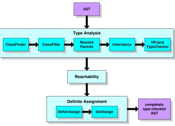
4.3 Type-Checker . . . 59
4.3.1 Type Analysis . . . 61
4.3.2 Reachability and Definite (Un)assignment Analysis . . . 62
4.4 Pre-translation . . . 64
4.5 Basic Translation Scheme . . . 66
4.5.1 Translation of a multiarray declaration . . . 67
4.5.2 Translation of multiarray creation . . . 70
4.5.3 Translation of the on construct . . . 70
4.5.4 Translation of the at construct . . . 71
4.5.5 Translation of the overall construct . . . 72
4.5.6 Translation of element access in multiarrays . . . 74
4.5.7 Translation of array sections . . . 75
4.5.7.1 Simple array section – no scalar subscripts . . . 75
4.5.7.2 Integer subscripts in sequential dimensions . . . 76
4.5.7.3 Scalar subscripts in distributed dimensions . . . 77
4.6 Test Suites . . . 78
4.7 Discussion . . . 79
5. OPTIMIZATION STRATEGIES FOR HPJAVA. . . 80
5.1 Partial Redundancy Elimination . . . 80
5.2 Strength Reduction . . . 83
5.3 Dead Code Elimination . . . 85
5.4 Loop Unrolling . . . 85
5.5 Applying PRE, SR, DCE, and LU . . . 86
5.5.1 Case Study: Direct Matrix Multiplication . . . 87
5.5.2 Case Study: Laplace Equation Using Red-Black Relaxation . . . 89
5.6 Discussion . . . 93
6. BENCHMARKING HPJAVA, PART I: NODE PERFORMANCE. . . 95
6.1 Importance of Node Performance . . . 96
6.2 Direct Matrix Multiplication . . . 97
6.3 Partial Differential Equation . . . 99
6.3.1 Background on Partial Differential Equations . . . 99
6.3.2 Laplace Equation Using Red-Black Relaxation . . . 100
6.3.3 3-Dimensional Diffusion Equation . . . 104
6.4 Q3 – Local Dependence Index . . . 106
6.4.1 Background on Q3 . . . 106
6.4.2 Data Description . . . 107
6.4.3 Experimental Study – Q3 . . . 107
7. BENCHMARKING HPJAVA, PART II:
PERFORMANCE ON PARALLEL MACHINES . . . .112
7.1 Direct Matrix Multiplication . . . 113
7.2 Laplace Equation Using Red-Black Relaxation . . . 115
7.3 3-Dimensional Diffusion Equation . . . 120
7.4 Q3 – Local Dependence Index . . . 121
7.5 Discussion . . . 124
8. RELATED SYSTEMS. . . .125
8.1 Co-Array Fortran . . . 125
8.2 ZPL . . . 126
8.3 JavaParty . . . 127
8.4 Timber . . . 129
8.5 Titanium . . . 131
8.6 Discussion . . . 132
9. CONCLUSIONS . . . .133
9.1 Conclusion . . . 133
9.2 Contributions . . . 134
9.3 Future Works . . . 135
9.3.1 HPJava . . . 135
9.3.2 High-Performance Grid-Enabled Environments . . . 135
9.3.2.1 Grid Computing Environments . . . 135
9.3.2.2 HPspmd Programming Model Towards Grid-Enabled Applications 136 9.3.3 Java Numeric Working Group from Java Grande . . . 138
9.3.4 Web Service Compilation (i.e. Grid Compilation) . . . 138
9.4 Current Status of HPJava . . . 140
9.5 Publications . . . 141
REFERENCES. . . .143
LIST OF TABLES
6.1 Compilers and optimization options lists used on Linux machine. . . 96 6.2 Speedup of each application over naive translation and sequential Java after
applying HPJOPT2. . . 111 7.1 Compilers and optimization options lists used on parallel machines. . . 113 7.2 Speedup of the naive translation over sequential Java and C programs for the
direct matrix multiplication on SMP. . . 113 7.3 Speedup of the naive translation and PRE for each number of processors over
the performance with one processor for the direct matrix multiplication on SMP. . . 114 7.4 Speedup of the naive translation over sequential Java and C programs for the
Laplace equation using red-black relaxation without Adlib.writeHalo() on SMP. . . 116 7.5 Speedup of the naive translation and HPJOPT2 for each number of processors
over the performance with one processor for the Laplace equation using red-black relaxation without Adlib.writeHalo() on SMP. . . 117 7.6 Speedup of the naive translation over sequential Java and C programs for the
Laplace equation using red-black relaxation on SMP. . . 118 7.7 Speedup of the naive translation and HPJOPT2 for each number of processors
over the performance with one processor for the Laplace equation using red-black relaxation on SMP. . . 118 7.8 Speedup of the naive translation for each number of processors over the
performance with one processor for the Laplace equation using red-black relaxation on the distributed memory machine. . . 119 7.9 Speedup of the naive translation over sequential Java and C programs for the
3D Diffusionequation on the shared memory machine. . . 121 7.10 Speedup of the naive translation and HPJOPT2 for each number of processors
over the performance with one processor for the 3D Diffusion equation on the shared memory machine. . . 121 7.11 Speedup of the naive translation for each number of processors over the
performance with one processor for the 3D diffusion equation on the distributed memory machine. . . 121 7.12 Speedup of the naive translation over sequential Java and C programs for Q3
LIST OF FIGURES
2.1 Idealized picture of a distributed memory parallel computer . . . 6
2.2 A data distribution leading to excessive communication . . . 7
2.3 A data distribution leading to poor load balancing . . . 8
2.4 An ideal data distribution . . . 9
2.5 Alignment of the three arrays in the LU decomposition example . . . 13
2.6 Collective communications with 6 processes. . . 19
2.7 Simple sequential irregular loop. . . 20
2.8 PARTI code for simple parallel irregular loop. . . 21
3.1 The process grids illustrated by p . . . 30
3.2 The Group hierarchy of HPJava. . . 30
3.3 The process dimension and coordinates in p. . . 31
3.4 A two-dimensional array distributed over p. . . 32
3.5 A parallel matrix addition. . . 33
3.6 Mapping of x and y locations to the gridp. . . 35
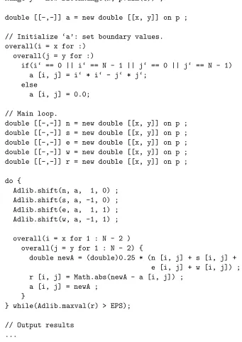
3.7 Solution for Laplace equation by Jacobi relaxation in HPJava. . . 37
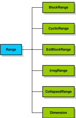
3.8 The HPJava Range hierarchy. . . 38
3.9 Work distribution for block distribution. . . 39
3.10 Work distribution for cyclic distribution. . . 39
3.11 Solution for Laplace equation using red-black with ghost regions in HPJava. . . 41
3.12 A two-dimensional array, a, distributed over one-dimensional grid, q. . . 42
3.13 A direct matrix multiplication in HPJava. . . 43
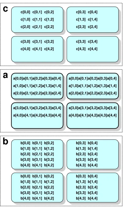
3.14 Distribution of array elements in example of Figure 3.13. Arraya is replicated in every column of processes, array b is replicated in every row. . . 44
3.15 A general matrix multiplication in HPJava. . . 45
3.16 A one-dimensional section of a two-dimensional array (shaded area). . . 47
3.17 A two-dimensional section of a two-dimensional array (shaded area). . . 47
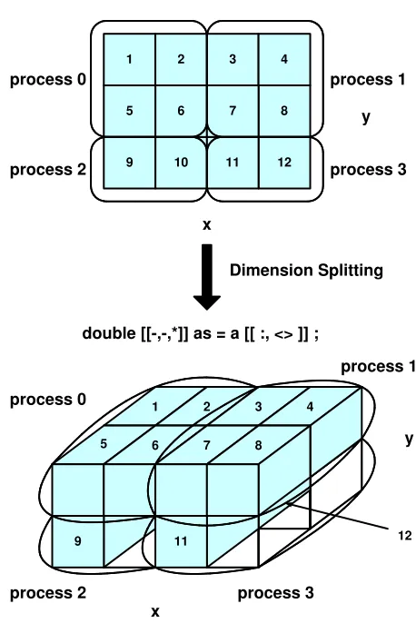
3.19 N-body force computation using dimension splitting in HPJava. . . 51
3.20 The HPJava Architecture. . . 54
4.1 Part of the lattice of types for multiarrays of int. . . 56
4.2 Example of HPJava AST and its nodes. . . 59
4.3 Hierarchy for statements. . . 60
4.4 Hierarchy for expressions. . . 60
4.5 Hierarchy for types. . . 60
4.6 The architecture of HPJava Front-End. . . 61
4.7 Example source program before pre-translation. . . 65
4.8 Example source program after pre-translation. . . 66
4.9 Translation of a multiarray-valued variable declaration. . . 68
4.10 Translation of multiarray creation expression. . . 69
4.11 Translation ofon construct. . . 71
4.12 Translation ofat construct. . . 72
4.13 Translation ofoverall construct. . . 73
4.14 Translation of multiarray element access. . . 74
4.15 Translation of array section with no scalar subscripts. . . 75
4.16 Translation of array section without any scalar subscripts indistributed dimen-sions. . . 77
4.17 Translation of array section allowing scalar subscripts in distributed dimensions. 78 5.1 Partial Redundancy Elimination . . . 81
5.2 Simple example of Partial Redundancy of loop-invariant . . . 82
5.3 Before and After Strength Reduction . . . 83
5.4 Translation of overall construct, applying Strength Reduction. . . 84
5.5 The innermost for loop of naively translated direct matrix multiplication . . . 87
5.6 Inserting a landing pad to a loop . . . 87
5.7 After applying PRE to direct matrix multiplication program . . . 88
5.8 Optimized HPJava program of direct matrix multiplication program by PRE and SR . . . 89
5.9 The innermost overall loop of naively translated Laplace equation using red-black relaxation . . . 90
6.1 Performance for Direct Matrix Multiplication in HPJOPT2, PRE, Naive
HPJava, Java, and C on the Linux machine . . . 98
6.2 Performance comparison between 150 × 150 original Laplace equation from Figure 3.11 and split version of Laplace equation. . . 102
6.3 Memory locality for loop unrolling and split versions. . . 103
6.4 Performance comparison between 512 × 512 original Laplace equation from Figure 3.11 and split version of Laplace equation. . . 104
6.5 3D Diffusion Equation in Naive HPJava, PRE, HPJOPT2, Java, and C on Linux machine . . . 105
6.6 Q3 Index Algorithm in HPJava . . . 108
6.7 Performance for Q3 on Linux machine . . . 109
7.1 Performance for Direct Matrix Multiplication on SMP. . . 114
7.2 512×512 Laplace Equation using Red-Black Relaxation withoutAdlib.writeHalo() on shared memory machine . . . 116
7.3 Laplace Equation using Red-Black Relaxation on shared memory machine . . . 117
7.4 Laplace Equation using Red-Black Relaxation on distributed memory machine 119 7.5 3D Diffusion Equation on shared memory machine . . . 120
7.6 3D Diffusion Equation on distributed memory machine . . . 122
7.7 Q3 on shared memory machine . . . 123
8.1 A simple Jacobi program in ZPL. . . 128
ABSTRACT
This dissertation is concerned with efficient compilation of our Java-based, high-performance, library-oriented, SPMD style, data parallel programming language: HPJava.
It starts with some historical review of data-parallel languages such as High Performance Fortran (HPF), message-passing frameworks such as p4, PARMACS, and PVM, as well as the MPI standard, and high-level libraries for multiarrays such as PARTI, the Global Array (GA) Toolkit, and Adlib.
Next, we will introduce our own programming model, which is a flexible hybrid of HPF-like data-parallel language features and the popular, library-oriented, SPMD style. We refer to this model as the HPspmd programming model. We will overview the motivation, the language extensions, and an implementation of our HPspmd programming language model, called HPJava. HPJava extends the Java language with some additional syntax and pre-defined classes for handling multiarrays, and a few new control constructs. We discuss the compilation system, including HPspmd classes, type-analysis, pre-translation, and basic translation scheme. In order to improve the performance of the HPJava system, we discuss optimization strategies we will apply such as Partial Redundancy Elimination, Strength Reduction, Dead Code Elimination, and Loop Unrolling. We experiment with and benchmark large scientific and engineering HPJava programs on Linux machine, shared memory machine, and distributed memory machine to prove our compilation and proposed optimization schemes are appropriate for the HPJava system.
CHAPTER 1
INTRODUCTION
1.1
Research Objectives
Historically, data parallel programming and data parallel languages have played a major role in high-performance computing. By now we know many of the implementation issues, but we remain uncertain what the high-level programming environment should be. Ten years ago the High Performance Fortran Forum published the first standardized definition of a language for data parallel programming. Since then, substantial progress has been achieved in HPF compilers, and the language definition has been extended because of the requests of compiler-writers and the end-users. However, most parallel application developers today don’t use HPF. This does not necessarily mean that most parallel application developers prefer the lower-level SPMD programming style. More likely, we suggest, it is either a problem with implementations of HPF compilers, or rigidity of the HPF programming model. Research on compilation technique for HPF continues to the present time, but efficient compilation of the language seems still to be an incompletely solved problem. Meanwhile, many successful applications of parallel computing have been achieved by hand-coding parallel algorithms using low-level approaches based on the libraries like Parallel Virtual Machine (PVM), Message-Passing Interface (MPI), and Scalapack.
common operations such as distributed parallel loops. Unlike HPF, but similar to MPI, communication is always explicit. Thus, irregular patterns of access to array elements can be handled by making explicit bindings to libraries.
The major goal of the system we are building is to provide a programming model which is a flexible hybrid of HPF-like data-parallel language and the popular, library-oriented, SPMD style. We refer to this model as the HPspmd programming model. It incorporates syntax for representing multiarrays, for expressing that some computations are localized to some processors, and for writing a distributed form of the parallel loop. Crucially, it also supports binding from the extended languages to various communication and arithmetic libraries. These might involve simply new interfaces to some subset of PARTI, Global Arrays, Adlib, MPI, and so on. Providing libraries for irregular communication may well be important. Evaluating the HPspmd programming model on large scale applications is also an important issue.
What would be a good candidate for the base-language of our HPspmd programming model? We need a base-language that is popular, has the simplicity of Fortran, enables modern object-oriented programming and high performance computing with SPMD libraries, and so on. Java is an attractive base-language for our HPspmd model for several reasons: it has clean and simple object semantics, cross-platform portability, security, and an increasingly large pool of adept programmers. Our research aim is to power up Java for the data parallel SPMD environment. We are taking on a more modest approach than a full scale data parallel compiler like HPF. We believe this is a proper approach to Java where the situation is rapidly changing and one needs to be flexible.
1.2
Organization of This Dissertation
We will survey the history and recent developments in the field of programming languages and environments for data parallel programming. In particular, we describe ongoing work at Florida State University and Indiana University, which is developing a compilation system for a data parallel extension of the Java programming language.
(HPF) in the 1990s. We will review essential features of the HPF language and issues related to its compilation.
The second part of the dissertation is about the HPspmd programming model, including the motivation, HPspmd language extensions, integration of high-level libraries, and an example of the HPspmd model in Java—HPJava.
The third part of the dissertation covers background and current status of the HPJava compilation system. We will describe the multiarray types and HPspmd classes, basic translation scheme, and optimization strategies.
The fourth part of the dissertation is concerned with experimenting and benchmarking some scientific and engineering applications in HPJava, to prove the compilation and optimization strategies we will apply to the current system are appropriate.
The fifth part of the dissertation compares and contrasts with modern related languages including Co-Array Fortran, ZPL, JavaParty, Timber, and Titanium. Co-Array Fortran is an extended Fortran dialect for SPMD programming; ZPL is an array-parallel programming language for scientific computations; JavaParty is an environment for cluster-based parallel programming in Java; Timber is a Java-based language for array-parallel programming. Titanium is a language and system for high-performance parallel computing, and its base language is Java; We will describe the systems and discuss the relative advantages of our proposed system.
CHAPTER 2
BACKGROUND
2.1
Historical Review of Data Parallel Languages
Many computer–related scientists and professionals will probably agree with the idea that, in a short time—less than decade—every PC will have multi-processors rather than uni-processors1. This implies that parallel computing plays a critically important role not only in scientific computing but also the modern computer technology.
There are lots of places where parallel computing can be successfully applied— supercomputer simulations in government labs, scaling Google’s core technology powered by the world’s largest commercial Linux cluster (more than 10,000 servers), dedicated clusters of commodity computers in a Pixar RenderFarm for animations [43, 39]. Or by collecting cycles of many available processors over Internet. Some of the applications involve large-scale “task farming,” which is applicable when the task can be completely divided into a large number of independent computational parts. The other popular form of massive parallelism is “data parallelism.” The term data parallelism is applied to the situation where a task involves some large data-structures, typically arrays, that are split across nodes. Each node performs similar computations on a different part of the data structure. For data parallel computation to work best, it is very important that the volume of communicated values should be small compared with the volume of locally computed results. Nearly all successful applications of massive parallelism can be classified as either task farming or data parallel.
For task farming, the level of parallelism is usually coarse-grained. This sort of parallel programming is naturally implementable in the framework of conventional sequential programming languages: a function or a method can be an abstract task, a library
1
can provide an abstract, problem-independent infrastructure for communication and load-balancing. For data parallelism, we meet a slightly different situation. While it is possible to code data parallel programs for modern parallel computers in ordinary sequential languages supported by communication libraries, there is a long and successful history of special languages for data parallel computing. Why is data parallel programming special?
Historically, a motivation for the development of data parallel languages is strongly related with Single Instruction Multiple Data (SIMD) computer architectures. In a SIMD computer, a single control unit dispatches instructions to large number of compute nodes, and each node executes the same instruction on its own local data.
The early data parallel languages developed for machines such as the Illiac IV and the ICL DAP were very suitable for efficient programming by scientific programmers who would not use a parallel assembly language. They introduced a new programming language concept—distributed or parallel arrays—with different operations from those allowed on sequential arrays.
In the 1980s and 1990s microprocessors rapidly became more powerful, more available, and cheaper. Building SIMD computers with specialized computing nodes gradually became less economical than using general purpose microprocessors at every node. Eventually SIMD computers were replaced almost completely by Multiple Instruction Multiple Data (MIMD) parallel computer architectures. In MIMD computers, the processors are autonomous: each processor is a full-fledged CPU with both a control unit and an ALU. Thus each processor is capable of executing its own program at its own pace at the same time: asynchronously.
Processors
Memory Area
Figure 2.1. Idealized picture of a distributed memory parallel computer
Soon a general approach was proposed in order to write data parallel programs for MIMD computers, having some similarities to programming SIMD computers. It is known as Single Program Multiple Data (SPMD) programming or the Loosely Synchronous Model. In SPMD, each node executes essentially the same thing at essentially the same time, but without any single central control unit like a SIMD computer. Each node has its own local copy of the control variables, and updates them in an identical way across MIMD nodes. Moreover, each node generally communicates with others in well-defined collective phases. These data communications implicitly or explicitly2 synchronize the nodes. This aggregate synchronization is easier to deal with than the complex synchronization problems of general concurrent programming. It was natural to think that catching the SPMD model for programming MIMD computers in data parallel languages should be feasible and perhaps not too difficult, like the successful SIMD languages. Many distinct research prototype languages experimented with this, with some success. The High Performance Fortran (HPF) standard was finally born in the 90s.
2.1.1 Multi-processing and Distributed Data
Figure 2.1 represents many successful parallel computers obtainable at the present time, which have a large number of autonomous processors, each possessing its own local memory area. While a processor can very rapidly access values in its own local memory, it must access values in other processors’ memory either by special machine instructions or message-passing software. But the current technology can’t make remote memory accesses nearly as fast as local memory accesses. Who then should get rid of this burden to minimize the number of
2
Processors
Memory Area
Parallel sub-calculation
Figure 2.2. A data distribution leading to excessive communication
accesses to non-local memory? The programmer or compiler? This is the communication problem.
A next problem comes from ensuring each processor has a fair share of the whole work load. We absolutely lose the advantage of parallelism if one processor, by itself, finishes almost all the work. This is the load-balancing problem.
High Performance Fortran (HPF) for example allows the programmer to add various directives to a program in order to explicitly specify the distribution of program data among the memory areas associated with a set of (physical or virtual) processors. The directives don’t allow the programmer to directly specify which processor will perform a specific computation. The compiler must decide where to do computations. We will see in chapter 3 that HPJava takes a slightly different approach but still requires programmers to distribute data.
We can think of some particular situation where all operands of a specific sub-computation, such as an assignment, reside on the same processor. Then, the compiler can allocate that part of the computation to the processor having the operands, and no remote memory access will be needed. So an onus on parallel programmers is to distribute data across the processors in the following ways:
Processors
Memory Area
Parallel sub-calculation
Figure 2.3. A data distribution leading to poor load balancing
• to maximize parallelism, the group ofdistinct sub-computations which can execute in parallel at any time should involve data on as many different processors as possible.
Sometimes these are contradictory goals. Highly parallel programs can be difficult to code and distribute efficiently. But, equally often it is possible to meet the goals successfully.
Suppose that we have an ideal situation where a program contains p sub-computations which can be executed in parallel. They might be pbasic assignments consisting of an array assignment or FORALL construct. Assume that each expression which is computed combines two operands. Including the variable being assigned, a single sub-computation therefore has three operands. Moreover, assume that there are p processors available. Generally, the number of processors and the number of sub-computations are probably different, but this is a simplified situation.
Figure 2.2 depicts that all operands of each sub-computation are allocated in different memory areas. Wherever the computation is executed, each assignment needs at least two communications.
Processors
Memory Area
Parallel sub-calculation
Figure 2.4. An ideal data distribution
Figure 2.4 depicts that all operands of an individual assignment occur on the same pro-cessor, but each group of the sub-computations is uniformly well-distributed over processors. In this case, we can depend upon the compiler to allocate each computation to the processor holding the operands, requiring no communication, and perfect distribution of the work load. Except in the most simple programs, it is impossible to choose a distribution of program variables over processors like Figure 2.4. The most important thing in distributed memory programming is to distribute the most critical regions of the program over processors to make them as much like Figure 2.4 as possible.
2.2
High Performance Fortran
Since then, except a few vendors like Portland, many of those still in business have given up their HPF projects. The goals of HPF were immensely aspiring, and perhaps attempted to put too many ideas into one language. Nevertheless, we think that many of the originally defined goals for HPF standardization of a distributed data model for SPMD computing are important.
2.2.1 The Processor Arrangement and Templates
The programmer often wishes to explicitly distribute program variables over the memory areas with respect to a set of processors. Then, it is desirable for a program to have some representations of the set of processors. This is done by the PROCESSORS directive.
The syntax of a PROCESSOR definition looks like the syntax of an array definition of Fortran:
!HPF$ PROCESSORS P (10)
This is a declaration of a set of 10 abstract processors, named P. Sets of abstract processors, orprocessor arrangements, can be multi-dimensional. For instance,
!HPF$ PROCESSORS Q (4, 4)
declares 16 abstract processors in a 4×4 array.
The programmer may directly distribute data arrays over processors. But it is often more satisfactory to go through the intermediate of an explicit template. Templates are different from processor arrangements. The collection of abstract processors in an HPF processor arrangement may not correspond identically to the collection of physical processors, but we implicitly assume that abstract processors are used at a similar level of granularity as the physical processors. It would be unusual for shapes of the abstract processor arrangements to correspond to those of the data arrays in the parallel algorithms. With the template concept, on the other hand, we can capture the fine-grained grid of the data array.
!HPF$ TEMPLATE T (50, 50, 50)
declares a 50×50×50 three-dimensional template, called T.
!HPF$ PROCESSORS P1 (4) !HPF$ TEMPLATE T (17)
There are various schemes by which T may be distributed over P1. A distribution directive specifies how template elements are mapped to processors.
Block distributions are represented by
!HPF$ DISTRIBUTE T1 (BLOCK) ONTO P1 !HPF$ DISTRIBUTE T1 (BLOCK (6)) ONTO P1
In this situation, each processor takes a contiguous block of template elements. All processors take the identically sized block, if the number of processors evenly divides the number of template elements. Otherwise, the template elements are evenly divided over most of the processors, with last processor(s) holding fewer. In a modified version of block distribution, we can explicitly specify the specific number of template elements allocated to each processor.
Cyclic distributions are represented by
!HPF$ DISTRIBUTE T1 (CYCLIC) ONTO P1 !HPF$ DISTRIBUTE T1 (CYCLIC (6)) ONTO P1
In the basic situation, the first template element is allocated on the first processor, and the second template element on the second processor, etc. When the processors are used up, the next template element is allocated from the first processor in wrap-around fashion. In a modified version of cyclic distribution, called block-cyclic distribution, the index range is first divided evenly into contiguous blocks of specified size, and these blocks are distributed cyclically.
In the multidimensional case, each dimension of the template can be independently distributed, mixing any of the four distribution patterns above. In the example:
!HPF$ PROCESSOR P2 (4, 3) !HPF$ TEMPLATE T2 (17, 20)
!HPF$ DISTRIBUTE T2 (CYCLIC, BLOCK) ONTO P2
the first dimension ofT2is cyclically distributed over the first dimension ofP2, and the second dimension of of T2 is distributed blockwise over the second dimension of P2.
!HPF$ DISTRIBUTE T2 (BLOCK, *) ONTO P1
represents that the first dimension of T2 will be block-distributed over P1. But, for a fixed value of the index T2, all values of the second subscript are mapped to the same processor.
2.2.2 Data Alignment
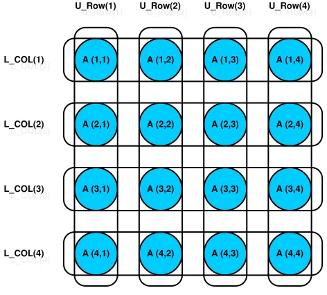
The directive, ALIGN aligns arrays to the templates. We consider an example. The core code of an LU decomposition subroutine looks as follows;
01 REAL A (N, N)
02 INTEGER N, R, R1
03 REAL, DIMENSION (N) :: L_COL, U_ROW
04
05 DO R = 1, N - 1
06 R1 = R + 1
07 L_COL (R : ) = A (R : , R)
08 A (R , R1 : ) = A (R, R1 : ) / L_COL (R)
09 U_ROW (R1 : ) = A (R, R1 : )
10 FORALL (I = R1 : N, J = R1 : N)
11 & A (I, J) = A (I, J) - L_COL (I) * U_ROW (J)
12 ENDDO
After looking through the above algorithm, we can choose a template,
!HPF$ TEMPLATE T (N, N)
The major data structure of the problem, the array A that holds the matrix, is identically matched with this template. In order to align A to T we need an ALIGN directive like;
!HPF$ ALIGN A(I, J) WITH T (I, J)
Here, integer subscripts of “alignee”—the array which is to be aligned—are calledalignment dummies. In this manner, every element of the alignee is mapped to some element of the template.
Most of the work in each iteration of the DO-loop from our example is in the following statement, which is line 11 of the program,
A (I, J) = A (I, J) - L_COL (I) * U_ROW
A (1,1) A (1,2) A (1,3) A (1,4)
A (4,1) A (4,2) A (4,3) A (4,4) A (3,1) A (3,2) A (3,3) A (3,4) A (2,1) A (2,2) A (2,3) A (2,4)
L_COL(1)
L_COL(1)
L_COL(4)
L_COL(4)
L_COL(3)
L_COL(3)
L_COL(2)
L_COL(2)
U_Row(1)
U_Row(1)
U_Row(4)
U_Row(4)
U_Row(3)
U_Row(3)
U_Row(2)
[image:28.595.190.426.121.334.2]U_Row(2)
Figure 2.5. Alignment of the three arrays in the LU decomposition example
!HPF$ ALIGN L_COL (I) WITH T (I, *)
!HPF$ ALIGN U_ROW (J) WITH T (*, I)
where an asterisk means that array elements are replicated in the corresponding processor dimension, i.e. a copy of these elements is shared across processors. Figure 2.5 shows the alignment of the three arrays and the template. Thus, no communications are needed for the assignment in the FORALLconstruct since all operands of each elemental assignment will be allocated on the same processor. Do the other statements require some communications?
The line 8 is equivalent to
FORALL (J = R1 : N) A (R, J) = A (R, J) / L_COL (R)
Since we know that a copy of L_COL (R) will be available on any processor wherever A (R, J) is allocated, it requires no communications.
But, the other two array assignment statements do need communications. For instance, the assignment to L_COL, which is the line 7 of the program, is equivalent to
FORALL (I = R : N) L_COL (I) = A (I, R)
to broadcast the A element to all concerned parties. These communications will be properly inserted by the compiler.
The next step is to distribute the template (we already aligned the arrays to a template). A BLOCK distribution is not good choice for this algorithm since successive iterations work on a shrinking area of the template. Thus, a block distribution will make some processors idle in later iterations. A CYCLIC distribution will accomplish better load balancing
In the above example, we illustrated simple alignment—“identity mapping” array to template—and also replicated alignments. What would general alignments look like?
One example is that we can transpose an array to a template.
DIMENSION B(N, N)
!HPF$ ALIGN B(I, J) WITH T(J, I)
transpositionally mapsBtoT(B (1, 2)is aligned toT (2, 1), and so on). More generally, a subscript of an align target (i.e. the template) can be a linear expression in one of the alignment dummies. For example,
DIMENSION C(N / 2, N / 2)
!HPF$ ALIGN C(I, J) WITH T(N / 2 + I, 2 * J)
The rank of the alignee and the align-target don’t need to be identical. An alignee can have a “collapsed” dimension, an align-target can have “constant” subscript (e.g. a scalar might be aligned to the first element of a one-dimensional template), or an alignee can be “replicated” over some dimensions of the template:
DIMENSION D(N, N, N)
!HPF$ ALIGN D(I, J, K) WITH T(I, J)
2.3
Message-Passing for HPC
2.3.1 Overview and Goals
The message passing paradigm is a generally applicable and efficient programming model for distributed memory parallel computers, that has been widely used for the last decade and an half. Message passing is a different approach from HPF. Rather than designing a new parallel language and its compiler, message passing library routines explicitly let processes communicate through messages on some classes of parallel machines, especially those with distributed memory.
Since there were many message-passing vendors who had their own implementations, a message-passing standard was needed. In 1993, the Message Passing Interface Forum established a standard API for message passing library routines. Researchers attempted to take the most useful features of several implementations, rather than singling out one existing implementation as a standard. The main inspirations of MPI were from PVM [17], Zipcode [44], Express [14], p4 [7], PARMACS [41], and systems sold by IBM, Intel, Meiko Scientific, Cray Research, and nCube.
The major advantages of making a widely-used message passing standard are portability and scalability. In a distributed memory communication environment where the higher level of routines and/or abstractions build on the lower level message passing routines, the benefits of the standard are obvious. The message passing standard lets vendors make efficient message passing implementations, accommodating hardware support of scalability for their platform.
2.3.2 Early Message-Passing Frameworks
monitors. For the distributed-memory machines, p4 supports send, receive, and process creation libraries.
p4 is still used in MPICH [21] for its network implementation. This version of p4 uses Unix sockets in order to execute the actual communication. This strategy allows it to run on a diverse machines.
PARMACS [41] is tightly associated with the p4 system. PARMACS is a collection of macro extensions to the p4 system. In the first place, it was developed to make Fortran interfaces to p4. It evolved into an enhanced package which supported various high level global operations. The macros of PARMACS were generally used in order to configure a set of p4 processes. For example, the macro torus created a configuration file, used by p4, to generate a 3-dimensional graph of a torus. PARMACS influenced the topology features of MPI.
PVM (Parallel Virtual Machine) [17] was produced as a byproduct of an ongoing heterogeneous network computing research project at Oak Ridge National Laboratory in the summer of 1989. The goal of PVM was to probe heterogeneous network computing—one of the first integrated collections of software tools and libraries to enable machines with varied architecture and different floating-point representation to be viewed as a single parallel virtual machine. Using PVM, one could make a set of heterogeneous computers work together for concurrent and parallel computations.
PVM supports various levels of heterogeneity. At the application level, tasks can be executed on best-suited architecture for their result. At the machine level, machines with different data formats are supported. Also, varied serial, vector, and parallel architectures are supported. At the network level, a Parallel Virtual Machine consists of various network types. Thus, PVM enables different serial, parallel, and vector machines to be viewed as one large distributed memory parallel computer.
2.3.3 MPI: A Message-Passing Interface Standard
The main goal of the MPI standard is to define a common standard for writing message passing applications. The standard ought to be practical, portable, efficient, and flexible for message passing. The following is the complete list of goals of MPI [18], stated by the MPI Forum.
• Design an application programming interface (not necessarily for compilers or a system implementation library).
• Allow efficient communication: avoid memory-to-memory copying and allow overlap of com-putation and communication, and offload to communication co-processor, where available.
• Allow for implementations that can be used in a heterogeneous environment.
• Allow convenient C and Fortran 77 bindings for the interface.
• Assume a reliable communication interface: the user need not cope with communication failures. Such failures are dealt with by the underlying communication subsystem.
• Define an interface that is not too different from current practice, such as PVM, NX, Express, p4, etc., and provide extensions that allow greater flexibility.
• Define an interface that can be implemented on many vendor’s platforms, with no significant changes in the underlying communication and system software.
• Semantics of the interface should be language independent.
• The interface should be designed to allow for thread-safety.
The standard covers point-to-point communications, collective operations, process groups, communication contexts, process topologies, bindings for Fortran 77 and C, environmental management and inquiry, and a profiling interface.
The main functionality of MPI, the point-to-point and collective communication of MPI are generally executed within process groups. A group is an ordered set of processes, each process in the group is assigned a unique rank such that 0, 1, . . . ,p−1, wherepis the number of processes. A context is a system-defined object that uniquely identifies a communicator. A message sent in one context can’t be received in other contexts. Thus, the communication context is the fundamental methodology for isolating messages in distinct libraries and the user program from one another.
communication context together into a communicator. A communicator is a data object that specializes the scope of a communication. MPI supports an initial communicator, MPI_COMM_WORLDwhich is predefined and consists of all the processes running when program execution begins.
Point-to-point communication is the basic concept of MPI standard and fundamental for send and receive operations for typed data with associated message tag. Using the point-to point communication, messages can be passed to another process with explicit message tag and implicit communication context. Each process can carry out its own code in MIMD style, sequential or multi-threaded. MPI is made thread-safe by not using global state3.
MPI supports the blocking send and receiveprimitives. Blocking means that the sender buffer can be reused right after the send primitive returns, and the receiver buffer holds the complete message after the receive primitive returns. MPI has one blocking receive primitive, MPI_RECV, but four blocking send primitives associated with four different communication modes: MPI_SEND (Standard mode), MPI_SSEND (Synchronous mode), MPI_RSEND (Ready mode), and MPI_BSEND (Buffered mode).
Moreover, MPI supports non-blocking send and receive primitives including MPI_ISEND and MPI_IRECV, where the message buffer can’t be used until the communication has been completed by a wait operation. A call to a non-blocking send and receive simply posts the communication operation, then it is up to the user program to explicitly complete the communication at some later point in the program. Thus, any non-blocking operation needs a minimum of two function calls: one call to start the operation and another to complete the operation.
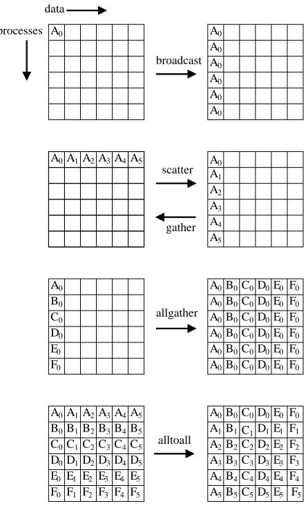
A collective communication is a communication pattern that involves all the processes in a communicator. Consequently, a collective communication is usually associated with more than two processes. A collective function works as if it involves group synchronization. MPI supports the following collective communication functions: MPI_BCAST, MPI_GATHER, MPI_SCATTER, MPI_ALLGATHER, andMPI_ALLTOALL.
Figure 2.6 on page 19 illustrates the above collective communication functions with 6 processes.
3
The MPI specification is thread safe in the sense that it does notrequireglobal state. Particular MPI
0 A 0 A 0 A 0 A 0 A 0
A A1 A0
A1 A2 A2 A3 A3 A4 A4 A5 A5 0 A B0 C0 D0 E0 0 F 0
A B0C0D0E0 F0
0
A B0C0D0E0 F0
0
A B0C0D0E0 F0
0
A B0C0D0E0 F0
0
A B0C0D0E0 F0
0
A B0C0D0E0 F0
0
F F1 F2 F3 F4 F5
E0 E1 E2 E3 E4 E5
D0D1D2D3D4D5
C0C1C2C3C4C5
B0B1B2B3B4B5
A5 A4 A3 A2 A1 0
A A0
A1 A2 A3 A4 A5 B1 B2 B3 B4 B5 C0 C1 C2 C3 C4 C5 D0 D1 D2 D3 D4 D5 E0 E1 E2 E4 E5 1 F 2 F 3 F 4 F 5 F B0 E3 0 F 0
A A0
[image:34.595.197.420.116.484.2]processes scatter gather data allgather alltoall broadcast
Figure 2.6. Collective communications with 6 processes.
A user-defined data type is taken as an argument of all MPI communication functions. The data type can be, in the simple case, a primitive type like integer or floating-point number. As well as the primitive types, a user-defined data type can be the argument, which makes MPI communication powerful. Using user-defined data types, MPI provides for the communication of complicated data structures like array sections.
2.4
High Level Libraries for Distributed Arrays
DO I = 1, N
X(IA(I)) = X(IA(I)) + Y(IB(I)) ENDDO
Figure 2.7. Simple sequential irregular loop.
type. Unlike an ordinary array, the index space and associated elements are scattered across the processes that share the array.
The communication patterns implied by data-parallel languages like HPF can be complex. Moreover, it may be hard for a compiler to create all the low-level MPI calls to carry out these communications. Instead, the compiler may be implemented to exploit higher-level libraries which directly manipulate distributed array data. Like the run-time libraries used for memory management in sequential programming languages, the library that a data parallel compiler uses for managing distributed arrays is often called its run-time library.
2.4.1 PARTI
The PARTI [16] series of libraries was developed at University of Maryland. PARTI was originally designed for irregular scientific computations.
In irregular problems (e.g. PDEs on unstructured meshes, sparse matrix algorithms, etc) a compiler can’t anticipate data access patterns until run-time, since the patterns may depend on the input data, or be multiply indirected in the program. The data access time can be decreased by pre-computing which data elements will be sent and received. PARTI transforms the original sequential loop to two constructs, called the inspector and executor loops.
First, the inspector loop analyzes the data references and calculates what data needs to be fetched and where they should be stored. Second, the executor loop executes the actual computation using the information generated by the inspector.
Figure 2.7 is a basic sequential loop with irregular accesses. A parallel version from [16] is illustrated in Figure 2.8.
C Create required schedules (Inspector):
CALL LOCALIZE(DAD_X, SCHEDULE_IA, IA, LOCAL_IA, I_BLK_COUNT, OFF_PROC_X)
CALL LOCALIZE(DAD_Y, SCHEDULE_IB, IB, LOCAL_IB, I_BLK_COUNT, OFF_PROC_Y)
C Actual computation (Executor):
CALL GATHER(Y(Y_BLK_SIZE + 1), Y, SCHEDULE_IB) CALL ZERO_OUT_BUFFER(X(X_BLK_SIZE + 1), OFF_PROC_X) DO L = 1, I_BLK_COUNT
X(LOCAL_IA(I)) = X(LOCAL_IA(I)) + Y(LOCAL_IA(I)) ENDDO
CALL SCATTER_ADD(X(X_BLK_SIZE + 1), X, SCHEDULE_IA)
Figure 2.8. PARTI code for simple parallel irregular loop.
is returned in SCHEDULE_IA. Setting up the communication schedule involves resolving the requests of accesses, sending lists of accessed elements to the owner processors, detecting proper accumulation and redundancy eliminations, etc. The result is some list of messages that contains the local sources and destinations of the data. Another input argument of LOCALIZE is the descriptor of the data array, DAD_X. The second call works in the similar way with respect to Y(IA(I)).
We have seen the inspector phrase for the loop. The next is the executor phrase where actual computations and communications of data elements occurs.
A collective call, GATHER fetches necessary data elements from Y into the target ghost regions which begins at Y(Y_BLK_SIZE + 1). The argument, SCHEDULE_IB, includes the communication schedule. The next call ZERO_OUT_BUFFER make the value of all elements of the ghost region of X zero.
In the main loop the results for locally owned X(IA)elements are aggregated directly to the local segment X. Moreover, the results from non-locally owned elements are aggregated to the ghost region ofX.
The final call, SCATTER_ADD, sends the values in the ghost region of X to the related owners where the values are added in to the physical region of the segement.
those schedules. The immediate benefit of this separation arises in the common situation where the form of the inner loop is constant over many iterations of some outer loop. The same communication schedule can be reused many times. The inspector phase can be moved out of the main loop. This pattern is supported by the Adlib library used in HPJava.
2.4.2 The Global Array Toolkit
The main issue of the Global Array [35] (GA) programming model is to support a portable interface that allows each process independent, asynchronous, and efficient access to blocks of physically distributed arrays without explicit cooperation with other processes. In this respect, it has some characteristics of shared-memory programming. However, GA encourages data locality since it takes more work by the programmer to access remote data than local data. Thus, GA has some characteristic of message-passing as well.
The GA Toolkit supports some primitive operations that are invoked collectively by all processes: create an array controlling alignment and distribution, destroy an array, and synchronize all processes.
In addition, the GA Toolkit provides other primitive operations that are invoked in MIMD style: fetch, store, atomic accumulate into rectangular patches of a two-dimensional array; gather and scatter; atomic read and increment array element; inquire the location and distribution of data; directly access local elements of array to provide and improve performance of application-specific data parallel operations.
2.4.3 NPAC PCRC Runtime Kernel – Adlib
Adlib supports a built-in representation of a distributed array, and a library of com-munication and arithmetic operations acting on these arrays. The array model supports HPF-like distribution formats, and arbitrary sections, and is more general than GA. The Adlib communication library concentrates on collective communication rather than one-sided communication. It also provides some collective gather/scatter operations for irregular access.
A Distributed Array Descriptor (DAD) played an very important role in earlier imple-mentation of the Adlib library. A DAD object describes the layout of elements of an array distributed across processors. The original Adlib kernel was a C++ library, built on MPI. The array descriptor is implemented as an object of typeDAD. The public interface of theDAD had three fields. An integer value, rank is the dimensionality,r, of the array, greater than or equal to zero. A process group object, group, defines a multidimensional process grid embedded in the set of processes executing the program—the group over which the array is distributed. A vector, maps, has r map objects, one for each dimension of the array. Each map object was made up of an integer local memory stride and arange object.
There are several interfaces to the kernel Adlib. The shpf Fortran interface is a Fortran 90 interface using a kind of dope vector. The PCRC Fortran interface is a Fortran 77 interface using handles to DAD objects. Thead++interface is a high-level C++ interface supporting distributed arrays as template container classes. An early HPJava system used a Java Native Interface (JNI) wrapper to the original C++ version of Adlib.
2.5
Discussion
In this chapter we have given a historical review of data parallel languages, High Performance Fortran (HPF), message-passing systems for HPC, and high-level libraries for distributed arrays.
HPF is an extension of Fortran 90 to support the data parallel programming model on distributed memory parallel computers. Despite of the limited success of HPF, many of the originally defined goals for HPF standardization of a distributed data model for SPMD programming are important and affect contemporary data parallel languages.
Message-passing is a different approach from HPF. It explicitly lets processes commu-nicate through messages on classes of parallel machines with distributed memory. The Message Passing Interface (MPI) established a standard API for message-passing library routines, inspired by PVM, Zipcode, Express, p4, PARMACS, etc. The major advantages making MPI successful are its portability and scalability.
High-level libraries for distributed arrays, such as PARTI, The Global Array Toolkit, and NPAC PCRC Runtime Kernel – Adlib, are designed and implemented in order to avoid low-level, and complicated communication patterns for distributed arrays.
CHAPTER 3
THE HPSPMD PROGRAMMING MODEL
The major goal of the system we are building is to provide a programming model that is a flexible hybrid of HPF-like data-parallel language features and the popular, library-oriented, SPMD style, omitting some basic assumptions of the HPF model. We refer to this model as the HPspmd programming model.
The HPspmd programming model adds a small set of syntax extensions to a base language, which in principle might be (say) Java, Fortran, or C++. The syntax extensions add distributed arrays as language primitives, and a few new control constructs such as on, overall, and at. Moreover, it is necessary to provide bindings from the extended language to various communication and parallel computation libraries.
3.1
Motivations
The SPMD programming style has been popular and successful, and many parallel applications have been written in the most basic SPMD style with direct low-level message-passing such as MPI [18]. Moreover, many high-level parallel programming environments and libraries incorporating the idea of the distributed array, such as the Global Array Toolkit [35], can claim that SPMD programming style is their standard model, and clearly work. Despite the successes, the programming approach lacks the uniformity and elegance of HPF—there is no unifying framework. Compared with HPF, allocating distributed arrays and accessing their local and remote elements are clumsy. Also, the compiler does not provide the safety of compile-time checking.
Our model is an explicitly SPMD programming model supplemented by syntax—for representing multiarrays, for expressing that some computations are localized to some processors, and for constructing a distributed form of the parallel loop. The claim is that these features make calls to various data-parallel libraries (e.g. high level libraries for communications) as convenient as making calls to array intrinsic functions in Fortran 90. We hope that our language model can efficiently handle various practical data-parallel algorithms, besides being a framework for library usage.
3.2
HPspmd Language Extensions
In order to support a flexible hybrid of the data parallel and low-level SPMD approaches, we need HPF-like distributed arrays as language primitives in our model. All accesses to non-local array elements, however will be done via library functions such as calls to a collective communication libraries, or simply get or put functions for access to remote blocks of a distributed array. This explicit communication encourages the programmer to write algorithms that exploit locality, and greatly simplifies the compiler developer’s task.
The HPspmd programming model we discuss here has some similar characteristics to the HPF model. But, the HPF-like semantic equivalence between a data parallel program and a sequential program is given up in favor of a literal equivalence between the data parallel program and an SPMD program. Understanding a SPMD program is obviously more difficult than understanding a sequential program. This means that our language model may be a little bit harder to learn and use than HPF. In contrast, understanding the performance of a program should be easier.
3.3
Integration of High-Level Libraries
Libraries play a most important role in our HPspmd programming model. In a sense, the HPspmd language extensions are simply a framework to make calls to libraries that operate on distributed arrays. Thus, an essential component of our HPspmd programming model is to define a series of bindings of SPMD libraries and environments in HPspmd languages.
Various issues must be mentioned in interfacing to multiple libraries. For instance, low-level communication or scheduling mechanisms used by the different libraries might be incompatible. As a practical matter, these incompatibilities must be mentioned, but the main thrust of own research has been at the level of designing compatible interfaces, rather than solving interference problems in specific implementations.
There are libraries such as ScaLAPACK [4] and PetSc [3] which are similar to standard nu-merical libraries. For example, they support implementations of standard matrix algorithms, but are executed on elements in regularly distributed arrays. We suppose that designing HPspmd interfaces for the libraries will be relatively straightforward. ScaLAPACK, for instance, supports linear algebra library routines for distributed-memory computers. These library routines work on distributed arrays (and matrices, especially). Thus, it should not be difficult to use ScaLAPACK library routines from HPspmd frameworks.
There are also libraries primarily supporting general parallel programming with regular distributed arrays. They concentrate on high-level communication primitives rather than specific numerical algorithms. We reviewed detailed examples in the section 2.4 of the previous chapter.
3.4
The HPJava Language
HPJava [10, 9] is an implementation of our HPspmd programming model. It extends the Java language with some additional syntax and with some pre-defined classes for handling multiarrays. The multiarray model is adopted from the HPF array model. But, the programming model is quite different from HPF. It is one of explicitly cooperating processes. All processes carry out the same program, but the components of data structures are divided across processes. Each process operates on locally held segment of an entire multiarray.
3.4.1 Multiarrays
As mentioned before, Java is an attractive programming language for various reasons. But it needs to be improved for solving large computational tasks. One of the critical Java and JVM issues is the lack oftrue multidimensional arrays1 like those in Fortran, which are arguably the most important data structures for scientific and engineering computing.
Java does not directly provide arrays with rank greater than 1. Instead, Java represents multidimensional arrays as “array of arrays.” The disadvantages of Java multidimensional arrays result from the time consumption for out-of-bounds checking, the ability to alias rows of an array, and the cost of accessing an element. In contrast, accessing an element in Fortran 90 is straightforward and efficient. Moreover, an array section can be implemented efficiently.
HPJava supports a true multidimensional array, called a multiarray, which is a modest extension to the standard Java language. The new arrays allow regular section subscripting, similar to Fortran 90 arrays. The syntax for the HPJava multiarray is a subset of the syntax introduced later for distributedarrays.
The type signature and constructor of the multiarray has double brackets to tell them from ordinary Java arrays.
int [[*,*]] a = new int [[5, 5]] ;
double [[*,*,*]] b = new double [[10, n, 20]] ; int [[*]] c = new int [[100]] ;
int [] d = new int [100] ;
1
J.E. Moreira proposedJava Specification Request for a multiarray package, because, for scientific and
a, b, c are respectively a 2-dimensional integer array, 3-dimensional double array, and 1-dimensional int array. The rank is determined by the number of asterisks in the type signature. The shape of a multiarray is rectangular. Moreover, c is similar in structure to the standard array d. But, c and d are not identical. For instance, c allows section subscripting, but d does not. The value d would not be assignable to c, or vice versa.
Access to individual elements of a multiarray is represented by a subscripting operation involving single brackets, for example,
for(int i = 0 ; i < 4 ; i++) a [i, i + 1] = i + c [i] ;
In the current sequential context, apart from the fact that a single pair of brackets might include several comma-separated subscripts, this kind of subscripting works just like ordinary Java array subscripting. Subscripts always start at zero, in the ordinary Java or C style (there is no Fortran-like lower bound).
Our HPJava imports a Fortran-90-like idea of array regular sections. The syntax for section subscripting is different to the syntax for local subscripting. Double brackets are used. These brackets can include scalar subscripts or subscript triplets. A section is an object in its own right—its type is that of a suitable multi-dimensional array. It describes some subset of the elements of the parent array. For example, in
int [[]] e = a [[2, :]] ;
foo(b [[ : , 0, 1 : 10 : 2]]) ;
e becomes an alias for the 3rd row of elements of a. The procedure foo should expect a two-dimensional array as argument. It can read or write to the set of elements ofb selected by the section. The shorthand : selects the whole of the index range, as in Fortran 90.
3.4.2 Processes
An HPJava program is started concurrently in all members of some process collection2. From HPJava’s point of view, the processes are arranged by special objects representing process groups. In general the processes in an HPJava group are arranged in multidimensional grids.
2
Most time, we will talk aboutprocesses instead ofprocessors. The different processes may be executed
P
Figure 3.1. The process grids illustrated by p
Group
Procs
[image:45.595.227.385.119.252.2]Procs1 Procs2 Procs0
Figure 3.2. The Group hierarchy of HPJava.
Suppose that a program is running concurrently on 6 or more processes. Then, one defines a 2 × 3 process grid by:
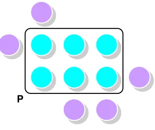
Procs2 p = new Procs2(2, 3) ;
Procs2 is a class describing 2-dimensional grids of processes. Figure 3.1 illustrates the grid p, which assumes that the program was executing in 11 processes. The call to the Procs2 constructor selected 6 of these available processes and incorporated them into a grid.
0
1
2 1
0
e
[image:46.595.215.403.117.265.2]d
Figure 3.3. The process dimension and coordinates in p.
After creating p, we will want to run some code within the process group. The on construct limits control to processes in its parameter group. The code in the onconstruct is only executed by processes that belong to p. The on construct fixes p as the active process group within its body.
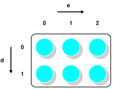
The Dimension class represents a specific dimension or axis of a particular process grid. Called process dimensions, these are available through the inquiry method dim(r), where r is in the range 0, ..., R−1 (R is the rank of the grid). Dimension has a method crd(), which returns the localprocess coordinateassociated with the dimension. Thus, the following HPJava program crudely illustrates the process dimension and coordinates in pfrom Figure 3.3.
Procs2 p = new Procs2(2, 3) ; on (p) {
Dimension d = p.dim(0), e = p.dim(1) ;
System.out.println("(" + d.crd() + ", " + e.crd() + ")") ; }
3.4.3 Distributed Arrays
0 0 2 1 1 p.dim(0)
a[0,3]a[0,4]a[0,5] a[1,3]a[1,4]a[1,5]
a[3,3]a[3,4]a[3,5] a[2,3]a[2,4]a[2,5]
a[4,3]a[4,4]a[4,5] a[5,3]a[5,4]a[5,5]
a[7,3]a[7,4]a[7,5] a[6,3] a[6,5] a[4,0]a[4,1]a[4,2]
a[5,0]a[5,1]a[5,2]
a[7,0]a[7,1]a[7,2] a[6,0]a[6,1]a[6,2]
a[0,6] a[0,7] a[1,6] a[1,7] a[3,6] a[3,7] a[2,6] a[2,7] a[4,6] a[4,7] a[5,6] a[5,7] a[7,6] a[7,7] a[6,6] a[0,0]a[0,1]a[0,2]
a[1,0]a[1,1]a[1,2]
a[3,0]a[3,1]a[3,2] a[2,0]a[2,1]a[2,2]
a[6,7] a[6,4]
p.dim(1)
Figure 3.4. A two-dimensional array distributed over p.
multidimensional index space, and stores a collection of elements of fixed type. Unlike an ordinary array, associates elements are distributed over the processes that share the array.
The type signatures and constructors of distributed arrays are similar to those of sequential multiarrays (see the section 3.4.1). But the distribution of the index space is parameterized by a special class, Range or its subclasses. In the following HPJava program we create a two-dimensional, N×N, array of floating points distributed over the grid p. The distribution of the array, a, for N = 8 is illustrated in Figure 3.4.
Procs2 p = new Procs2(2, 3) ; on (p) {
Range x = new BlockRange(N, p.dim(0)) ; Range y = new BlockRange(N, p.dim(1)) ;
double [[-,-]] a = new double [[x, y]] on p ;
... }
Procs2 p = new Procs2(2, 3) ; on(p) {
Range x = new BlockRange(N, p.dim(0)) ; Range y = new BlockRange(N, p.dim(1)) ;
double [[-,-]] a = new double [[x, y]] on p ; double [[-,-]] b = new double [[x, y]] on p ; double [[-,-]] c = new double [[x, y]] on p ;
... initialize values in ‘a’, ‘b’
overall(i = x for :) overall(j = y for :)
c [i, j] = a [i, j] + b [i, j] ; }
Figure 3.5. A parallel matrix addition.
The type signature of a multiarray is generally represented as
T [[attr0, . . . ,attrR−1]] bras
where R is the rank of the array and each term attrr is either a single hyphen, -, for a
distributed dimension or a single asterisk, *, for a sequential dimension, the term bras is a string of zero or more bracket pairs, []. In principle, T can be any Java type other than an array type. This signature represents the type of a multiarray whose elements have Java type
T bras
If ‘bras’ is non-empty, the elements of the multiarray are (standard Java) arrays.
3.4.4 Parallel Programming and Locations
Theoverallconstruct is another control construct of HPJava. It represents a distributed parallel loop, sharing some characteristics of theforall construct of HPF. Theindex triplet3 of theoverallconstruct represents a lower bound, an upper bound, and a step, all of which are integer expressions, as follows:
overall(i = x for l : u : s)
The step in the triplet may be omitted as follow:
overall(i = x for l : u)
where the default step is 1. The default of the lower bound, l, is 0 and the default of the upper bound,u, isN−1, whereN is the extent of the range before the forkeyword. Thus,
overall(i = x for :)
means “repeat for all elements, i, in the range x” from figure 3.5.
An HPJava range object can be thought of as a collection of abstract locations. From Figure 3.5, the two lines
Range x = new BlockRange(N, p.dim(0)) ; Range y = new BlockRange(N, p.dim(1)) ;
mean that each of the range x and y has N locations. The symboli scoped by theoverall construct is called adistributed index. Its value is alocation, rather an abstract element of a distributed range than an integer value. It is important that with a few exceptions we will mention later, the subscript of a multiarray must be a distributed index, and the location should be an element of the range associated with the array dimension. This restriction is a important feature, ensuring that referenced array elements are locally held.
Figure 3.6 is an attempt to visualize the mapping of locations from x and y. We will write the locations ofxasx[0],x[1], . . . , x[N -1]. Each location is mapped to a particular group of processes. Locationx[1] is mapped to the three processes with coordinates (0,0), (0,1) and (0,2). Location y[4] is mapped to the two processes with coordinates (0,1) and (1,1).
3
y[0] y[1] y[2] y[3] y[4] y[5] y[6] y[7]
x[0]
x[3] x[2] x[1]
x[4]
x[7] x[6] x[5]
(0, 0)
(1, 2) (1, 1)
(1, 0)
(0, 2) (0, 1)
Figure 3.6. Mapping of x and y locations to the grid p.
In addition to the overall construct, there is an at construct in HPJava that defines a distributed index when we want to update or access a single element of a multiarray rather than accessing a whole set of elements in parallel. When we want to update a[1, 4], we can write:
double [[-,-]] a = new double [[x, y]] ;
// a [1, 4] = 19 ; <--- Not allowed since 1 and 4 are not distributed
// indices, therefore, not legal subscripts.
...
at(i = x[1]) at(j = y[4])
a [i, j] = 19 ;
The semantics of the at construct is similar to that of the on construct. It limits control to processes in the collection that hold the given location. Referring again to Figure 3.6, the outer
at(i = x [1])
construct limits execution of its body to processes with coordinates (0,0), (0,1) and (0,2). The inner
at(j = y [4])