Dynamics and structure from molecular beam experiments

FROM

MOLECULAR BEAM EXPERIMENTS

A thesis submitted to

The Australian National University for the degree of Doctor of Philosophy

Peter Frederic Vohralik

March 1986

(ü)

STATEMENT

Except where acknowledgements are made in the text and in the present statement the candidate was responsible for all of the work reported in this thesis.

The spectra reported in Figure 6.2 and Sections 6.5 and 6.6 were measured by Dr G. Fischer and Dr R.E. Miller.

Peter Frederic Vohralik

Come to my arms, my beamish boy! 0 frabjous day! Callooh! Callay!"

Acknowledgements

I wish to thank my supervisor Dr R.O. Watts for his constant encouragement and expert supervision. It was a pleasure working with him.

I would also like to thank Dr R.E. Miller for numerous discussions and many helpful suggestions.

I am grateful to Dr R.W. Crompton and the members of the Electron and Ion Diffusion Unit, the Research School of Physical Sciences, for giving me the opportunity to study at the Australian National University. Thanks also go to the following for their assistance and encouragment during my stay at the Australian National University: Dr J. Reimers, Dr D.F. Coker, Mr G. Bryant, Mr F. Claremont, Dr M.T. Elford, Mr C.V. Boughton and Mr L. Mitchell.

I would like to thank Prof. K. Takayanagi and Prof. M.H. Alexander for providing the results of their calculations prior to publication.

Special thanks go to the technical staff of the Electron and Ion Diffusion Unit and to the members of the Electronics Unit for their valuable support. The assistance of the programmers and operators of the Computer Services Centre is also gratefully acknowledged. For help with the typing of this manuscript I am indebted to Mrs A. Duncanson and Mrs L. Robins.

Financial support from a Commonwealth Postgraduate Reasearch Award is gratefully acknowledged.

I wish to thank all of my friends for their support and encouragement and for making my stay in Canberra a pleasant one.

A b s t r a c t

M o l e c u l a r beam s c a t t e r i n g methods and l a s e r - b o l o m e t e r

s p e c t r o s c o p i c t e c h n i q u e s were used t o i n v e s t i g a t e t h e d yn am ic al b e h a v i o u r

o f a number of a t o m - m o l e c u l e and m o l e c u l e - m o l e c u l e s y s t e m s . E x t e n s i v e

s c a t t e r i n g c a l c u l a t i o n s were c a r r i e d o u t f o r b o t h He-HF and Ar-HF i n o r d e r

t o a s s e s s t h e a b i l i t y o f a v a i l a b l e i n t e r m o l e c u l a r p o t e n t i a l f u n c t i o n s t o

p r e d i c t t h e me asur ed t o t a l s c a t t e r i n g i n t e n s i t i e s . The c o u p l e d s t a t e s

a p p r o x i m a t i o n was us ed t o s t u d y t h e i n e l a s t i c i n t e g r a l and d i f f e r e n t i a l

c r o s s s e c t i o n s f o r t h e s e s y s t e m s . T o t a l d i f f e r e n t i a l c r o s s s e c t i o n s f o r

He-HF s c a t t e r i n g a r e a d e q u a t e l y d e s c r i b e d u s i n g t h e s p h e r i c a l p a r t o f t h e

i n t e r a c t i o n p o t e n t i a l . T hi s i s n o t t h e c a s e f o r Ar-HF, f o r which t h e

a n i s o t r o p i e s i n t h e p o t e n t i a l p l a y a maj or r o l e i n d e t e r m i n i n g t h e

s c a t t e r i n g b e h a v i o u r .

A c o l o u r c e n t r e l a s e r was u s ed i n c o n j u n c t i o n w i t h m o l e c u l a r beam

t e c h n i q u e s t o me as ur e t h e i n f r a r e d s p e c t r a o f s m a l l c l u s t e r s o f a c e t y l e n e ,

m e th y l a c e t y l e n e and e t h y l e n e . By r e c o r d i n g s p e c t r a f o r a wide r a n g e o f

m o l e c u l a r beam c o n d i t i o n s i t was p o s s i b l e t o a s s e s s t h e c o n t r i b u t i o n s t o

t h e o b s e r v e d s p e c t r a from t h e d i f f e r e n t c l u s t e r s i z e s p r e s e n t i n t h e beams.

I n f r a r e d c l u s t e r d i s s o c i a t i o n s p e c t r a were s t u d i e d und er b o t h low

r e s o l u t i o n ( 0 . 4 cm- ^ ) and h i g h r e s o l u t i o n (0.0001 cm- "'). L i f e t i m e s of t h e

i n i t i a l l y e x c i t e d c l u s t e r s d e t e r m i n e d from t h e homogeneous w i d t h s of t h e

i n d i v i d u a l r o v i b r a t i o n a l t r a n s i t i o n s r a n g e from 1 ps f o r e t h y l e n e t o >80 ns

f o r a c e t y l e n e .

A c o m b i n a t i o n o f s p e c t r o s c o p i c and s c a t t e r i n g t e c h n i q u e s was us ed

t o i n v e s t i g a t e t h e t r a n s f e r o f r o t a t i o n a l e n e r g y bet ween HF m o l e c u l e s i n

(vi)

processes which are dipole allowed to first order were found to dominate the observed scattering. A lower bound of 310 was obtained for the j i=0, j 2=1 -*■ j i = 1,3 2=0 cross section.

The work described in this thesis has been reported in several publications:

Miller R.E., Vohrallk P.F. and Watts R.O. (1984), "Sub-Doppler resolution infrared spectroscopy of the acetylene dimer: A direct measurement of the predissociation lifetime", J. Chem. Phys. 80, 5453.

Fischer G., Miller R.E., Vohrallk P.F. and Watts R.O. (1985), "Molecular beam infrared spectra of dimers formed from acetylene, methyl

acetylene, and ethene as a function of source pressure and concentration", J. Chem. Phys. 83_, 1471.

Vohrallk P.F. and Miller R.E. (1985), "Resonant rotational energy transfer in HF", J. Chem. Phys. 83, 1609.

Boughton C.V., Miller R.E., Vohrallk P.F. and Watts R.O. (1986), "The helium-hydrogen fluoride differential scattering cross section", accepted for publication in Molecular Physics.

TABLE OF CONTENTS

STATEMENT (ii)

ACKNOWLEDGEMENTS (iv)

ABSTRACT (v)

TABLE OF CONTENTS (vii)

TABLE AND FIGURE CAPTIONS (xi)

CHAPTER 1 Introduction 1

CHAPTER 2 EXPERIMENTAL TECHNIQUES 6

2.1 The Beam Chamber 7

2.2 Phase Sensitive Detection 9

2.3 The Quadrupole Mass Spectrometer 10

2.M Bolometric Detection 11

2.5 The Colour Centre Laser 15

(a) Low Resolution Scanning 16

(b) High Resolution Scanning 17

(c) Frequency Stabilized Operation 19 2.6 Quantum State Distributions in Molecular Beams 25 2.7 Differential Scattering Cross Section Measurements 27

(viii)

CHAPTER 3 SCATTERING CALCULATIONS 34

3.1 Introduction 35

3.2 Atom-Diatom Scattering 41

3.3 The Spherical Potential Approximation 49 3.^ The Infinite Order Sudden Approximation 50

3.5 The Coupled States Approximation 52

3.6 The Matrix Elements of the Potential 56 3*7 Solution of the Coupled States Equations 58 3.8 On the Comparison Between Theory and Experiment 61

CHAPTER 4 HELIUM-HYDROGEN FLUORIDE SCATTERING CROSS SECTIONS 68

4.1 Introduction 69

4.2 Experimental Results 77

4.3 The He-HF Interaction Potential 79

4.4 A Comparison between the Present Coupled States

Calculations and Previous Close Coupled Results 82 4.5 A Comparison between Coupled States, IOS and

Spherical Potential Calculations 85 4.6 Inelastic Cross Sections within the Coupled

States Approximation 88

4.7 Comparing Theory with Experiment 93

CHAPTER 5 ARGON-HYDROGEN FLUORIDE SCATTERING CROSS SECTIONS 100

5.1 Introduction 101

5.2 Experimental Results 109

5.3 The Ar-HF Interaction Potential 112

5.4 A Comparison between Spherical Potential, Infinite

Order Sudden and Coupled States Calculations 115

5.5 Comparing Theory with Experiment 122

5.6 State-to-state Cross Sections within the Coupled

States Approximation 125

5.7 Partial Integral Cross Sections 130

5.8 Conclusions 136

CHAPTER 6 INFRARED SPECTROSCOPY OF SMALL CLUSTERS OF ACETYLENE,

METHYL ACETYLENE AND ETHYLENE 138

6.1 Introduction 139

6.2 Monomer Spectroscopy 148

6.3 Experimental 150

6.4 Acetylene Clusters 154

6.4.1 Large Clusters of Acetylene 154

6.4.2 High Resolution Spectroscopy of Small Clusters

of Acetylene 158

6.4.3 Pressure Dependence of the Spectra of Small

Acetylene Clusters 166

6.5 Methyl Acetylene Clusters 173

6.6 Ethylene Clusters 176

(x)

CHAPTER 7 RESONANT ROTATIONAL ENERGY TRANSFER IN HF 181

7.1 Introduction 182

7.2 Experimental 189

7.3 Results 194

7.4 Kinetic Model 199

7.5 Analysis and Discussion 202

7.6 Conclusions 212

CHAPTER 8 SUMMARY AND CONCLUSIONS 213

Table 2.1 Operating point parameters for bolometer B corresponding to the I-V characteristics (labelled A through H) shown in Figures 2.7 and 2.8. The data labelled C through H were obtained under conditions similar to those existing when the spectroscopic studies reported in this thesis were carried out and the pressures P are typical 310 K helium beam stagnation pressures corresponding to these data. (Iq,Vq) is the operating point and Sq is the zero frequency responsivity.

Table 2.2 Frequency response characteristics of some of the components of the laser system. FSR = free spectral range and FWHM = full width at half maximum of the response profile.

17b

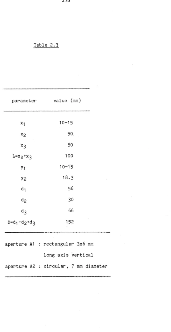
Table 2.3 Parameters describing the geometry of the experimental arrangement used to obtain the total differential scattering cross sections

(see Figure 2.18).

Table 2.4 Parameters of the velocity distributions obtained from the analysis of the measured time-of-flight spectra. Tq is the nozzle temperature; vs and vw are the stream velocity and width parameter; vm p is the most probable velocity of the v3 maxwellian distribution; Av is the FWHM of this distribution;’ T' is the nozzle temperature corresponding to the stream velocity if one assumes an ideal isentropic expansion (see Eqs. (2.13) and (2.14)); and E is the mean kinetic energy of the atoms/molecules in the beam.

32c

(xii)

table are all for beams of pure gases. ' (Boltz)' indicates that the results are for a Boltzmann distribution of velocities. The velocity distributions used for the beams are those given in Table 2.4. Apart from the HF and He(80K) beams, the nozzles used to form the expansions were maintained at 310 K. See the text for more details.

Figure 2.1 A schematic diagram of the crossed molecular beam apparatus. In the elevation view A and B denote the far and near cryostat positions, C is the molecular beam chopper, F is the molecular beam flag, N is the nozzle, S is the skimmer and A.T. is the alignment telescope. In the plan view, B is the bolometer, PBC is the primary beam chamber and SBC is the secondary beam chamber.

7a

Figure 2.2 Details of the nozzle and skimmer geometries. The outside diameter of the nozzle is 1/4". Region A contains the gas of interest at the stagnation pressure Pq and temperature

T

q

.

The supersonic expansion takes place in region B, and region C is the main scattering chamber, a = 60° or 90°; the nozzle diameter d is usually in the range 30-80 pm; the skimmer diameter D is generally between 200 and 600 pm; and B and. Y are 26° and 30° respectively.

7b

Figure 2.3 A schematic diagram of the bolometer cryostat assembly. ]ia

Figure 2.4 The circuit used to operate the bolometer detector. ^

Figure 2.5 The circuit used to measure the I-V characteristics (ie. load curves) of the bolometer.

12b

Figure 2.6 I-V characteristic for bolometer A. (Iq jVq) = (0.69 pA , 5.33 V) is the operating point defined by the load line shown and Va = 3.15 V. The load line is given by V(V) = 8.8 - 5xI(pA).

(xiv)

Laboratories. The operating point defined by the load line shown [ V(V) = 8.8 - 5xI(yA) ] is (1.58 yA , 0.90 V) and the V-intercept of the tangent to the load curve at the operating point is Va = 0.755 V.

a 12d

Figure 2.8 I-V characteristics for bolometer B as a function of the heat flux reaching the bolometer. Curves B and C were measured in the absence of direct molecular beam flux reaching the detector (although the background radiation and molecular fluxes were almost certainly not the same). Characteristics D through H show the changes resulting from increasing the flux of the helium beam used to heat the detector. Also shown are the zero frequency responsivities (in V/mW) at the operating points determined by the load line [ V(V) = 8.8 - 5xI(yA) ]. The operating points are given in Table (2.1).

13a

Figure 2.9 Changes in the output of the bolometer B - LIA detection system (for a small, chopped IR signal of unvarying amplitude) as a function of the helium beam gas load reaching the bolometer.

14a

Figure 2.10 A comparison between the measured response of the bolometer B -LIA detection system and the predicted responsivity of bolometer B obtained from the I-V characteristics as a function of the voltage at the operating point. The shapes of the response profiles are similar,

indicating that, as expected, the overall response of the bolometer-LIA system is determined by the response of the bolometer.

( a d a p t e d from M o l l e n a u e r ( 1 9 8 5 ) ) .

15a

F i g u r e 2 . 1 2 A s c h e m a t i c d i a gr am o f t h e FCL c a v i t y .

16a

F i g u r e 2 . 1 3 An i l l u s t r a t i o n o f t h e f r e q u e n c y r e s p o n s e p r o f i l e s o f t h e FCL

c a v i t y , t h e i n t r a c a v i t y e t a l o n and t h e c a v i t y g r a t i n g . The r e s p o n s e

p r o f i l e s a r e n o t drawn t o t h e same s c a l e .

17a

F i g u r e 2.1-4 The e x p e r i m e n t a l s e t u p u s e d t o o b t a i n h i g h r e s o l u t i o n IR -

m o l e c u l a r beam s p e c t r a w i t h t h e FCL. D1 and D2 a r e IR d e t e c t o r / a m p l i f i e r

u n i t s and LIA1 and LIA2 a r e l o c k - i n a m p l i f i e r s .

18a

F i g u r e 2 . 1 5 E x p e r i m e n t a l a r r a n g e m e n t us ed t o o b t a i n f e e d b a c k s t a b i l i s e d

s i n g l e f r e q u e n c y o p e r a t i o n w i t h t h e FCL. D1 and D2 a r e IR d e t e c t o r

/ a m p l i f i e r u n i t s and LIA1 and LIA2 a r e l o c k - i n a m p l i f i e r s .

20a

F i g u r e 2 . 1 6 Gas c e l l a b s o r p t i o n p r o f i l e s as o b s e r v e d on CR02. 21a

F i g u r e 2 . 1 7 Curves A and B a r e t h e f r e q u e n c y r e s p o n s e p r o f i l e s of t h e 150

MHz e t a l o n t r a n s m i s s i o n s i g n a l a t t h e e x t r e m i t i e s of t h e 600 Hz o s c i l l a t i o n

a p p l i e d t o i t . The l ow er c u r v e i s t h e o u t p u t o f t h e LIA which i s us ed as

t h e f e e d b a c k s i g n a l .

22a

F i g u r e 2 . 1 8 A s c h e m a t i c d i a gr am of t h e e x p e r i m e n t a l a r r a n g e m e n t u sed t o

m e a su r e t o t a l d i f f e r e n t i a l s c a t t e r i n g c r o s s s e c t i o n s . N1 and N2 a r e t h e

n o z z l e s ; S1 , S1 ' and S2 a r e t h e skimmer s; C i s t h e r o t a t i n g s e c o n d a r y beam

(xvi)

bolometer; and A1 and A2 are the apertures in the bolometer cryostat shields. Values of the parameters describing the geometry appear in

Table 2.3. 0-,

27a

Figure 2.19 A schematic diagram of the experimental setup used to obtain the time-of-flight distributions of the molecules in the beams. E is the electron ionization region; A represents the field used to inject the positive ions into the quadrupole region Q; and D is the multi-dynode ion detector.

29a

Figure 2.20 Corrected experimental TOF distributions (dots) for the gases studied. The solid curves are the fitted TOF distributions discussed in the text.

32a

Figure 2.21 v3 maxwellian distributions corresponding to the TOF distributions given in Figure 2.20. They have been normalized to have the same area.

Table 3.1 The equations required to effect the angle transformation from the centre of mass reference frame to the laboratory reference frame.

62a

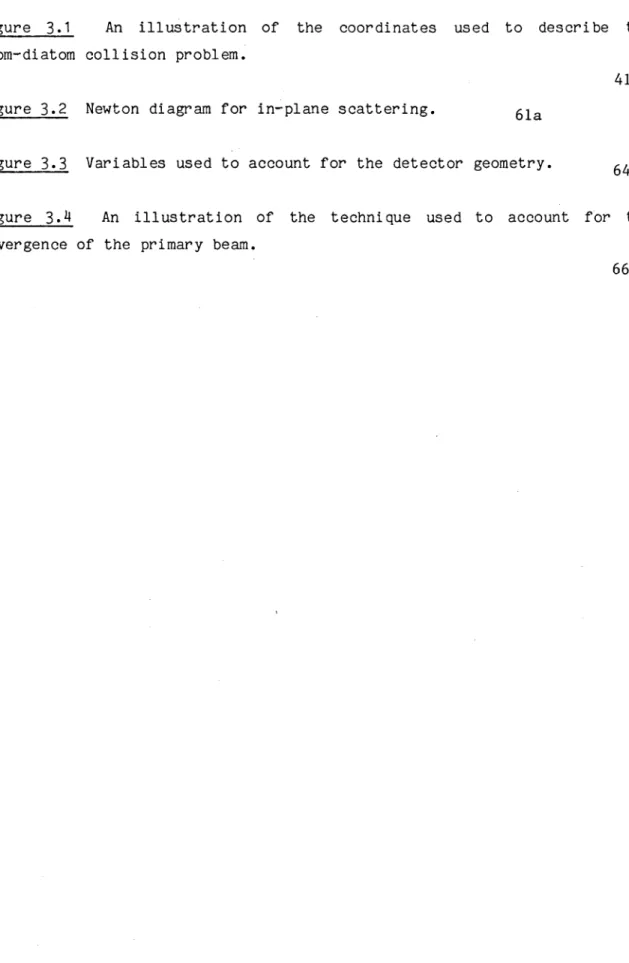
Figure 3.1 An illustration of the coordinates used to describe the atom-diatom collision problem.

41a Figure 3.2 Newton diagram for in-plane scattering. ^

Figure 3.3 Variables used to account for the detector geometry. ^

Figure 3*4 An illustration of the technique used to account for the divergence of the primary beam.

(xviii)

Table 4.1 Measured scattering intensities for the He-HF system as a function of the laboratory scattering angle (in degrees). Results are shown for two mean collision energies corresponding to different primary

(helium) beam conditions. The numbers in parentheses represent two standard deviations in the scatter of values obtained at the corresponding angles. "(-)" indicates that only two measurements were made at the

corresponding angle. y7a

Table 4.2 Experimental conditions used to obtain the differential scattering intensities reported in this chapter. The velocity fitting parameters vs , vw and vm p have estimated uncertainties of ± 0.5 %. These velocity parameters, which were reported in Chapter 2, are duplicated here

for convenience. 7 7k

Table 4.3 Energies (Ej) and asymptotic wavevectors (kj) and wavelengths (Xj) for the basis set used in the CS calculations at a total energy of

313 K.

82a

Table 4.4 Centre of mass frame integral cross sections for He-HF at a total energy of 313 K obtained using the rigid rotor and vibration dependent HFD1 potentials. The close coupled results are those of Battaglia £t al. (1984b). Details of the CS calculations are given in the text. The cross sections are in square Angstroms. 82a

Table 4.5 Total integral cross sections obtained using the CS, IOS, spherical potential (quantum) and spherical potential (WKB) approximations.

Table 4.6 Energies (Ej) and asymptotic wavectors (k j ) and wavelengths (Xj) for the basis sets used in the CS calculations at a collision energy of 480

Table 4.7 Energies (Ej ) and asymptotic wavevectors (k j ) and wavelengths

(Xj) for the basis sets used in the CS calculations at a collision energy of 950 K.

88d

Table 4.8 (a) Centre of mass frame integral cross sections for He-HF scattering obtained using the vibration dependent HFD1 potential and the CS approximation for a collision energy of 480 K. The cross sections are in square Ängstroms.

(b) The results in this table were obtained by multiplying the cross sections shown in Table 4.8a by the populations of their initial j states in the HF beam. They are expressed as percentages of the total population weighted cross section.

Oya

Table 4.9 (a) and (b) As for Table 4.8a, except these results are for a collision energy of 950 K.

o9b

rotational state poopulations. _90a

Table 4.11 Properties of the spherical terms of the potential surfaces used to analyse the experimental He-HF scattering data. a is the value of r for which V(r)=0, rm is the position of the minimum in the potential, e is the well depth and Ari is the width of the attractive part of the potential at half its maximum depth. S(51

6

) and S(990) are the fitting parameters, defined by Eq. (3.72) at the two experimental collision energies. The smaller the value of S, the better the fit.

BFW is the Barker potential discussed in the text.

HFD2-A is the HFD2 model with the spherical C

5

term increased by 24 %.

HFD2-B is the HFD2 model with the spherical C

5

term increased by 1

8

% and all other dispersion coefficients recalculated using the method discussed by Rodwell et al. (1982).

HFD1-A is the HFD1 model with the spherical C

5

term increased by 18 %.

HFD-p is the HFD1 model with the value of p (see Eq. (4.4)) increased

Table 4.12 Parameters of the Barker potential (BFW) used to represent the spherical part of the He-HF interaction.

Figure 4.1 He-Ar total differential scattering cross section. Experimental points are represented as diamonds and the solid curve is calculated using the potential of Aziz et al. (1979). The value of the fitting parameter S given by Eq. (3.72) is 2.8x10"3. 7ga

Figure 4.2 Cross sections through the HFD1 potential reported by Rodwell et al. (1982) for different values of the potential angle. These cross sections are for the full potential, which depends upon the HF separation. The HF bond length was fixed at its equilibrium value. 8n

Figure 4.3 A comparison between the close coupled results of Battaglia et a l . (1984b) and the present CS results for He-HF scattering at a total energy of 313 K. The CC results ( - - - ) are for the rigid rotor HFD1 potential. The CS cross sections (--- ) for the same potential appear on the left half of the figure and those for the vibration dependent

HFD1 potential are shown on the right. g2^

Figure 4.4 Total differential scattering cross sections for He~HF predicted by the HFD1 potential using the CS method (--- ), the IOS approximation (... ), an exact single channel calculation with the spherical part of the potential — --- -- — ) and a single channel WKB computation with the same spherical potential (— — — — ). ^

(xxii)

Figure 4.6 The Newton diagram for the collision geometry used in the CS calculations at a kinetic energy of 480 K. See the text for details. gga

Figure 4.7 The Newton diagram for the collision geometry used in the CS calculations at a kinetic energy of 950 K. See the text for details. ggg

Figure 4.8 Population weighted differential scattering cross sections calculated from the full HFD1 potential using the CS method at collision energies corresponding to the mean experimental energies. Notice that whereas Figure 4.3 shows cross sections calculated at the same total energy, in this figure the collision energies are fixed. No averaging over experimental parameters has been done. See the text for details. ggc

Figure 4.9 A comparison between the experimental total differential cross sections (diamonds) and those obtained from a number of different potential surfaces using spherical potential approximation and semiclassical

techniques. gga

Table 5.1 Measured scattering intensities for the Ar-HF system as a function of the laboratory scattering angle (in degrees). Estimates of the uncertainties associated with the reported intensities are given for a few of the scattering angles. See the text for a discussion of these estimates. The experimental conditions are summarised in Table 5.2.

109a

Table 5.2 Experimental conditions used to obtain the differential scattering intensities reported in Table 5.1. The velocity fitting parameters vs , v w and vm p have estimated uncertainties of ± 0.5 %. These velocity parameters, which were reported in Chapter 2, are duplicated here

for convenience. 109b

Table 5.3 Equations and parameters defining the M5 potential. 112a

Table 5.M Energies CEj) and asymptotic wavevectors (kj ) and wavelengths (Aj) for the basis set used in the coupled states calculations. 116a

Table 5.5 Total integral cross sections computed using the spherical potential, infinite order sudden and coupled states approximations. The coupled states results were obtained summing the population weighted state-to-state cross sections. Upper figures were obtained by summing values of 1 from 0 to 220. The lower values were determined by summing

values of 1 from 0 to 300. 117e

(xxiv)

table and summing these weighted values one obtains the corresponding IOS

integral cross sections. 119a

Figure 5.1 Typical classical trajectories in the centre-of-mass frame for the scattering resulting from an interaction with a strong attractive part. The circle gives an indication of the size of the repulsive core of the

potential. 101a

Figure 5.2 Sections of the ArHF-HFD1 potential for fixed values of the potential angle. Note that the vertical scale is logarithmic for energies greater than 50 K. The dashed curve is the spherical average of the

interaction potential. u

Figure 5.3 The same as Figure 5.2, except for the ArHF-HFD2 potential. 112c

Figure 5.^ The same as Figure 5.2, except for the M5 potential. 112d

Figure 5.5 The Newton diagram for the collision geometry used in the coupled states and some of the other calculations. The final velocity vectors for the 0+1 and 1+0 transitions terminate on the labelled corves.

117a

Figure 5.6 A comparison between the total differential scattering intensities calculated using the spherical potential (— — — ), infinite order sudden (— — — ) and coupled states (---) approximations. These results were obtained from Eq. (3.59) (in Ä2 per steradian), and have been multiplied by sinS.S1^ . They have also been smoothed out using a 2 degree angular window to damp the diffraction oscillations. The coupled states state-to-state cross sections were weighted by the populations of the initial rotational states and added to give the results shown in the figure.

(xxvi)

Figure 5.7 As for Figure 5.6, except for the ArHF-HFD2 potential. H 7C

Figure 5.8 The same as Figure 5.6, except for the M5 potential. 117d

Figure 5.9 In this figure we show the total population weighted differential cross section for the ArHF-HFD2 potential obtained using the coupled states approximation. The results in the upper half of the figure have been multiplied by

sin0.0]4//3>

and those in the lower half have not. Neither of the cross sections were angle averaged in order to smooth out the diffraction oscillations.

118a

Figure 5.10 The partial IOS cross sections are shown, as a function of the potential angle Y, for the three potentials considered in this study. These integral cross sections were obtained from JWKB and Born phase shifts for the (spherical) potentials determined from the full potentials by

fixing the potential angle. 119b

calculations, which differ slightly from the most probable experimentally

determined velocities. 122a

Figure 5.12 A comparison between the population weighted coupled states cross sections for the ArHF-HFD1 (— — — ), ArHF-HFD2 (— — — ) and M5 (--- ) potentials and the experimentally determined scattering intensities (diamonds). The uncertainties associated with experimental points for angles less than 10 degrees are smaller than the diamonds. Error bars corresponding to the estimated uncertainties (given in Table 5.1 and discussed in the text) are shown to scale in the lower part of the

diagram at a number of angles. 123a

Figure 5.13 As for Figure 5.12, except this time the factor sinB.S1^ was not used to weight the scattered intensities. 123b

Figure 5.14 Inelastic state-to-state differential scattering cross sections for the ArHF-HFD1 potential calculated using the coupled states approximation. They have been weighted by the measured HF rotational populations, multiplied by

sin0.0^//3>

and angle averaged using a two degree window. The three solid curves (from top to bottom) are the total cross section, the sum of the elastic cross sections, and the sum of the inelastic cross sections. The dashed curves, in order of increasing dash length, correspond to the C M , 1+0, 1+2, 0+2 and 2+3 transitions. 125a

Figure 5.15 As for Figure 5.14, except for the ArHF-HFD2 potential. 125b

(xxviii)

Figure 5.17 This is Figure 5.16 without the s i n 0 . 0 ^ 3 weighting. 125d

Figure 5.18 Total scattering cross sections for initial HF rotational states j =0,1,2 and 3 calculated using the coupled states approximation for the ArHF-HFD1 potential. The four pairs of solid curves (from top to bottom) are the total j+$J' and elastic j+j cross sections for j =0,1,2 and 3 respectively. Results have been population weighted, averaged using a 2 degree window and multiplied by sine.e1^ . The 0+0 and 0+£j ’ curves have been moved up half a decade for clarity. The un-shifted 0+£j ’ cross section is also shown (the dashed curve) so that its magnitude can be compared with the other population weighted results. 126a

Figure 5.19 The same as Figure 5.18, except this time for the ArHF-HFD2

potential. 126b

Figure 5.20 As for Figure 5.18, except for the M5 potential. 126c

F i g u r e 5 . 2 2 As f o r F i g u r e 5 . 2 1 , e x c e p t f o r t h e ArHF-HFD2 p o t e n t i a l . ^ Q b

F i g u r e 5 . 2 3 The same as F i g u r e 5 . 2 1 , b u t t h i s t i me f o r t h e M5 p o t e n t i a l . 130c

F i g u r e 5 . 2 4 In t h e l ow er h a l f of t h i s f i g u r e a r e shown t h e o p a c i t i e s

c a l c u l a t e d u s i n g t h e s p h e r i c a l p o t e n t i a l a p p r o x i m a t i o n f o r t h e ArHF-HFD2

p o t e n t i a l . The c o l l i s i o n s p e e d s us ed a r e t h o s e which were used f o r t h e

c o u p l e d s t a t e s c a l c u l a t i o n s . D i f f e r e n t i a l c r o s s s e c t i o n s o b t a i n e d by

summing v a l u e s o f 1 from 0 t o 85, 110 and 300 a p p e a r i n t h e upper h a l f of

t h e f i g u r e . See t h e t e x t f o r more d e t a i l s . 132a

F i g u r e 5 . 2 5 O p a c i t y f u n c t i o n s f o r t h e ArHF-HFD2 i n t e g r a l c r o s s s e c t i o n s

g i v e n i n T a b l e 5 . 6 . Cur ves l a b e l l e d ( a ) t h r o u g h (h) c o r r e s p o n d t o

p o t e n t i a l a n g l e s of 8 4 . 5 , 7 3 . 6 , 6 3 . 3 , 5 1 . 8 , 4 1 . 0 , 3 0 . 0 , 19.1 and 8 . 5

d e g r e e s r e s p e c t i v e l y .

(x xx )

T ab l e 6.1 Monomer t r a n s i t i o n s f o r a c e t y l e n e , m e th yl a c e t y l e n e and e t h y l e n e

i n t h e r a n g e 3000 t o 3300 cm--' . The c e n t r e f r e q u e n c i e s of t h e c l u s t e r

a b s o r p t i o n s f o r e t h y l e n e a r e t a k e n from F i s c h e r _et a l . ( 1 9 8 3 ) . Those f o r

m e t hy l a c e t y l e n e a r e from F i g u r e s 6 . 1 8 and 6 . 1 9 o f t h i s t h e s i s . The

f r e q u e n c i e s of t h e a c e t y l e n e c l u s t e r bands a r e g iv e n i n T a b l e 6 . 2 .

" i n a c t i v e " d e n o t e s t h a t t h e band i s i n f r a r e d i n a c t i v e i n t h e monomer. The

monomer d a t a a r e t a k e n from t h e p ap er by F i s c h e r e t a l . (1983) and t h e

t a b l e s o f Shimanouchi ( 1 9 7 2 ) . 148a

Ta bl e 6 . 2 A summary o f t h e f u l l w i d t h s a t h a l f maximum of t h e homogeneous

components of t h e i n d i v i d u a l r o v i b r a t i o n a l t r a n s i t i o n s o b s e r v e d i n each o f

t h e s i x c l u s t e r d i s s o c i a t i o n bands of a c e t y l e n e . The r e s u l t s were o b t a i n e d

by c o n v o l u t i n g t h e monomer l i n e s h a p e s w i t h L o r e n t z i a n s t o f i t t h e c l u s t e r

a b s o r p t i o n p r o f i l e s . 165b

T a b l e 6 . 3 The s l o p e s of t h e l o g ( s i g n a l ) vs l o g ( s o u r c e p r e s s u r e ) p l o t s f o r

t h e i n t e n s i t i e s of t h e i n f r a r e d s i g n a l s o b s e r v e d f o r t h e low r e s o l u t i o n

a c e t y l e n e c l u s t e r s p e c t r a shown i n F i g u r e 6 . 1 3 . C l u s t e r s i z e s s u g g e s t e d by

Figure 6.1 A schematic of the beam apparatus showing the position of the multipass mirrors and the bolometer as used to measure the infrared spectra reported in this chapter. See the caption to Figure 2.1.

151a

Figure 6.2 A series of low resolution predissociation spectra obtained for an 11% mixture of acetylene in helium measured using bolometer A. Spectra are plotted in arbitrary units with a positive signal representing a decrease in the energy of the molecular beam. The source pressures used (in kP a ) were: A 480, B 685, C 800, D 915, E 1100, F 1240, G 1490, H 1680, and I 1890. The arrows labelled A and B are the positions of the Fermi shifted monomer absorptions for the V

2

+vi|*'+V

5

^ and V

3

bands of acetylene respectively. The arrow marked SOLID indicates the absorption frequency of solid acetylene (Bottger and Eggers (1964)). 154a

Figure

6.3

Log(signal) vs log(source pressure) plots of the mass signals seen near the acetylene monomer, dimer and trimer masses for beams formed from a mixture of acetylene in helium. The symbols represent the experimental points. Lines of best fit are also shown. Slopes of the lines of best fit are 0.5, 2.4 and 6.0 respectively. See the text for more

details. ' 155a

Figure 6.4 Log(signal) vs log(pressure) plots for the three mass peaks seen near the dimer mass for the 11% acetylene in helium mixture. Slopes of the lines of best fit are 1.5, 1.7 and 4.2 for the mass peaks observed

(xxxii)

Figure 6.5 The concentration and source pressure dependence of the low resolution spectrum of acetylene clusters. The upper spectra were measured using bolometer A. Bolometer B was used to record the lowest scan. Note that the top scan is that spectrum labelled A in Figure 6.2. Under the conditions used to obtain these spectra the dimer, and possibly trimer,

were the only clusters present. 156b

Figure 6.6 The concentration and source pressure dependence of the low resolution spectrum of acetylene clusters measured using bolometer B. See

the text for more details. 157a

Figure 6.7 A low resolution spectrum of a \% acetylene in helium mixture at a source pressure of 1160 kPa. High resolution (single mode) scans from each band are shown as inserts with the frequency scales expanded by a factor of 155. A series of etalon transmission peaks separated by 150 MHz and a monomer absorption, plotted using the same frequency scale as the other inserts, are shown in insert G. All the high resolution scans were obtained using multiple near orthogonal laser - molecular beam crossings. The spectra are plotted so that a laser induced decrease in the molecular beam energy is seen as an upward going transition. 158a

Figure 6.8 A composite high resolution scan of about 0.4 cm“ 1 from acetylene cluster band D. The downward going spikes are attributed to monomer absorptions. Eleven single high resolution scans were required to piece together this portion of the spectrum of band D. The upper trace shows frequency markers separated by 150 MHz. Wavelength increases from

Figure 6.9 An example of the convolution technique used to obtain the homogeneous broadening component of the cluster absorption lineshapes. Two Gaussians were used to fit the Doppler broadened monomer lineshape shown. The fitted monomer profile was then convoluted with a Lorentzian to obtain the fit to the cluster absorption, shown as the upper trace. Solid curves represent the experimental data and broken curves are the fitted lineshapes. The results were obtained using multiple near orthogonal laser

- molecular beam crossings. 165a

Figure 6.10 Monomer and dimer spectra obtained using a single orthogonal laser - molecular beam crossing. The full width at half maximum of the

monomer transition is 4 MHz. 166a

Figure 6.11 A mass spectrum of the \% acetylene in helium mixture obtained at a source pressure of 1100 kPa. The energy of the ionizing electrons was set at 30 eV. The mass scale shown corresponds to the mass readout of the

mass spectrometer. 167a

Figure 6.12 Source pressure dependence of the mass peaks shown in Figure 6.11. The slopes of these curves at the low pressure limit are 0.83, 2.8, 2.8 and 4.35 for the mass 25, 49, 50 and 51 signals respectively.

ID /D

Figure 6.13 Source pressure dependence of the low resolution spectrum of the ]% acetylene in helium mixture. The vertical scales for the individual

(xxxiv)

Figure 6.14 Log(signal) vs log(pressure) data for the intensities of the cluster absorption bands shown in Figure 6.13. In this figure the experimental data have been joined by straight line segments. 169a

Figure 6.15 As for Figure 6.14, except this figure gives the best least squares linear fits to the data. For bands A and B the lowest pressure

datum was not used in the fit. 169b

Figure 6.16 Low resolution spectra for a 2.5$ methyl acetylene in helium mixture at various source pressures.

173a

Figure 6.17 Low resolution spectra for a 1$ methyl acetylene in helium mixture at various source pressures. Note the change in the frequency scale from Figure 6.16. At the lowest pressure the dimer, and possibly trimer, would have been the only clusters present. 1 7 U

Figure 6.18 A low resolution infrared spectrum of small methyl acetylene clusters near 3300 cm-1 . Note the change in the frequency scale from

Figure 6.17. 174a

Figure 6.19 A single mode scan of a portion of band A2 of the methyl acetylene spectrum. The frequency scale was calibrated using a 150 MHz free spectral range confocal etalon. The experimental points are shown as dots. The solid curve is a best least squares fit to the data using three

(xxxvi)

Table 7.1 Parameters describing various beam-beam and beam-gas collisions. HF(beam) refers to a pure HF secondary beam supersonic expansion at a nozzle temperature of about 500 K. HF(boltz) denotes a gaseous sample of HF at a temperature of 300 K. He, HF/He, and HF/Ar refer to supersonic expansions of pure He, \% HF in He and 2% HF in Ar at nozzle temperatures of 310 K. The characteristics of the supersonic expansions have been given in Chapter 2. In this table y is the reduced mass, V is the mean collision speed, vrms is the root mean square speed and E is the mean collision

energy. 192a

Table 1.2 Rotational state distributions are given for a Boltzmann distribution of HF at 300 K, for the secondary beam supersonic expansion of pure HF, and for the various primary beam supersonic expansions of 1 % HF in helium. All populations are expressed as percentages. The upper figures for the primary beam data were obtained with the secondary beam operating at the largest nozzle-skimmer separation. The lower numbers, in parentheses, were determined by extrapolating the attenuation data to zero attenuation, and are therefore estimates of the primary beam populations in the absence of scatterers. A room temperature pyroelectric detector was used to obtain the secondary beam populations.

Table 7.3 Cross sections fitted to each of the four sets of data corresponding to different primary beam source pressures. In this case the ratios of the first order cross sections were determined by Eq. (7.9) and the second order ones were assumed to be equal. The labels A,B,C and D refer to primary beam pressures of 2170,1480,655 and 310 kPa respectively.

Table 7.^ The same as Table 7.3, except this time the second order cross sections were also scaled according to Eq. (7.9). 205a

Table 7.5 Best fit cross sections determined by simultaneously fitting to all four sets of data. The two sets of results correspond to choosing the second order cross sections to be equal or scaling them according to Eq. (7.9). In both cases the ratios of first order cross sections were determined by Eq. (7.9). £ is the sum of square relative deviations, which can be compared with the £'s in Table 7.6. 205b

Table 7.6 Best fit cross sections obtained by fixing the size of the second order cross sections and allowing the first order ones to vary independently. In each case, the second order cross sections were chosen to be equal and the 34-^3 cross section was made equal to the 23+32 cross section. The fitting was performed simultaneously to all four sets of data. £ is the sum of square relative deviations for the best fit in each case.

(xxxviii)

Figure 7.1 A schematic diagram of the experimental arrangement. ^

Figure 7.2 Secondary beam angular profiles for various nozzle-skimmer separations as recorded with the mass spectrometer. A pure argon supersonic expansion at a source pressure of about 175 kPa and a nozzle temperature of 310 K was used. The nozzle diameter was 70 ym. Curves 1 through 5 are in order of decreasing nozzle-skimmer separation. At the nozzle-skimmer separation corresponding to curve 5, the attenuation of the primary beam HF was about 15$ (relative to the secondary beam not operating) for the case of an HF (rather than argon) secondary beam.

191a

Figure 7.3 Plots of ln[(2j + 1 )Pq/Pj ] vs j(j+1) for the secondary HF beam and the four primary beams. The primary beam populations extrapolated to zero attenuation were used. SB labels the secondary beam data and A,B,C and D are the four sets of primary beams data, labelled as in Table 7.2.

194b Figure 7.4 Attenuation curves for the j=0,1,2 and 3 states obtained at the primary beam source pressures shown in Table 7.2. The sets of curves labelled A through D correspond to source pressures of 2170,1480,655 and 310 kPa respectively. The experimental points are shown as diamonds. The solid lines represent the fit to the experimental data obtained using the best fit cross sections given in Table 7.5 for the case in which the second order cross sections were scaled according to Eq. (7.9). The straight lines drawn for j=0 and 1 show the behaviour expected when all of the rotational transfer cross sections are zero. Populations are expressed as percentages of the total primary beam HF population at zero attenuation

(a = 0 ).

Figure 7.5 Plots of the summed rotational state populations, £Pj(a), as a function of a for the four primary beam pressures. 197a

Figure 7.6 Results obtained for j=0,1 and 2 when an argon secondary beam was used. The primary beam source pressure was 930 kPa. 197b

Figure 7.7 A comparison between fits to the j=3 population curve at a primary beam pressure of 1480 kPa obtained using different magnitudes of the second order resonant cross sections. The curves labelled 1,2,4,6 and 7 correspond to the similarly labelled cross sections listed in Table 7.6

1

Chapter One

Introduction

The use of supersonic expansions to form intense beams of neutral atoms and/or molecules was first reported by Kantrowitz and Grey (1951) and Kistiakowsky and Slichter (1951). High intensities in the forward direction and narrow velocity distributions result from the hydrodynamic flow of gas through a suitable opening into a sufficiently high vaccuum. To achieve hydrodynamic flow, the mean free path of the gas on the upstream side of the opening must be smaller than the size of the opening. The properties of beams formed from supersonic expansions are well understood. See, for example, the investigations by Anderson and Fenn (1965), Toennies and Winkelmann (1977), Beijerinck and Verster (1981) and Engelhardt e_t a l .

(1985).

Buck and Pauly (1971), Pack et_ _al. (1982a, 1 982b)). In many cases the dependence of the scattering upon the initial and/or final states of the collision partners can be resolved. If one uses small amounts of the molecules of interest seeded in a light carrier gas, say helium or hydrogen, one can obtain supersonic beams in which the molecules of interest have very low effective temperatures (less than 10 K). Such beams are ideal for carrying out spectroscopic investigations of the molecules, or clusters of molecules (van der Waals clusters), present in the beam

(Travis et al. (1977), Gough et al. (1977), Levy (1981), Janda (1985)). The combination of continuously tunable narrow bandwidth lasers and highly sensitive molecular beam techniques allow the measurement of high resolution spectra free from the effects of Doppler broadening (Gough et a l . (1977), Bernstein (1982)). From spectra of this kind one can often obtain information about the dynamical processes occuring in the systems being studied.

3

information about inelastic scattering via time-of-flight techniques (Serri et al. (1980), Bergmann _et al. (1980)). These methods can also be used to record detailed spectroscopic information about the species present in a given molecular beam. By intersecting the molecular beam with a suitable source of laser radiation prior to bolometric detection one is able to measure the laser-induced change in the molecular beam energy as a function of the laser frequency (Gough

et

a l . (1977,1983), Boughton et al. (1982)). The high sensitivity of bolometer detectors makes them ideal for measuring the spectra of the molecules and van der Waals clusters present in a given molecular beam (Miller (1980)). Mass spectrometry and laser-induced fluorescence detection have also been used to monitor molecular beams which have been excited by suitable laser radiation (Brinza et al. (1983,1984), Vernon _et al. (1982b), Liu et a l . (1984), Page £t al. (1984), Hoffbauer et al. (1983b,1983c), Haynam _et al. (1983), Smalley £t al. (1978)). By combining state-selective methods (such as laser excitation, electrostatic quadrupole state selection, or the time-of-flight methods noted above) with molecular beam scattering techniques, it is possible to investigate both integral and differential scattering cross sections as functions of the initial and/or final states of the collision partners (Barnes et. al. (1982), Borkenhagen et al . (1979), Bergmann e_t a l . (1980), Andres et. a l . (1980), Buck et al. (1984), Wilcomb and Dagdigian (1977), Dagdigian et a l . (1979)).

potentials as accurately as possible, and (2) to understand the dynamical processes involved. Both the complexity of the molecules and the nature of the dynamical processes being investigated will determine the amount of information which can be obtained from studies of this kind.

Detailed experimental and computational studies of the dynamical behaviour of a number of small atom-molecule and molecule-molecule systems are reported in this thesis. Both molecular beam scattering methods and infrared laser spectroscopic techniques were used in combination with bolometric detection during the course of these investigations. The experimental techniques are described in Chapter 2. In Chapter 3 are described both the approximations used to calculate the cross sections reported in this thesis and the method used to compare these cross sections with the measured differential scattering intensities. The results of the research are described and discussed in Chapters 4, 5, 6 and 7. Each of these chapters includes an introduction to the topics discussed therein. An outline of the work reported in these chapters is given below.

The results of a computational study of the scattering of helium from hydrogen fluoride are discussed in Chapter 4. Total differential cross sections predicted using the single channel, infinite order sudden and coupled states approximations are compared with each other and with the available experimental data (Boughton (1986)) for a number of model potentials. An analytic, spherically symmetric potential function is determined by fitting to the measured intensities. Coupled states calculations of the inelastic cross sections are reported for the ab initio potential developed by Rodwell et al. (1981).

5

from h ydr ogen f l u o r i d e i s r e p o r t e d i n C h a p t e r 5. D e t a i l e d s c a t t e r i n g

c a l c u l a t i o n s were c a r r i e d o u t u s i n g t h e s i n g l e c h a n n e l , i n f i n i t e o r d e r

sud den and c o u p l e d s t a t e s a p p r o x i m a t i o n s f o r t h e Ar-HF i n t e r a c t i o n

p o t e n t i a l s d e v e l o p e d by H ut son and Howard (1982b) and D o u k e t i s e_t a l .

( 1 9 8 4 ) . The c a l c u l a t e d c r o s s s e c t i o n s a r e compared w i t h t h e me asur ed

d i f f e r e n t i a l s c a t t e r i n g i n t e n s i t i e s and w i t h p r e v i o u s l y r e p o r t e d i n t e g r a l

c r o s s s e c t i o n s ( Bar nes e t a l . ( 1 9 8 2 ) ) .

The r e s u l t s of an i n f r a r e d l a s e r - m o l e c u l a r beam s p e c t r o s c o p i c

i n v e s t i g a t i o n o f s m a l l c l u s t e r s of a c e t y l e n e , e t h y l e n e and m e th yl a c e t y l e n e

a r e p r e s e n t e d i n C h a p t e r 6. A c o n t i n u o u s l y t u n a b l e c o l o u r c e n t r e l a s e r was

u s e d t o me asur e c l u s t e r d i s s o c i a t i o n s p e c t r a under b o t h h i g h ( 0 . 4 cm“ ^ ) and

low (0.0001 cm- 1) r e s o l u t i o n i n t h e v i c i n i t y o f 3000 cm“ ^ . A d i s c u s s i o n o f

t h e p o s s i b l e s t r u c t u r a l and d yn a m i c a l i m p l i c a t i o n s of t h e me asu re d s p e c t r a

i s g i v e n .

An e x p e r i m e n t a l s t u d y o f t h e r e s o n a n t t r a n s f e r of r o t a t i o n a l

e n e r g y between HF m o l e c u l e s i s r e p o r t e d i n C h a p t e r 7. By c ombining

m o l e c u l a r beam s c a t t e r i n g methods and i n f r a r e d l a s e r s p e c t r o s c o p i c

t e c h n i q u e s i t was p o s s i b l e t o e s t i m a t e t h e m a g n i t u d e s of t h e r e s o n a n t

t r a n s f e r c r o s s s e c t i o n s . These c r o s s s e c t i o n s c o r r e s p o n d t o p r o c e s s e s i n

which t h e c o l l i d i n g HF m o l e c u l e s exchange t h e i r r o t a t i o n a l quantum numbers ,

and a r e d e t e r m i n e d p r i m a r i l y by t h e l o n g r a n g e d i p o l e - d i p o l e i n t e r a c t i o n .

F i n a l l y , a summary o f t h e r e s u l t s r e p o r t e d i n t h i s t h e s i s and t h e

C h a p t e r Two

E x p e r i m e n t a l T e c h n i q u e s

In t h i s c h a p t e r we d e s c r i b e t h e e qu ipmen t and t e c h n i q u e s us ed t o

o b t a i n t h e e x p e r i m e n t a l r e s u l t s p r e s e n t e d i n t h i s t h e s i s . The f o l l o w i n g

t o p i c s a r e d i s c u s s e d : t h e beam chamber, p ha s e s e n s i t i v e d e t e c t i o n , t h e

q u a d r u p o l e mass s p e c t r o m e t e r , t h e b o l o m e t e r d e t e c t i o n s y s t e m , t h e c o l o u r

c e n t r e i n f r a r e d l a s e r and a s s o c i a t e d s p e c t r o s c o p i c t e c h n i q u e s , t h e

me asur ement of a t o t a l d i f f e r e n t i a l s c a t t e r i n g c r o s s s e c t i o n and t h e

t i m e - o f - f l i g h t d e t e r m i n a t i o n o f t h e v e l o c i t y d i s t r i b u t i o n o f t h e m o l e c u l e s

7

2.1 The Beam Chamber

The molecular beam system used in the present investigations has been described by Boughton et al. (1982) and Hiller et al. (1984a). A schematic diagram of the apparatus is shown in Figure 2.1. It consists of a stainless steel chamber and a rotatable base flange between which a conventional O-ring seal is located. Mounted on the base flange are the primary and secondary supersonic molecular beam source chambers which are pumped by an unbaffled 5300 1/s and an unbaffled 2400 1/s oil diffusion pump respectively. Monel nozzles mounted on xyz translation stages are used to form supersonic expansions of the gas mixtures of interest which are then sampled by conical brass skimmers, as shown schematically in Figure 2.2. Typical operating pressures in the primary and secondary chambers lie in the range 10”3 to 10“^ torr. After passing through the skimmers the beams enter the scattering chamber, which is pumped by two 1600 1/s oil diffusion pumps to maintain an operating pressure of about 10”6 torr. The four diffusion pumps are backed by a common 50 1/s rotary pump.

cms

50

CRYOSTAT W IN D O W S

BOLOMETER

V / P f /

1600

THRUST

BEARING' / ' 5300 L 1600

O - R IN G

■DIFFUSION PUMP

AT.

cms

MASS SPECTROMETER

7b

Figure 2

b ra ss

skim m er

9

2.2 Phase Sensitive Detection

Phase sensitive detection was used to detect the small signals typical of many molecular beam scattering or spectroscopic studies. The technique involves modulating the process of interest and using a lock-in amplifier (LIA) to determine an average value of the change in the signal resulting from the modulation. Princeton Applied Research model 124-A and

128-A lock-in amplifiers were used in the studies reported in this thesis. In the beam-beam total differential scattering experiments the secondary beam was modulated and the corresponding change in the number of primary beam particles detected at the desired scattering angle was measured. For the spectroscopic studies the laser beam was chopped and the change in the energy of the molecular beam caused by laser excitation was observed. In both cases rotating mechanical choppers with duty cycles of 50% were used. Typical modulation frequencies ranged from 30 Hz to 80 Hz, depending upon the frequency response characteristics of the detector and the prevailing noise spectrum.

By using phase sensitive detection with a liquid helium cooled bolometer detector it is possible to measure very small changes in an otherwise large signal. For example, we have recorded infrared spectra with peak signals as small as a few hundred nV in a total molecular beam

2 . 3 The Q u ad r up o le Mass S p e c t r o m e t e r

A c o m m e r c i a l l y a v a i l a b l e e l e c t r o n i mpact i o n i z a t i o n q u a d r u p o l e

mass s p e c t r o m e t e r (UTI 1 0 0 c ) , h ou s ed i n an u l t r a - h i g h d i f f e r e n t i a l l y pumped

e n c l o s u r e , was used t o mass r e s o l v e t h e m o l e c u l e s i n a g i v e n beam. A

b u f f e r chamber, pumped by a 125 1 / s t u r b o - m o l e c u l a r pump, s e p a r a t e s t h e

s c a t t e r i n g chamber from t h e mass s p e c t r o m e t e r chamber, which i s pumped by a

175 1 / s t u r b o - m o l e c u l a r pump. Two 5 mm c i r c u l a r a p e r t u r e s a l l o w t h e

m o l e c u l a r beam t o p a s s t h r o u g h t h e b u f f e r chamber. T y p i c a l o p e r a t i n g

p r e s s u r e s i n t h e f i n a l chamber l i e i n t h e r a n g e 10“ ® t o 10“ 9 t o r r . By

c h o p p i n g t h e m o l e c u l a r beam and u s i n g p h a s e - s e n s i t i v e d e t e c t i o n t h e e f f e c t s

o f b ackg rou nd gas i n t h e s y s t e m a r e m i n i m i s e d .

The e n e r g y o f t h e i o n i z i n g e l e c t r o n s can be v a r i e d from 30 eV t o

70 eV. When s t u d y i n g beams which c o n t a i n weakly bound van der Waals

m o l e c u l e s a low e l e c t r o n e n e r g y i s u s ed t o m i n i m i s e pr obl ems a s s o c i a t e d

w i t h c l u s t e r f r a g m e n t a t i o n r e s u l t i n g from e l e c t r o n i m p a c t .

By s c a n n i n g t h e mass s p e c t r o m e t e r from 0 t o i t s maximum of 300 amu

i t i s p o s s i b l e t o d e t e r m i n e b o t h t h e c h e m i c a l c o m p o s i t i o n o f t h e beam and

t h e d e g r e e o f c l u s t e r i n g o c c u r i n g i n t h e s u p e r s o n i c e x p a n s i o n . One can

a l s o m o n i t o r t h e change i n a p a r t i c u l a r mass s i g n a l as a f u n c t i o n o f , f o r

e x am p le , t h e s e c o n d a r y beam i n t e n s i t y o r t h e p r i m a r y beam gas p r e s s u r e .

T i m e - o f - f l i g h t me asu re men ts us ed t o o b t a i n t h e v e l o c i t y d i s t r i b u t i o n s of

2.4 Bolometric Detection

A bolometer is a detector constructed from a material with a large temperature coefficient of resistivity. It is possible to detect very small changes in the incident energy flux by monitoring the resistance of the device. A liquid helium cooled bolometric detection system was used to obtain the total differential scattering cross sections and to perform the infrared spectroscopic measurements reported in this thesis. One of the earliest applications of bolometric detection to the measurement of total differential cross sections was reported by Cavallini et al. (1967,1971a, 1971b). Miller (1980), Gough £t a l . (1977,1983) and Boughton et al. (1982) discuss the use of bolometers in conjunction with laser - molecular beam spectroscopic techniques.

molecular

beam

the far position (shown in solid lines).

The bolometer is operated in series with a mercury cell of ~ 8.8 V and a load resistor of ~ 5 Mft, as shown in Figure 2.4. In this way the changes in bolometer resistance are observed as voltage changes across the bolometer. The response of the bolometer to a change in the incident energy flux can be determined from the load curve, or I-V characteristic, of the device. Figure 2.5 shows the circuit used to obtain the load curve. By fixing Vs and measuring I one obtains the corresponding bolometer voltage from = Vs - IRe , where R e is the series resistance of the electrometer.

Two different bolometers were used to obtain the experimental results reported in this thesis. The first, bolometer A, is an antimony-doped silicon chip (1.97 x 4.27 x -0.5 mm) onto which are spot welded two 0.13 mm diameter gold wires. These are indium soldered to copper wires which are in good thermal contact with, but electrically isolated from, the copper block attached to the helium dewar.

m e rc u ry

/

♦

/

♦

m o le c u la r

beam

cell

_load

re sisto r

VA-b o lo m e te r

Rb

X c ry o s ta t

o u tp u t Vb

12b

v o ltm e te r

e le c tro m e te r

to m easure

c u rre n t

V9 • Re

Vb . Rb T

b o lo m e te r

B

-“ i

Vb = v ;

b o lo m e te r A

l- V characteristic

load curve

c u rre n t (m ic ro —am ps)

v

o

lt

a

g

e

12d

b o lo m e te r B

I—V cha ra cteristic

c u rre n t (m ic ro —am ps)

z

0 R0 V

s

a

(

2

.

1

)

0

2V

0

where: the operating point

(I

q

, V

q

)

is given by the intersection of the load line V = V5 - IRl with the load curve; Zq = dV/dl ( Iq , Vq) ; Ro = Vq/Io; ancl Va is the V-intercept of the tangent to the load curve at the operating point (see Figure 2.6). Sq determines the change in voltage AV caused by a change AE in the total energy incident upon the bolometer, as long as the energy change does not substantially alter the load curve (ie. the position of the operating point), but says nothing about how small a signal one is able to detect. The noise equivalent power (NEP) is the incident power required to produce a unity signal-to-noise ratio for unity bandwidth. The N E P ’s for bolometers A and B, determined under conditions for which no external radiation or molecular beam flux reaches the detector, are approximately

3.10“^

and

5.10-14 WHz

~ 2 respectively. In principle, therefore, bolometer B can be used to observe signals as small as 1/60 times the smallest observable signal using bolometer A.

and 2.7 are M30 yV/nW and 270 yV/nW for bolometers A and B respectively. It was found that the responsivity of bolometer A remained essentially constant as a function of the total molecular flux reaching the bolometer. For device B, on the other hand, the responsivity varied considerably with the gas load. Figure 2.8 shows the load curves for bolometer B obtained with different constant gas loads reaching the bolometer. The conditions at the operating points determined by the load line shown in the figure are given in Table 2.1. In order to measure the change in responsivity as a function of gas load a small (constant) chopped IR signal was trained at

The responsivities obtained from the load curves of Figures 2.6

13a

bolom eter B

current (micro-amps)

T a b l e 2. 1

l o a d c u r v e I 0 (UA) V0 (V) Sg (V/mW) P ( k P a )

A 1 . 5 8 0 0 . 9 0 0 270

-B 1 . 6 2 2 0 . 6 9 0 215 z e r o

C 1 . 6 3 3 0 . 6 2 6 185 z e r o

D 1 . 6 5 9 0 . 5 0 4 160 100

E 1 . 6 9 6 0 . 3 1 8 100 400

F 1 .721 0 . 1 9 6 60 750

G 1 . 7 3 5 0 . 1 2 4 35 1 200