Measurement of CP observables in B± → D(⁎)K± and B± → D(⁎)π± decays

Contents lists available atScienceDirect

Physics

Letters

B

www.elsevier.com/locate/physletb

Measurement

of

CP

observables

in

B

±

→

D

(

∗

)

K

±

and

B

±

→

D

(

∗

)

π

±

decays

.

The

LHCb

Collaboration

a

r

t

i

c

l

e

i

n

f

o

a

b

s

t

r

a

c

t

Articlehistory:

Received23August2017

Receivedinrevisedform1November2017 Accepted27November2017

Availableonline5December2017 Editor:M.Doser

MeasurementsofCP observablesinB±→D(∗)_K±_andB±_→D(∗)

_π

±_{decaysarepresented,whereD}(∗)

indicates aneutral D orD∗ mesonthat isan admixture ofD(∗)0 _{and D}¯(∗)0 _{states. Decays ofthe D}∗ mesontotheD

π

0_andD

_γ

_{finalstatesarepartiallyreconstructedwithoutinclusionoftheneutralpion}

orphoton,resultingindistinctiveshapesintheBcandidateinvariantmassdistribution.DecaysoftheD

mesonarefullyreconstructedinthe K±

π

∓,K+K− and

π

+

π

−finalstates.Theanalysisusesasample ofcharged Bmesonsproducedin ppcollisionscollectedbytheLHCbexperiment,correspondingtoan integratedluminosityof2.0,1.0and2.0 fb−1takenatcentre-of-massenergiesof√s=7,8and13 TeV, respectively. ThestudyofB±→D∗K± and B±→D∗

π

± decaysusingapartialreconstructionmethod isthe firstofitskind,whilethe measurementofB±_→D K± and B±_→D

π

± decaysisanupdateof previousLHCbmeasurements.TheB±→D K±resultsarethemostprecisetodate.

©2017TheAuthor.PublishedbyElsevierB.V.ThisisanopenaccessarticleundertheCCBYlicense (http://creativecommons.org/licenses/by/4.0/).FundedbySCOAP3_.

1. Introduction

Overconstraining the Unitarity Triangle (UT) derived from the Cabibbo–Kobayashi–Maskawa (CKM) quark-mixing matrix is cen-tral to testing the Standard Model (SM) description of CP violation [1]. The least well known angle of the UT is

γ

≡

arg

(

−

VudV∗_ub

/

VcdV_cb∗

)

, which has been determined with a precision of about 7◦ from a combination of measurements [2, 3](c f

.

3◦ and

<

1◦ on the angles

α

and

β

[4,5]). Among the UT angles,

γ

is unique in that it does not depend on any top-quark coupling, and can thus be measured in decays that are dominated by tree-level contributions. In such decays, the interpretation of physical observables (rates and CP asymmetries) in terms of the underlying UT parameters is subject to small theoretical uncertain-ties[6]. Any disagreement between these measurements of

γ

and the value inferred from global CKM fits performed without any

γ

information would invalidate the SM description of CP violation.

The most powerful method for determining

γ

in decays domi-nated by tree-level contributions is through the measurement of relative partial widths in B−

→

D K− decays, where D repre-sents an admixture of the D0 and D0 states.1 The amplitude for the B−

→

D0_K− _{decay, which at the quark level proceeds via a} b

→

cus

¯

transition, is proportional to Vcb. The corresponding am-plitude for the B−

→

D0K−decay, which proceeds via a b

→

ucs

¯

1 _{Theinclusionofcharge-conjugateprocessesisimpliedexceptinanydiscussion}

ofasymmetries.

transition, is proportional to Vub. By studying hadronic D decays accessible to both D0 and D0 mesons, phase information can be extracted from the interference between these two amplitudes. The degree of the resulting CP violation is governed by the size of rD K

B , the ratio of the magnitudes of the B−

→

D

0

K− and B−

→

D0K− amplitudes. The relatively large value of r_BD K

≈

0

.

10[3]in B−

→

D K− decays allows the determination of the relative phase of the two interfering amplitudes. This relative phase has both CP-violating

(

γ

)

and CP-conserving (

δ

D K_B ) contributions; a mea-surement of the decay rates for both B+ and B−gives sensitivity to

γ

. Similar interference effects also occur in B−

→

D

π

−decays, albeit with lower sensitivity to the phases. The reduced sensitiv-ity is the result of additional Cabibbo suppression factors, which decrease the ratio of amplitudes relative to B−

→

D K− decays by around a factor of 20.

The B−

→

D∗K− decay, in which the vector D∗ meson2 de-cays to either the D

π

0_{or D}

_γ

_{final state, also exhibits CP-violating} effects when hadronic D decays accessible to both D0 and D0 mesons are studied. In this decay, the exact strong phase difference of

π

between D∗

→

D

π

0 _{and D}∗

_→

_D

_γ

_{decays can be exploited}

to measure CP observables for states with opposite CP eigen-values [7]. The degree of CP violation observed in B−

→

D∗K− decays is set by the magnitude of the ratio r_BD∗K

≈

0

.

12 [3], and

2 _D∗_{representsanadmixtureoftheD}∗₍₂₀₀₇₎0_andD¯∗₍₂₀₀₇₎0_states.

https://doi.org/10.1016/j.physletb.2017.11.070

measurement of the phase for both B+and B−allows

γ

and

δ

_BD∗K to be disentangled.

The study of B−

→

D(∗)_K−_{decays for measurements of}

_γ

_was first suggested for CP eigenstates of the D decay, for example the CP-even D

→

K+K− and D

→

π

+

π

− decays, labelled here as GLW modes[8,9]. In this work, the GLW decays D

→

K+K− and D

→

π

+

π

− are considered along with the Cabibbo-favoured D

→

K−

π

+ decay, where the latter decay is used for normalisa-tion purposes and to define shape parameters in the fit to data (see Sec.4).

The B−

→ [

h+₁h−₂

]

Dh−decays, in which h+1, h−2 and h−can each represent either a charged kaon or pion and the D-meson decay products are denoted inside square brackets, have been studied at the B factories [10,11] and at LHCb [12]. This Letter reports up-dated and improved results using a sample of charged B mesons from ppcollisions collected by the LHCb experiment, correspond-ing to an integrated luminosity of 2.0, 1.0 and 2.0 fb−1 taken at centre-of-mass energies of

√

s

=

7, 8 and 13 TeV, respectively. The data taken at

√

s

=

13 TeV benefits from a higher B± meson pro-duction cross-section and a more efficient trigger, so this update of the B−

→ [

h+₁h₂−

]

Dh− modes gains approximately a factor of two in signal yield relative to Ref. [12]. The B−

→

(

[

h₁+h−₂

]

D

π

0

)D

∗h− and B−

→

(

[

h+₁h−₂

]

D

γ

)D

∗h− decays, where the D∗-meson decay products are denoted in parentheses, have also been studied by the B factories[13,14], while this work presents the first analysis of these decays at LHCb.

The small D∗

−

Dmass difference and the conservation of angu-lar momentum in D∗

→

D

π

0_{and D}∗

_→

_D

_γ

_{decays results in}

dis-tinctive signatures for the B−

→

D∗K−signal in the D K− invari-ant mass, allowing yields to be obtained with a partial reconstruc-tion technique. Since the reconstrucreconstruc-tion efficiency for low momen-tum neutral pions and photons is relatively low in LHCb[15], the partial reconstruction method provides significantly larger yields compared to full reconstruction, but the statistical sensitivity per signal decay is reduced due to the need to distinguish several signal and background components in the same region of D K− invariant mass.

A total of 19 measurements of CP observables are reported, eight of which correspond to the fully reconstructed B−

→ [

h+₁h−₂

]

Dh− decays while the remaining 11 relate to the partially reconstructed B−

→

(

[

h+₁h−₂

]

D

π

0

/

γ

)D

∗h− decays. In the latter case, the neutral pion or photon produced in the decay of the D∗vector meson is not reconstructed in the final state. A summary of all measured CP observables is provided in Table 1. In addition, the branching fractions

B

(

B−

→

D∗0

_π

−

₎

_and

_B

₍

_D∗0

_→

_D0

_π

0

₎

_, along with the ratio of branching fractions B(B−→D∗0_K−₎

B(B−→D0_K−₎, are re-ported.

All of the charge asymmetry measurements are affected by an asymmetry in the B± production cross-section and any charge asymmetry arising from the LHCb detector efficiency, together denoted as

σ

. This effective production asymmetry, defined as Aeff_B±

=

σ(B

−_)−σ(B+₎

σ(B−)+σ(B+), is measured from the charge asymmetry of the most abundant B−

→ [

K−

π

+

]

D

π

− mode. In this mode, the

[image:2.612.310.561.130.409.2]

CP asymmetry is fixed to have the value A_πKπ

=

(

+

0

.

09

±

0

.

05

)

%, which is determined using knowledge of

γ

and r_BD K from Ref.[2], where A_πKπ was not used as an input observable. This uncertainty is smaller than that of previous measurements of the B± pro-duction asymmetry measured at

√

s

=

7 and 8 TeV [16,17], and reduces the systematic uncertainties of the asymmetries listed in

Table 1. The value of Aeff_B± is applied as a correction to all other charge asymmetries. The remaining detection asymmetries, most notably due to different numbers of K+and K−mesons appearing in each final state, are corrected for using independent calibration

Table 1

Summarytableofthe19measuredCP observables,definedintermsofBmeson decaywidths.Whereindicated,CPrepresentsanaverageofthe D→K+K−and

D→π+π−modes.The Robservablesrepresentpartialwidthratiosand double ratios,whereRKKπ ,π/π 0/γ isanaverageoverthe D∗→Dπ0 and D∗→Dγ modes.

TheAobservablesrepresentCPasymmetries.

Observable Definition

RKπ K/π

(B−→[K−_π+_]DK−)+(B+→[K+_π−_]DK+) (B−→[K−π+_]Dπ−)+(B+→[K+π−_]Dπ+) RK K (B−→[K−K+]DK−)+(B+→[K+K−]DK+) (B−→[K−K+]Dπ−)+(B+→[K+K−]Dπ+)×

1

RKπ

K/π

Rπ π (B−→[π−π+]DK−)+(B+→[π+π−]DK+) (B−→[π−π+]Dπ−)+(B+→[π+π−]Dπ+)×

1

RKπ

K/π

AKπ K

(B−→[K−_π+_]DK−)−(B+→[K+_π−_]DK+) (B−→[K−_π+_]DK−)+(B+→[K+_π−_]DK+) AK K

K

(B−→[K−K+]DK−)−(B+→[K+K−]DK+) (B−→[K−K+]DK−)+(B+→[K+K−]DK+) Aπ π

K

(B−→[π−π+]DK−)−(B+→[π+π−]DK+) (B−_→[π−π+_]DK−)+(B+_→[π+π−_]DK+) AK K

π (B

−_→[K−K+]Dπ−)−(B+→[K+K−]Dπ+) (B−→[K−K+]Dπ−)+(B+→[K+K−]Dπ+) Aπ π

π (B

−_→[π−_π+_]Dπ−)−(B+→[π+π−]Dπ+) (B−→[π−π+]Dπ−)+(B+→[π+π−]Dπ+)

RK_Kπ ,π_/π 0/γ ₍(B_B−−→_→(([K[K−−ππ++_]]DπDπ00/γ )/γ )D∗D∗πK−−))++((BB++→→(([K[K++ππ−−_]]DπDπ00/γ )D∗/γ )D∗πK++))

RCP,π0 (B−→([CP]Dπ0_)D∗K−)+(B+→([CP]Dπ0_)D∗K+) (B−→([CP]Dπ0)D∗π−)+(B+→([CP]Dπ0)D∗π+)×

1

RK_Kπ ,π/π0/γ

RCP,γ (B−→([CP]Dγ )D∗K−)+(B+→([CP]Dγ )D∗K+) (B−_→([CP]Dγ )D∗π−)+(B+_→([CP]Dγ )D∗π+)×

1

RK_Kπ ,π_/π0/γ

AKKπ ,π0

(B−→([K−_π+_]Dπ0)D∗K−)−(B+→([K+_π−_] Dπ0)D∗K+) (B−→([K−π+]Dπ0)D∗K−)+(B+→([K+π−]Dπ0)D∗K+) AπKπ ,π0 (B

−_→([K−_π+_]Dπ0)D∗π−)−(B+→([K+_π−_]Dπ0)D∗π+) (B−→([K−π+]Dπ0)D∗π−)+(B+→([K+π−]Dπ0)D∗π+) AKKπ ,γ

(B−→([K−π+]Dγ )D∗K−)−(B+→([K+π−]Dγ )D∗K+) (B−→([K−π+_]Dγ )D∗K−)+(B+→([K+π−]Dγ )D∗K+)

AπKπ ,γ (B

−_→([K−π+_]Dγ )D∗π−)−(B+→([K+π−]Dγ )D∗π+) (B−→([K−_π+_{]Dγ )D∗π}−)+(B+→([K+_π−_{]Dγ )D∗π}+) ACPK,π0

(B−→([CP]Dπ0_)D∗K−)−(B+→([CP]Dπ0_)D∗K+) (B−→([CP]Dπ0)D∗K−)+(B+→([CP]Dπ0)D∗K+)

ACPπ,π0 (B

−_→([CP]Dπ0_)D∗π−)−(B+→([CP]Dπ0_)D∗π+) (B−→([CP]Dπ0)D∗π−)+(B+→([CP]Dπ0)D∗π+) ACPK,γ

(B−→([CP]Dγ )D∗K−)−(B+→([CP]Dγ )D∗K+) (B−→([CP]Dγ )D∗K−)+(B+→([CP]Dγ )D∗K+)

ACPπ,γ (B

−_{→([CP]Dγ )}

D∗π−)−(B+→([CP]Dγ )D∗π+) (B−→([CP]Dγ )D∗π−)+(B+→([CP]Dγ )D∗π+)

samples. These corrections transform the measured charge asym-metries into CP asymmetries.

2. Detector and simulation

The LHCb detector[15,18] is a single-arm forward spectrome-ter covering the pseudorapidity range 2

<

η

<

5, designed for the study of particles containing b or c quarks. The detector includes a high-precision tracking system consisting of a silicon-strip ver-tex detector surrounding the pp interaction region, a large-area silicon-strip detector located upstream of a dipole magnet with a bending power of about 4 Tm, and three stations of silicon-strip detectors and straw drift tubes placed downstream of the magnet. The tracking system provides a measurement of momentum, p, of charged particles with a relative uncertainty that varies from 0.5% at low momentum to 1.0% at 200 GeV

/

c. The minimum distance of a track to a primary vertex (PV), the impact parameter (IP), is measured with a resolution of

(

15

+

29

/

pT

)

μm, where pT is the component of the momentum transverse to the beam, in GeV

/

c. Different types of charged hadrons are distinguished using infor-mation from two ring-imaging Cherenkov detectors (RICH) [19, 20]. Photons, electrons and hadrons are identified by a calorime-ter system consisting of scintillating-pad and preshower detectors, an electromagnetic calorimeter and a hadronic calorimeter. Muons are identified by a system composed of alternating layers of iron and multiwire proportional chambers.

contain a muon with high pTor a hadron, photon or electron with high transverse energy in the calorimeters. For hadrons, the trans-verse energy threshold varied between 3 and 4 GeV between 2011 and 2016. The software trigger requires a two-, three- or four-track secondary vertex with significant displacement from all primary ppinteraction vertices. A multivariate algorithm[21,22]is used for the identification of secondary vertices consistent with the decay of a bhadron.

In the simulation, ppcollisions are generated usingPythia_8[23]

with a specific LHCb configuration [24]. Decays of hadronic parti-cles are described by EvtGen[25], in which final-state radiation is

generated using Photos_[26]. The interaction of the generated

par-ticles with the detector, and its response, are implemented using the Geant4 toolkit[27]as described in Ref.[28].

3. Event selection

After reconstruction of the D-meson candidate from two op-positely charged particles, the same event selection is applied to all B−

→

D(∗)_h−_{channels. Since the neutral pion or photon from} the vector D∗ decay is not reconstructed, partially reconstructed B−

→

D∗h− decays and fully reconstructed B−

→

Dh− decays contain the same reconstructed particles, and thus appear in the same sample. These decays are distinguished according to the re-constructed invariant mass m

(

Dh

)

, as described in Sec.4.

The reconstructed D-meson candidate mass is required to be within

±

25 MeV

/

c2 _{of the known D}0 _{mass [29], which} corre-sponds to approximately three times the mass resolution. The kaon or pion originating from the B− decay, subsequently referred to as the companion particle, is required to have pT in the range 0.5–10 GeV

/

c and p in the range 5–100 GeV

/

c. These require-ments ensure that the track is within the kinematic coverage of the RICH detectors, which are used to provide particle identifi-cation (PID) information. Details of the PID calibration procedure are given in Sec. 4. A kinematic fit is performed to each de-cay chain, with vertex constraints applied to both the B− and D decay products, and the D candidate constrained to its known mass [30]. Events are required to have been triggered by either the decay products of the signal candidate, or by particles pro-duced elsewhere in the pp collision. Each B− candidate is asso-ciated to the primary vertex (PV) to which it has the smallest

χ

2

IP, which is quantified as the difference in the vertex fit

χ

2 of a given PV reconstructed with and without the considered parti-cle. The B− meson candidates with invariant masses in the in-terval 4900–5900 MeV

/

c2 are retained. This range is wider than that considered in Ref. [12], in order to include the partially re-constructed B−

→

(

[

h+₁h−₂

]

D

π

0

)D

∗h− and B−

→

(

[

h+1h−2

]

D

γ

)D

∗h− decays, which fall at m

(

Dh

)

values below the known B− meson mass.

A pair of boosted decision tree (BDT) classifiers, implement-ing the gradient boost algorithm [31], is employed to achieve further background suppression. The BDTs are trained using simulated B−

→ [

K−

π

+

]

DK− decays and a background sam-ple of K−

π

+K− combinations in data with invariant mass in the range 5900–7200 MeV

/

c2_{; the training was also repeated} using partially reconstructed B−

→

(

[

K−

π

+

]

D

π

0

)D

∗K− and

B−

→

(

[

K−

π

+

]

D

π

0

)D

∗K− decays, and the difference in perfor-mance found to be negligible. No evidence of overtraining was found in the training of either BDT. For the first BDT, back-ground candidates with a reconstructed D-meson mass more than 30 MeV

/

c2 from the known D0 mass are used in the training. In the second BDT, background candidates with a reconstructed D-meson mass within

±

25 MeV

/

c2 of the known D0 mass are used. A loose requirement on the classifier response of the first BDT is applied prior to training the second one. This focuses the

second BDT training on a background sample enriched with fully reconstructed D mesons. Both BDT classifier responses are found to be uncorrelated with the B-candidate invariant mass.

The input to both BDTs is a set of features that characterise the signal decay. These features can be divided into two categories: (1) properties of any particle and (2) properties of composite par-ticles only (the D and B−candidates). Specifically:

1. p, pT and

χ

IP2;

2. decay time, flight distance, decay vertex quality, radial distance between the decay vertex and the PV, and the angle between the particle’s momentum vector and the line connecting the production and decay vertices.

In addition, a feature that estimates the imbalance of pT around the B− candidate momentum vector is also used in both BDTs. It is defined as

IpT

=

pT(B−

)

−

pT

pT(B−

)

+

pT

,

(1)

where the sum is taken over tracks inconsistent with originating from the PV which lie within a cone around the B− candidate, excluding tracks used to make the signal candidate. The cone is defined by a circle with a radius of 1.5 units in the plane of pseu-dorapidity and azimuthal angle (expressed in radians). Including the IpT feature in the BDT training gives preference to B−

candi-dates that are either isolated from the rest of the event, or consis-tent with a recoil against another b hadron.

Since no PID information is used in the BDT classifier, the effi-ciency for B−

→

D(∗)_K−_{and B}−

_→

_D(∗)

_π

−_{decays is similar, with}

insignificant variations arising from small differences in the decay kinematics. The criteria applied to the two BDT responses are opti-mised by minimising the expected statistical uncertainty on RCP,π0 and RCP,γ_{, as measured with the method described below. The}

pu-rity of the sample is further improved by requiring that all kaons and pions in the D decay are positively identified by the RICH. This PID selection used to separate the D

π

and D K samples has an efficiency of about 85% per final-state particle.

Peaking background contributions from charmless decays that result in the same final state as the signal are suppressed by re-quiring that the flight distance of the D candidate from the B− decay vertex is larger than two times its uncertainty. After the above selections, multiple candidates exist in 0.1% of the events in the sample. When more than one candidate is selected, only the candidate with the best B− vertex quality is retained. The overall effect of the multiple-candidate selection is negligible.

4. Fit to data

The values of the CPobservables are determined using a binned extended maximum likelihood fit to the data. Distinguishing be-tween B+and B−candidates, companion particle hypotheses, and the three Ddecay product final states, yields 12 independent sam-ples which are fitted simultaneously. The total probability density function (PDF) is built from six signal functions, one for each of the B−

→

D

π

−, B−

→

D K−, B−

→

(

D

π

0

_)D

_∗

_π

−_{, B}−

_→

₍

_D

_π

0

_)D

_∗K−_, B−

→

(

D

γ

)D

∗

π

−, and B−

→

(

D

γ

)D

∗K−decays. In addition, there are functions which describe the combinatorial background com-ponents, background contributions from B decays to charmless final states and background contributions from partially recon-structed decays. All functions are identical for B+ and B−decays.

4.1. B−

→

D

π

−

[image:4.612.103.504.65.424.2]

Fig. 1.InvariantmassdistributionsofselectedB±→ [K±π∓]Dh±candidates,separatedbycharge,withB−(B+)candidatesontheleft (right).Thetoppanelscontainthe B±→D(∗)0_K± _{candidatesamples,asdefinedbyaPIDrequirementonthecompanionparticle.Theremainingcandidatesareplacedinthebottompanels,reconstructed} withapionhypothesisforthecompanion.Theresultofthefitisshownbythethinsolidblackline,andeachcomponentislistedinthelegend.Thecomponentreferredto as‘Part.reco.mis-ID’isthetotalcontributionfromallpartiallyreconstructedandmisidentifieddecays.

f

(

m

)

=

fcoreexp

−

(

m

−

μ

)

2

2

σ

2

c

+

(

m

−

μ

)

2

α

L,R

+

(

1

−

fcore)exp

₋

(

m

−

μ

)

2

2

σ

2

w

(2)

which has a peak position

μ

and core width

σ

c, where

α

L(m

<

μ

)

and

α

R

(

m

>

μ

)

parameterise the tails. The

μ

and

α

parameters are shared across all samples but the core width parameter varies independently for each Dfinal state. The additional Gaussian func-tion, with a small fractional contribution, is necessary to model satisfactorily the tails of the peak.

The B−

→

D

π

− decays misidentified as B−

→

D K− are dis-placed to higher mass in the D K−subsamples. These misidentified candidates are modelled by the sum of two Gaussian functions with a common mean, modified to include tail components as in Eq.(2). The mean, widths and

α

R are left to vary freely, while

α

L is fixed to the value found in simulation.

4.2. B−

→

D K−

In the D(∗)0_K−_{samples, Eq.(2)is used for the B}−

_→

_{D K}−

sig-nal function. The peak position

μ

and the two tail parameters

α

L and

α

R are shared with the B−

→

D

π

−signal function, as are the wide component parameters fcoreand

σ

w. The core width param-eter in each D mode is related to the corresponding B−

→

D

π

− width by a freely varying ratio common to all D final states.

Misidentified B−

→

D K−candidates appearing in the D(∗)0

π

− subsamples are described by a fixed shape obtained from simula-tion, which is later varied to determine a systematic uncertainty associated with this choice.

4.3. B−

→

(

D

π

0

_)D

_∗

_π

−

In partially reconstructed decays involving a vector meson, the Dh− invariant mass distribution depends upon the spin and mass of the missing particle. In the case of B−

→

(

D

π

0

_)D

_∗

_π

− _decays,

the missing neutral pion has spin-parity 0−. The distribution is pa-rameterised by an upward-open parabola, whose range is defined by the kinematic endpoints of the decay. It is convolved with a Gaussian resolution function, resulting in

f

(

m

)

=

b

a

μ

−

a

+

b

2

2

₁

₋

ξ

b

−

a

μ

+

b

ξ

−

a

b

−

a

e− (μ−m)2

2σ2 _d

_μ

_.

₍₃₎

[image:5.612.99.491.65.254.2] [image:5.612.96.492.280.471.2]

Fig. 2.Invariant mass distributions of selectedB±→ [K+K−]Dh±candidates, separated by charge. SeeFig. 1for details of each component.

Fig. 3.Invariant mass distributions of selectedB±→ [π+π−]Dh±candidates, separated by charge. SeeFig. 1for details of each component. deviation of

ξ

from unity accounts for mass-dependent

reconstruc-tion and selecreconstruc-tion efficiency effects. The values of a, b and

ξ

are taken from fits to simulated events, while the convolution Gaus-sian width

σ

is allowed to vary freely in the mass fit in each D mode subsample.

Partially reconstructed B−

→

(

D

π

0

_)D

_∗

_π

− _{decays, where the}

companion pion is misidentified as a kaon, are parameterised with a semiempirical function, formed from the sum of Gaussian and error functions. The parameters of this function are fixed to the values found in fits to simulated events, and are varied to deter-mine the associated systematic uncertainty.

4.4. B−

→

(

D

π

0

_)D

_∗K−

Equation (3) is also used to describe partially reconstructed B−

→

(

D

π

0

_)D

_∗K−_{decays, where the width}

_σ

_{in each of the D K}−

samples is related to the D

π

− width by a freely varying ratio rσ, which is shared across all functions describing partially

recon-structed decays. All other shape parameters are shared with the B−

→

(

D

π

0

_)D

_∗

_π

−_function.

Partially reconstructed B−

→

(

D

π

0

_)D

_∗K− _{decays, where the}

companion kaon is misidentified as a pion, are parameterised with a semiempirical function, formed from the sum of Gaussian and error functions. The parameters of this function are fixed to the

values found in fits to simulated events, and are varied to deter-mine the associated systematic uncertainty.

4.5. B−

→

(

D

γ

)D

∗

π

−

Partially reconstructed B−

→

(

D

γ

)D

∗

π

−decays involve a miss-ing particle of zero mass and spin-parity 1−. The D

π

− invariant mass distribution is described by a parabola exhibiting a maxi-mum, convolved with a Gaussian resolution function. The func-tional form of this component is

f

(

m

)

=

b

a

−

(

μ

−

a

)(

μ

−

b

)

1

−

ξ

b

−

a

μ

+

b

ξ

−

a

b

−

a

e− (μ−m)2

2σ2 _d

_μ

_.

(4)

This distribution exhibits a broad single peak, as opposed to the double-peaked B−

→

(

D

π

0

_)D

_∗

_π

− _{distribution described by} Eq.(3). In Figs. 1–3, this component is visible as the wide hatched regions bounded by solid black curves, which appear below the fully reconstructed B−

→

D0h− peaks.

their statistical separation, and hence the determination of CP ob-servables for each mode independently.

Partially reconstructed B−

→

(

D

γ

)D

∗

π

− decays where the companion pion is misidentified as a kaon are treated in an equiv-alent manner to misidentified B−

→

(

D

π

0

_)D

_∗

_π

− _{decays, as}

de-scribed above.

4.6. B−

→

(

D

γ

)D

∗K−

Equation (4) is also used to describe partially reconstructed B−

→

(

D

γ

)D

∗K− decays, where the width

σ

in each of the D K− samples is related to the D

π

− width by the ratio rσ. All other

shape parameters are shared with the B−

→

(

D

γ

)D

∗

π

− function. Partially reconstructed B−

→

(

D

π

0

_)D

_∗K− _{decays where the}

com-panion kaon is misidentified as a pion are treated in an equivalent manner to misidentified B−

→

(

D

π

0

_)D

_∗K−_decays.

4.7.Combinatorialbackground

An exponential function is used to describe the combinatorial background. The exponential function is widely used to describe combinatorial backgrounds to B− decays in LHCb, and has been validated for numerous different decay modes. Independent and freely varying exponential parameters and yields are used to model this component in each subsample, with the constraint that the B+ and B−yields are required to be equal. The systematic uncertainty associated with this constraint is negligible.

4.8.Charmlessbackground

Charmless B−

→

h+₁h−₂h− decays, where h+₁, h−₂ and h− each represent a charged kaon or pion, peak at the B− mass and can-not be distinguished effectively from the fully reconstructed B−

→

Dh− signals in the invariant mass fit. A Gaussian function is used to model this component, with a 25

±

2 MeV

/

c2 width parame-ter that is taken from simulation; this is about 50% wider than the B−

→

Dh− signal function, due to the application of a D mass constraint in the calculation of the B-candidate invariant mass. This constraint improves the invariant mass resolution for signal decays, but worsens it for charmless background contributions.

Partially reconstructed charmless decays of the type B

→

h+₁h−₂h−X, where X is a charged pion, neutral pion or photon that has not been reconstructed, contribute at low invariant mass. Their contributions are fixed to the fully reconstructed charm-less components scaled by relative branching fractions [29] and efficiencies determined from simulated samples. A parabola with negative curvature convolved with a Gaussian resolution function is used to model this component, with shape parameter values taken from simulation[32].

The charmless contribution is interpolated from fits to the B− mass spectrum in both the lower and upper D-mass sidebands, without the kinematic fit of the decay chain. The charmless yields are determined independently for B+ and B− candidates and are then fixed in the analysis. Their uncertainties contribute to the systematic uncertainties of the final results. The largest charmless contribution is in the B−

→ [

π

+

π

−

]

DK−mode, which has a yield corresponding to 7% of the measured signal yield.

4.9.Partiallyreconstructedbackground

Several additional partially reconstructed b-hadron decays con-tribute at low invariant mass values. The dominant contributions are from B−

→

Dh−

π

0 _{and B}0

_→

₍

_D

_π

+

₎

D∗+

π

− decays, where a neutral pion or positively charged pion is missed in the recon-struction.3 _{The invariant mass distribution of these sources}

de-3 _{Whenconsidering partiallyreconstructed background contributions, the}

as-sumptionismadethattheproductionfractions fuand fdareequal.

pends upon the spin and mass of the missing particle, as with the B−

→

D∗h− signals. In both cases, the missing particle has spin-parity 0−, such that the Dh− distribution is parameterised using Eq.(3), with shape parameter values taken from simulation. The Dalitz structure of B−

→

Dh−

π

0 _{decays is modelled using}

Laura++[33].

Decays in which a particle is missed and a companion pion is misidentified as a kaon are parameterised with a semiempirical function, formed from the sum of Gaussian and error functions. The parameters of each partially reconstructed function are fixed to the values found in fits to simulated events, and are varied to determine the associated systematic uncertainty. The yields of the B−

→

D

π

−

π

0_{and B}−

_→

_{D K}−

_π

0_{contributions vary} indepen-dently in each subsample, with a CP asymmetry that is fixed to zero in the case of the favoured mode but allowed to vary freely in the GLW samples. The yields of the B0

→

(

D

π

+

)D

∗+

π

− and B0

→

(

D

π

+

)D

∗+K− contributions, where the

π

+ is not recon-structed, are fixed relative to the corresponding B−

→

D

π

−yields using branching fractions[29,34,35] and efficiencies derived from simulation. Their CP asymmetries are fixed to zero in all subsam-ples as no CP violation is expected.

Further contributions from partially reconstructed B−

→

(

D

π

0

_/

_γ

_)D

_∗h−

_π

0 _{and B}0

_→

₍

_D

_π

+

_)D

_∗+h−

_π

0 _{decays occur} at the lowest values of invariant mass, where two particles are not reconstructed. These decays are described by the sum of sev-eral parabolas convolved with resolution functions according to Eqs.(3)and(4), with shape parameters fixed to the values found in fits to simulated samples. The yields and CP asymmetries of these contributions vary freely in each subsample.

Colour-suppressed B0

_→

_Dh−

_π

+ _{and B}0

_→

_D∗_h−

_π

+ _decays also contribute to the background. The rates of these small contri-butions are fixed relative to their corresponding colour-favoured mode yields using the known relative branching fractions [29, 36–39]. In the B−

→ [

K+K−

]

Dh−samples,

_b0

→ [

p+K−

π

+

]

+

ch

−

decays contribute to the background when the pion is missed and the proton is misidentified as the second kaon. The wide function describing this component is fixed from simulation, but the yield in the B−

→ [

K+K−

]

D

π

− subsample varies freely. The

0_b

→ [

p+K−

π

+

]

+cK

− _{yield is constrained using a}

mea-surement of

B

(

_b0

→

+cK−

)/

B

(

0b

→

+c

π

−

)

[40]. In both the

B−

→ [

K+K−

]

DK−and B−

→[

π

+

π

−

]

DK−samples, B0s

→

D K−

π

+ decays in which the companion pion is missed contribute to the background. The function describing this component is fixed from fits to simulated samples generated according to the Dalitz model in Ref.[33,41], and the yield is constrained relative to the corresponding B−

→

D

π

− mode yield scaled by branching frac-tions [29,34,42], efficiencies determined from simulation, and the relative production rates of B0_s and B0 mesons at

√

s

=

7 TeV[43]. The increase in relative production rate at 13 TeV is small [44], and so the 7 TeV value is used to describe all data in the analysis.

4.10. PIDefficiencies

In the D(∗)K− subsamples, the B−

→

D(∗)

π

−cross-feed is de-termined by the fit to data. The B−

→

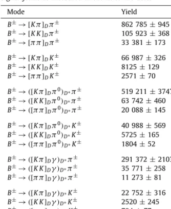
D(∗)_K− _{cross-feed into}

[image:7.612.75.242.89.293.2]

Table 2

Signalyieldsasmeasuredinthefittothedata.

Mode Yield

B±→ [Kπ]Dπ± 862 785±945 B±→ [K K]Dπ± 105 923±368 B±→ [π π]Dπ± 33 381±173

B±→ [Kπ]DK± 66 987±326 B±→ [K K]DK± 8125±129 B±→ [π π]DK± 2571±70

B±→([Kπ]Dπ0)D∗π± 519 211±3747 B±→([K K]Dπ0)D∗π± 63 742±460 B±→([π π]Dπ0)D∗π± 20 088±145 B±→([Kπ]Dπ0)D∗K± 40 988±569 B±→([K K]Dπ0)D∗K± 5725±165

B±→([π π]Dπ0)D∗K± 1804±52

B±→([Kπ]Dγ)D∗π± 291 372±2103

B±→([K K]Dγ)D∗π± 35 771±258 B±→([π π]Dγ)D∗π± 11 273±81

B±→([Kπ]Dγ)D∗K± 22 752±316 B±→([K K]Dγ)D∗K± 2520±245

B±→([π π]Dγ)D∗K± 794±77

calibration sample such that the distributions of these variables match those of selected B−

→

D0

_π

− _{signal decays. It is found} that 71.2% of B−

→

D K− decays pass the companion kaon PID requirement, with negligible statistical uncertainty due to the size of the calibration sample; the remaining 28.8% cross-feed into the B−

→

D(∗)

_π

− _{sample. With the same PID requirement,} approx-imately 99.5% of the B−

→

D

π

− decays are correctly identified. These efficiencies are also taken to represent B−

→

(

D

π

0

_)D

_∗h−

and B−

→

(

D

γ

)D

∗h−signal decays in the fit, since the companion kinematics are similar across all decay modes considered. The re-lated systematic uncertainty is determined by the size of the signal samples used, and thus increases for the lower yield modes. The systematic uncertainty ranges from 0.1% in B−

→ [

K−

π

+

]

DK−to 0.4% in B−

→ [

π

+

π

−

]

DK−.

4.11. Productionanddetectionasymmetries

In order to measure CP asymmetries, the detection asymme-tries for K± and

π

± mesons must be taken into account. A de-tection asymmetry of

(

−

0

.

87

±

0

.

17

)

% is assigned for each kaon in the final state, primarily due to the fact that the nuclear interaction length of K−mesons is shorter than that of K+mesons. It is com-puted by comparing the charge asymmetries in D−

→

K+

π

−

π

− and D−

→

K0

S

π

−calibration samples, weighted to match the kine-matics of the signal kaons. The equivalent asymmetry for pions is smaller

(

−

0

.

17

±

0

.

10

)

%[16]. The CP asymmetry in the favoured B−

→ [

K−

π

+

]

D

π

− decay is fixed to

(

+

0

.

09

±

0

.

05

)

%, calculated from current knowledge of

γ

and rB in this decay [2], with no assumption made about the strong phase,

δ

D_Bπ. This enables the effective production asymmetry, Aeff_B±, to be measured and

simul-Table 4

SystematicuncertaintiesfortheCP observablesmeasuredinafullyreconstructed manner,quotedasapercentageofthestatisticaluncertaintyontheobservable.The

SimuncertaintyonRKKπ/π isduetothelimitedsizeofthesimulatedsamplesused

todeterminetherelativeefficiencyforreconstructingandselectingB−→Dπ−and

B−→D K−decays.

[%] AKπ

K AπK K AK KK Aπ ππ Aπ πK RK K Rπ π RKKπ/π

PID 6.0 4.3 2.0 2.7 10.3 13.8 18.8 0.0

Bkg rate 7.5 1.8 10.2 4.1 18.9 68.7 46.0 0.0

Bkg func 7.6 0.4 4.2 0.4 7.2 9.5 16.7 0.0

Sig func 11.1 0.9 0.8 0.9 14.3 7.9 20.9 0.0

Sim 7.1 0.5 0.2 0.4 5.6 3.5 7.6 174.2

Asym 37.4 52.7 3.7 31.2 2.3 0.1 0.1 0.0

Total 41.5 52.9 11.9 31.6 27.5 71.2 56.9 174.2

taneously subtracted from the charge asymmetry measurements in other modes.

4.12. Yieldsandselectionefficiencies

The total yield for each mode is a sum of the number of cor-rectly identified and cross-feed candidates; their values are given in Table 2. The corresponding invariant mass spectra, separated by charge, are shown in Figs. 1–3.

To obtain the observable RK_Kπ_/π (R_KK_/π_π,π0/γ), which is defined in

Table 1, the ratio of yields must be corrected by the relative effi-ciency with which B−

→

D K−and B−

→

D

π

−(B−

→

D∗K−and B−

→

D∗

π

−) decays are reconstructed and selected. Both ratios are found to be consistent with unity within their assigned uncer-tainties, which take into account the size of the simulated samples and the imperfect modelling of the relative pion and kaon absorp-tion in the detector material.

To determine the branching fraction B

(

D∗0

_→

_D0

_π

0

₎

_{, the yields} of the B−

→

(

D

π

0

_)D

_∗

_π

− _{and B}−

_→

₍

_D

_γ

_)D

_∗

_π

− _{modes are}

cor-rected for the relative efficiencies of the neutral pion and photon modes as determined from simulation. As both of these modes are partially reconstructed with identical selection requirements, the relative efficiency is found to be unity within its assigned tainty, and is varied to determine the associated systematic uncer-tainty. In the measurement of

B

(

D∗

→

D

π

0

₎

_{, the assumption is} made that B

(

D∗

→

D

π

0

₎

₊

_B

₍

_D∗

_→

_D

_γ

₎

₌

_1[29].

The branching fraction

B

(

B−

→

D∗0

π

−

)

is determined from the total B−

→

D∗

π

− yield, the total B−

→

D

π

− yield, the rel-ative efficiencies determined from simulation, and the B−

→

D

π

− branching fraction[29,34]. Both the efficiencies and external input branching fraction are varied to determine the associated system-atic uncertainty.

5. Systematic uncertainties

The 21 observables of interest are free parameters of the fit, and each of them is subject to a set of systematic uncertainties that result from the use of fixed terms in the fit. The systematic

uncer-Table 3

SystematicuncertaintiesfortheCPobservablesmeasuredinapartiallyreconstructedmanner,quotedasapercentageofthestatisticaluncertaintyontheobservable.

[%] AKKπ ,γ A

Kπ ,γ

π AKπ ,π 0

K A

Kπ ,π0

π A

C P,γ

K A

C P,γ

π AC P,π 0

K A

C P,π0

π RC P,γ RC P,π 0

RKKπ ,π/π 0/γ

PID 4.0 11.4 4.4 3.8 9.1 5.0 4.7 4.4 22.0 16.9 74.8

Bkg rate 3.5 1.6 3.2 3.6 40.8 3.5 16.5 5.7 114.0 41.9 180.3

Bkg func 8.9 1.0 3.7 0.7 24.4 1.6 27.1 1.3 42.6 25.0 417.3

Sig func 4.8 3.9 2.9 3.9 10.9 3.6 3.7 4.3 24.6 13.8 148.4

Sim 3.1 1.1 2.1 1.9 6.5 0.9 4.3 2.9 23.5 15.3 153.8

Asym 29.9 6.8 34.1 19.4 1.0 9.4 2.2 26.1 1.4 0.6 1.9

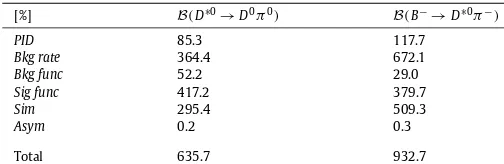
[image:7.612.302.554.127.210.2] [image:7.612.31.554.659.746.2]

[image:8.612.42.294.100.182.2]

Table 5

Systematicuncertaintiesforthebranchingfractionmeasurements,quotedasa per-centageofthestatisticaluncertaintyontheobservable.

[%] B(D∗0_→D0_π0_{) B(B}−_→D∗0_π−₎

PID 85.3 117.7

Bkg rate 364.4 672.1

Bkg func 52.2 29.0

Sig func 417.2 379.7

Sim 295.4 509.3

Asym 0.2 0.3

Total 635.7 932.7

tainties associated with using these fixed parameters are assessed by repeating the fit many times, varying the value of each external parameter within its uncertainty according to a Gaussian distribu-tion. The resulting spread (RMS) in the value of each observable is taken as the systematic uncertainty on that observable due to the external source. The systematic uncertainties, grouped into six categories, are listed in Tables 3 and 4 for the CP observables measured in a partially reconstructed and fully reconstructed man-ner, respectively. The systematic uncertainties for the branching fraction measurements are listed in Table 5. Correlations between the categories are negligible, but correlations within categories are accounted for. The total systematic uncertainties are summed in quadrature.

The first systematic category, referred to as PID in Tables 3

−

5, accounts for the uncertainty due to the use of fixed PID efficiency values in the fit. The second category Bkgratecorresponds to the use of fixed background yields in the fit. For example, the rate of B0

_→

_D∗−

_π

+ _{decays is fixed in the fit using known branching}

fractions as external inputs. This category also accounts for charm-less background contributions, each of which have fixed rates in the fit. The Bkgfuncand Sigfunccategories refer to the use of fixed shape parameters in background and signal functions, respectively; each of these parameters is determined using simulated samples. The category Simaccounts for the use of fixed selection efficien-cies derived from simulation, for instance the relative efficiency of selecting B−

→

(

D

π

0

_)D

_∗

_π

−_{and B}−

_→

_D

_π

−_{decays. The final}

cat-egory, Asym, refers to the use of fixed asymmetries in the fit. This category accounts for the use of fixed CP asymmetries and detec-tion asymmetries in the fit, as described earlier.

6. Results

The results are

AK_Kπ,γ

= +

0

.

001

±

0

.

021 (stat)

±

0

.

007 (syst)

AπKπ,γ

= +

0

.

000

±

0

.

006 (stat)

±

0

.

001 (syst)

AK_Kπ,π0

= +

0

.

006

±

0

.

012 (stat)

±

0

.

004 (syst)

A_πKπ,π0

= +

0

.

002

±

0

.

003 (stat)

±

0

.

001 (syst)

ACP_K,γ

= +

0

.

276

±

0

.

094 (stat)

±

0

.

047 (syst)

ACP_π,γ

= −

0

.

003

±

0

.

017 (stat)

±

0

.

002 (syst)

ACP_K,π0

= −

0

.

151

±

0

.

033 (stat)

±

0

.

011 (syst)

ACP_π,π0

= +

0

.

025

±

0

.

010 (stat)

±

0

.

003 (syst)

RCP,γ

=

0

.

902

±

0

.

087 (stat)

±

0

.

112 (syst)

RCP,π0

=

1

.

138

±

0

.

029 (stat)

±

0

.

016 (syst)

RK_Kπ_/π,π0/γ

=

(

7

.

930

±

0

.

110 (stat)

±

0

.

560 (syst)

)

×

10−2

B

(

D∗0

→

D0

π

0

)

=

0

.

636

±

0

.

002 (stat)

±

0

.

015 (syst)

B

(

B−

→

D∗0

π

−

)

=

(

4

.

664

±

0

.

029 (stat)

±

0

.

268 (syst)

)

×

10−3 AK_Kπ

= −

0

.

019

±

0

.

005 (stat)

±

0

.

002 (syst)

AK K_π

= −

0

.

008

±

0

.

003 (stat)

±

0

.

002 (syst)

AK K_K

= +

0

.

126

±

0

.

014 (stat)

±

0

.

002 (syst)

Aπ π_π

= −

0

.

008

±

0

.

006 (stat)

±

0

.

002 (syst)

Aπ π_K

= +

0

.

115

±

0

.

025 (stat)

±

0

.

007 (syst)

RK K

=

0

.

988

±

0

.

015 (stat)

±

0

.

011 (syst)

Rπ π

=

0

.

992

±

0

.

027 (stat)

±

0

.

015 (syst)

RK_Kπ_/π

=

(

7

.

768

±

0

.

038 (stat)

±

0

.

066 (syst)

)

×

10−2

.

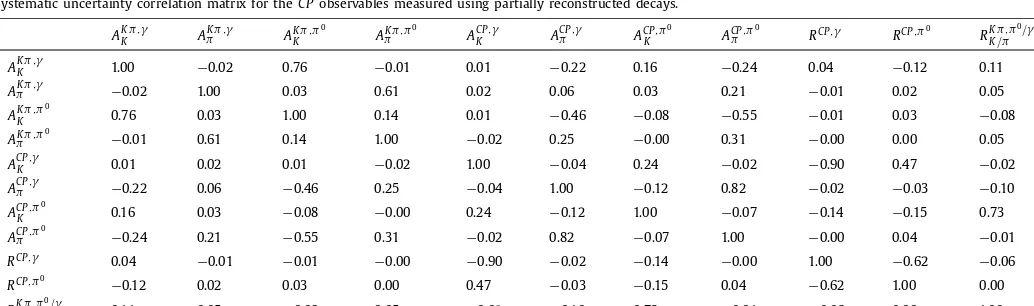
The results obtained using fully reconstructed B−

→

Dh− decays supersede those in Ref. [12], while the B−

→

D∗h− results are reported for the first time. The statistical and systematic corre-lation matrices are given in the appendix. There is a high de-gree of anticorrelation between partially reconstructed signal and background components in the fit, which all compete for yield in the same invariant mass region. The anticorrelation between the B−

→

(

D

π

0

_)D

_∗h− _{and B}−

_→

₍

_D

_γ

_)D

_∗h−_{CP observables is visible} in Table 6of the appendix. The presence of such anticorrelations is a natural consequence of the method of partial reconstruction, and limits the precision with which the CP observables can be mea-sured using this approach.

The value of AK K_K has increased with respect to the previous re-sult[12], due to a larger value being measured in the

√

s

=

13 TeV data. The values measured in the independent

√

s

=

7, 8 and 13 TeV data sets are consistent within 2.6 standard deviations. All other updated measurements are consistent within one standard deviation with those in Ref.[12].

Observables involving D

→

K+K−and D

→

π

+

π

− decays can differ due to CP violation in the D decays or acceptance effects. The latest LHCb results [45] show that charm CP-violation ef-fects are negligible for the determination of

γ

, and that there is also no significant difference in the acceptance for the two modes. Therefore, while separate results are presented for the B−

→

Dh− modes to allow comparison with previous measurements, the com-bined result is most relevant for the determination of

γ

. The RK K and Rπ π observables have statistical and systematic correlations of

+

0.07 and

+

0.18, respectively. Taking these correlations into ac-count, a combined weighted average RCP _{is obtained}

RCP

=

0

.

989

±

0

.

013

(

stat

)

±

0

.

010

(

syst

) .

The same procedure is carried out for the AK K

K and Aπ πK observ-ables, which have statistical and systematic correlations of

+

0.01 and

+

0.05, respectively. The combined average is

ACP_K

= +

0

.

124

±

0

.

012

(

stat

)

±

0

.

002

(

syst

) .

The observables RCP,π0

and ACP,π0

(RCP,γ _{and A}CP,γ_),

mea-sured using partially reconstructed B−

→

D∗h−decays, can be di-rectly compared with the world average values for RCP+

≡

RCP,π0

and ACP+

≡

ACP,π0

(RCP−

≡

RCP,γ _{and A}

CP−

≡

ACP,γ_{) reported}

by the Heavy Flavor Averaging Group [3]; agreement is found at the level of 1.5 and 0.4 (1.1 and 1.4) standard deviations, respec-tively. The values of RCP,π0

and ACP,π0

considerably improve upon the world average precision of RCP+ and ACP+, while the mea-surements of RCP,γ _{and A}CP,γ _{have a precision comparable to the}

previous world average.