Adaptive Estimation Techniques for Hidden Markov Models

Adaptive Estimation Techniques

for

Hidden Markov Models

Vikram Krishnamurthy

September 1991

A thesis submitted for the degree of Doctor of Philosophy of the Australian National University

Department of Systems Engineering

Research School of Physical Sciences

and

Engineering

Chapter

5

Signal Processing of Semi-Markov

Models with Decaying States

5.1

Introduction

Hidden Markov models with discrete states have been widely used to model noisy physical systems in communication systems, speech and sonar processing and more recently in biological signal processing of ion channel currents in cell membranes. In these models, the transition probabilities and symbol probabilities are assumed to be independent of the time. Thus the time the homogeneous Markov chain spends in a state is statistically determined by the geometric probability mass distribution [7]. In certain physical systems, however, the transition and/or symbol probabilities are a function of the time to the last transition. Such processes are called semi-Markov processes [8].

One example of a semi-1brkov process, are certain biological fractal signals from ionic channel current measurements, as has been studied in an earlier paper [56]. Here the signal behaviour when appropriately time scaled is independent of the bandwidth of the aliasing filter and sampling rate. Its 'ruggedness' is characterized by its fractal dimension. In such a case, fractal models [56], [9], [10), with their time-varying transition probabilities dependent on the time to the last transition become more appropriate than scalar Markov models that are homogeneous, i.e., with time-invariant transition probabilities. Another example is the discrete-semi Markov chain with Poisson-distributed transition times. Such models are widely used in the modelling of seismic signals and images [67), [58).

97 More sophisticated hidden discrete semi-Markov stochastic processes encountered in some physical systems are such that subsequent to a step transition governed by transition probabilities dependent on the time to the last such step transition, there is exponential (or other) decay until the next step transition. That is, there is memory in the signal model which can be reasonably modelled by some dynamical filter, possibly nonlinear. Signal processing for hidden semi-Markov processes with memory have not been well developed or studied.

The initial motivation for our work has been the need to study certain cell mem-brane currents which exhibit obvious exponential decay behaviour between step transi-tions. These are similar to piecewise constant signals passed through a dynamic channel as studied in telecommunication literature [59), save that here the residual memory prior to the next transition appears negligible, or equivalently there is negligible intersymbol interference. In the telecommunication channel situation, the effective number of discrete states and processing effort grows exponentially with the memory length, whereas with our channels since the memory of a past step transition is taken to be negligibly small compared to a new step transition, we show that the channel memory does not affect the computational effort. The schemes we propose seek to estimate the decay rates between step transitions, the time varying transition probabilities of the imbedded stochastic pro-cess, and the noise statistics if unknown. This work is preliminary to current investigations where less apparent, more complex resonant dynamics are conjectured.

This work also has been in part motivated by our curiosity to see if HMM signal processing techniques naturally generalize to semi-Markov models and if so, whether there is any incentive for working with such generalized techniques instead of standard HMM techniques as currently used in many areas of signal processing. Our previous work has been with first and higher order HMM and Hidden Fractal Model representations of ion channels in cell membranes [56), [5) and forms the basis of this work.

98 In this chapter, we first recall from

[.56]

reformulations of the scalar time-varying HMM as a 2-vector first order homogeneous HMM. The reformulation is carried out by augment-ing the underlyaugment-ing scalar stochastic process with the time spent to the last transition. However unlike [56], due to the presence of the channel memory until the next transition, the symbol probabilities are also a function of the time to the last transition. This allows us to cope with memory in the case when the residual memory (memory effects at a new transition) are negligible. This is indeed the case in many biological applications [11], [12), [13) where the decay time constants are much smaller than the average duration time in a state. Our main task then is to generalize the techniques in (56] to cope with symbol probabilities which are a function of the time to the last transition. In the most general formulation, we allow for different memory characteristics for different states of the semi-Markov chain. It is theoretically possible in some time-varying models that the number of possible discrete-states for the time to the last transition is the number of observations in the data set. However, it turns out that in many models with practical significance (e.g. fractal models) the number quantization levels for this time variable can be significantly reduced via aggregation.

Once the hidden semi-Markov model has been formulated as an augmented homoge-neous HMM, known HMM techniques such as the vector versions of the forward-backward algorithm along with the Baum-Welch [17] [18], [19] re-estimation formulae are applied to achieve improved estimates of both the signals and the signal model parameters, in-cluding signal levels, transition probabilities and noise statistics. Repeated application of the forward-backward algorithm and the re-estimation formulae achieves maximum a posteriori probability (MAP) or conditional mean ( CM) signal estimates (5], (52], [21). To "learn" the signal model parameters with any degree of certainty, there must be sufficient "excitation" of all the possible transitions between the various states. Once the augmented HMM is estimated, it is a straightforward procedure to compute the signal channel mem-ory characteristics in terms of the filter used to model the memmem-ory, and the parameters of the time-varying functions that govern the transition probabilities.

99

faster convergence and improved state estimates. We also deal with the special case when the dynamical filters are identical for the various states of the semi-Markov process and the states are equally spaced. In such a case it is possible to further reduce the number of estimated parameters. The resulting EM formulation leads to improved signal estimates.

The chapter is organized as follows: In Section 5.2 we formulate the Hidden semi-Markov problem as a 2-vector homogeneous HMM problem and review learning and esti-mation objectives of HMM schemes. In Section 5.3, estiesti-mation and re-estiesti-mation schemes are presented for vector HMMs. In Section 5.4, we present simulation studies. Finally, some conclusions are presented in Section 5.5.

5.2

Problem Formulation

In this section first the signal model is described. Next we characterize noisy channels with memory for the scalar semi-"Markov process and reformulate the scalar semi-Markov Hidden Markov models as augmented 2-vector Hidden Markov Models. Finally we recall Hidden Markov Model learning and estimation objectives and describe processing schemes for our signal models.

5.2.1

Signal Model

Here scalar finite-state semi-Markov models are described, with an illu~tration of the fractal model. Then the noisy channel is formulated as a dynamical, possibly nonlinear, filter.

Multi-state semi-Markov model:

Consider a discrete-time, finite-state stochastic process sk, k ~ 0, where for each k, Sk is a random variable taking on a finite number N8 of possible states qt. ••• ,qN,· Assume that the transition probabilities aij(k) at time k defined as a;j(k)

~

P(sk+l

=

qilsk

=

q;) being functions of the time to the last transition at time k, denoted tk, are functions of the form:

aij(tk): tk ~---+ [0, 1] for i,j E [1,N8 ] (5.1)

100 such as Ti

=

i or Ti

=

2i. ·without any computational effort and memory constraints, it

would be reasonable to take Ti as the integer i, for i = 1, ... , Nt. An upper bound on

Nt is the total number of observations in the data set. However, as described later, state aggregation allows Nt to be bounded by more realistic values. Notice that when aij(tk) is independent of tk. the transition probabilities are independent of time, and sk reduces to

a homogeneous first order Markov process.

Fractal model example: Fractal stochastic processes [56], [9], [10] are used to model the opening and closing of channel gates in cell membranes. For a continuous-time fractal stochastic process, the rate of transition from one state to another is a function of the time scale in which it is observed. The transition rate matrix of a two state fractal process is of the form

(5.2)

where t is the time to the last transition. D1. D2 are termed the fractal dimensions and k1. k2 are the initial setpoints. For a physically and mathematically plausible density function, 1 ~ Di

<

2 in (.5.2). The corresponding transition probabilities are the solutions of the matrix differential equation

A(t)

=

H(t) A(t), A(O) =I

where A(t)

=

(aij(t), aij(t)

=

P(st

=

qiJs0

=

qi)). In general it is not possible to obtain the transition probabilities in a closed form. However when Dt

=

D2, then A(t)

=

exp(f~H(u)du) and the transition probabilites can be obtained in a closed form.

The discrete-time version of the continuous-time fractal model is obtained by ap-propriate lowpass (anti-aliasing) filtering and sampling at greater than or equal to the Nyquist sampling rate. The filter bandwidth then determines the temporal resolution. Let Is

=

1/Ts be the sampling frequency. The discrete transition probabilities of the sampled fractal process cannot be obtained in a closed form in general. However, it is easily shown that,

101

a22(tk) increase and asymptotically approach 1; a12(tk), a21(tk) asymptotically approach 0. We shall also use (5.3) subsequently when dealing with state aggregation.

Notice that when Di

=

1, the transition probabilities are independent of time and Sk

reduces to a homogeneous first order Markov process.

Noisy measurement process with truncated memory:

Consider the case where the semi- Markov process Sk is filtered yielding rk and is imbedded in noise, that is, indirectly observed by measurements Yk· Denote the sequence

Yl!Y2,···,Yk byYk.

Recall that Sk is a semi-Markov process with states qi, i = 1, ... , N6 • The filtered process Tk is dependent on the current state value of Sk, denoted qi, and the time to the

last transition of sk denoted tk. We denote this dependence as

(5.4)

Here f(.) is constrained to any smooth function with the following requirements:

(i) Negligible residual memory: if tk = 1 then the value of rk is independent of the value of rk_ 1.

(ii) Identifiability: for some tk and i -::j; j, f(qi,tk) -::j; f(qj,tk)·

A special case of interest is when the measurements Yk consist of rk corrupted by zero mean, normally distributed white noise as follows:

(5.5)

Exponentially decaying states example [11], [13]: Consider the case when the channel is modelled as a bank of IIR filters Ci( q-1 ) depending on the state qi of the semi-Markov process. Then rk is of the form

(5.6)

102

exponential decay between step transitions. Here q1 is termed the ground state and does not decay exponentially. For tk

=

1, rk is usually considered as qi since the rise time from the ground state to the state level qi is much smaller compared to the decay time. Also typically the decay time in a state is much shorter than the duration time in a state so that the residual memory just prior to a transition is negligible.

5.2.2 Reformulation as Hidden Markov Model

First the semi-Markov process is reformulated as a vector homogeneous Markov process. Then we deal with the observations of this imbedded Markov process obtained through the noisy channel with memory ( 5.4) as a Hidden Markov process.

Formula ton of semi-Markov process as vector homogeneous Markov process The class of scalar semi-Markov models in (5.1) can be modelled as a homogeneous first order 2-vector Markov process as follows: Define the 2-vector process Sk as Sk

=

(tk,sk)

for each k

:?:

0. Clearly Sk is a finite-state process with N = N8 Nt states. Here Nt is taken as the ma.ximum duration time in any state considering the observation sequence of length T.

It is easily shown that the 2-vector stochastic process Sk, as defined above with Ti

=

i

for i

=

1, ... , Nt is a homogeneous, first order Markov process (see [56]). Notice that

{ tk

+

1 if sk+l

=

Sk and tk

<

Nt

tk+l

=

1 otherwise

(5.7)

So tk+I depends only on tk, sk and Sk+I· Also from (5.7) the transition probabilities for the homogeneous vector process sk are

which are independent of k.

if sk

=

(rh,qi) and sk+l

=

(rh

+

1,qi)i 1::::; Th

<

Nt

if sk

=

(rh,qi) and sk+l

=

(1,qj), i

=f.

j, 1::::; Th::::; Nt

otherwise

(5.8)

103 states in the saturation region is possible as discussed below. 0

Notation: Denote the set of N = N8 Nt states {(rl,qi), ... ,(rNt,qN.)} as

{Qt, Q2, ... , QN }, although, not necessarily in the same order. We will denote elements of this set by integer subscripts, usually morn. Also for Qm

=

(rh,qi) and Qn

=

(rz,qi) where m, n E [1, N], rh, TJ E [1, Nt], qi, qj E [1, Ns], denote the transition probabilities of the homogeneous S k process by

(5.9)

Hidden semi-Markov Models with truncated channel memory

Consider a semi-Markov processes observed through the noisy channel with memory defined by (5.4). Assume that the semi-Markov process Sk and hence the associated vector Markov process Sk = (tk, sk) are hidden, that is indirectly observed by measurements Yk· The vector of probability functions b(.) = (bm(.)) = P(YkiSk = Qm) where Qm = (rh,qi) is a function of the time to the last transition rh. So

(5.10)

Also assume the independence property

(5.11)

Further, assume that the initial state probability vector 1!:. =

(7rm)

is defined from

(5.12)

The transition probabilities A are defined as in (5.9). The vector HMM for the Sk process is denoted>.= (A, b(.),l!:.). Of course>. also denotes the Hidden semi-Markov model for the

sk

process.

104 Notice that the independence assumption on the model reflects itself here as an indepen-dence 'whiteness' assumption on wk. The theory developed in Section 5.3.3 and simula-tions presented subsequently deal with this special case. The theory and algorithms in the rest of this chapter, however, do not rely on this additive normally distributed noise assumption.

5.2.3 Aggregation

In proving that skis a homogeneous Markov process above, it is assumed that Ti = i and

Nt is the maximum duration time in any state. Since we may not know this value we

can set Nt = T, the length of the entire observation sequence, but then the number of states N = Nt Ns will be excessive for computational purposes. Is it possible to quantize the time to the last transition to Nf states, where Nf

< <

T with negligible error? We propose to do so by "aggregating" [54] the states (TN', qi), ( TN'+l, qi), ... , ( TNo qi) into a

t t

aggregated state

(5.13)

Aggregation Property: We have proved in [56] that the above aggregation leads to negligibly small errors for a certain class of functions aij( tk) defined in ( 5.1) satisfying for arbitrary small E

>

0

(5.14)

More specifically, the fractal model with transition probabilities that exponentially converge, see 5.3, and the discrete semi-Markov process with Poisson distributed transition times satisfy (5.14) and so can be aggregated. Simulations show that in most cases for such processes, choosing Nt so that E

<

0.05 is adequate. For the rest of this chapter we set Nt

=

N;

<:

<

T where N; is suitably large (usually less than 50) to result in negligible error. Of course, now (5.7) is modified as

if sk+l = sk and tk

<

Nt if .sk+l = Sk and tk = Nt

otherwise

105

Transition probability matrix sparseness: Notice that with Th

=

h for h

<

Nt

=

Nf,

the relationship between (5.1) and (5.9) is

(5.16)

Clearly A has (Ns Nt)2 _{= N}2 _{elements. However, since tk+l is restricted as in (5.15) to}

only three possible values, simple calculations show that (N2 - N; Nt) elements of A are zero. For i,j E [1, ... N8 ], only the following elements of A are not necessarily zero:

(5.17)

Consequently, in any scheme to estimate A, only the N; Nt elements of A in (5.17) need be estimated.

5.2.4 Learning and Estimation Objectives

Given the semi-Markov signal model reformulated as a homogeneous Markov model as described above, and given observations Yl, y2, .•. , Yk denoted Y k, there are three inter-related HMM problems which can be solved [52], [21] and interpreted to yield results for the underlying semi-Markov process.

1. Evaluate the likelihood of a given model Ai generating the given sequence of data, denoted P(Y k

I

Ai). This allows com pari son of a set of models { Ai} to select the most likely, given the observations.

2. Estimate signal statistics such as a posteriori probabilities for an assumed model

A

and data sequence. For a fixed interval T, estimate

(5.18)

From 'i'kjT(m), state sequence estimates conditioned on A, denoted {Sk!A}, such as maxi-mum a posteriori (MAP) can be generated as

srrAP

=

Qn where n

=

arg max 'i'kiT(m)

1$m$N

Of course if Qn = ( Th, qj) then .s~IAP = qj in (5.19).

106 Also in the special case when the noise is Gaussian, estimate its mean and variance: For the state Qm = ( Th, qi), the estimated mean

Tim

is obtained as (see [18])

(5.20)

and the estimated variance is calculated as

(5.21)

3. Processing of the observations based on a model assumption .X, and adjustment (re-estimation) of the model parameters (functions) (A, b(.),lL), such that the likelihood of the updated model X= (A, b(.),:ZL) given the observation sequence, P(YTIX)

>

P(YTI.X), and repeating until convergence. The objective is to achieve the most likely model _xML

amongst the set A= (A, b(.),lL), given the observations.

5.3

Estimation and Re-estimation

We now proceed to solve Problems 1 to 3 above for the hidden semi-Markov model refor-mulated as a HMM. The formulae of this section turn out to be identical to more familiar ones for scalar HMMs, as in

[5],

but with scalars sk replaced by 2-vectors Sk and the states %qi replaced by Qm,Qn which can be associated with the pair of scalar states (rh,qi)

and

(Tz,qj)·

5.3.1

Forward-backward Procedure

Consider an observation sequence Y T of length T and assumed signal generating model .X.

Forward and backward vector variables are defined as probabilities conditioned on the model .X, form= 1, 2, ... , N as follows:

flk

=

(ak(m));

~

=

(f3k(m));

,6.

ak(m)

=

P(Yk,Sk

=

Qmi.X)

,6.

-f3k(m)

=

P(Yk!Sk

=

Qm,.X)

where Y k denotes the future sequence Yk+l, Yk+2• ... , YT·

Recursive formulae for f!k and

f!.k

are readily calculated [56], [5], [21] as

ak(n)

=

(~

1

ak-l(m)amn) bn(Yk),

a1(n)

=

7rnbn(Yt)

N

Pk(m)

=I:

amnbn(Yk+l)t'k+l(n), t'T(m)

=

1

n=l

107

(5.23)

where Qn

= (

Th, qj) for any 1

:S

Th

<

Nt. Updating f!k and~ requires the order of N2 M multiplications and additions at each time instant k because only N2 _{M components of A} are not necessarily zero, see (5.17).

The optimal a posteriori probabilities associated with Problem 2 are given from [5], [21]

ak(m)f3k(m)

!k=(!k(m)); /k(m)= N , m=1,2, ... ,N.

- Lm=l ak(m),f3k(m)

(5.24)

Then using (5.19) we obtain MAP fixed-interval smoothed estimates. The likelihood function, which is the end result of the Problem 1, is calculated as

N

LT

~

P(YTj,\) =

I:

aT(m).

(5.25)

m=l

5.3.2

Baum-Welch Re-estimation Formulae

Define the joint conditional probability

(5.26)

Re-estimation of A, 1L are given from

(5.27)

In updating the vector of probability functions b(.), it is reasonable to do this at a finite number of points v1 , v2 , ••• , VM in the range of the signals Yk· Quantizing Yk to these levels, gives a quantized signal Yh and allows re-estimation of bm(vj) as

(5.28)

108 It is proved in [52] that with the re-estimation formulae (5.27), (5.28), the model

X= (A, b(.),lE) is more likely than .X, given the observations, in that P(YTIX) ~ P(YTI.X).

Remark: The Baum-Welch algorithm belongs to a class of numerical algorithms called Expectation Maximization (EM) algorithms [20], [15]. In Section 5.3.3, we shall consider other more suitable EM algorithms in the presence of Gaussian noise. 0

Determining transition probability parameters and filter coefficients: Here we describe how the parameters that govern the time-varying transition proba-bilities and the filter coefficients are obtained from the Baum-Welch estimates.

Transition Probability parameters: Note that from the Baum-Welsh estimate A of A, the parameters of the function a;j (see (5.1)) are obtained by fitting functions of

the form aij to a(h,i),(h+l.j)• 1 ::; rh

<

Nt (see (5.16)) in a least squares sense. However,

because of the finite length of the observation sequence, for large values of rh it is often the

case that there are not sufficient such transitions to get a reliable estimate of a(h,i),((.),j)· Also, we ignore a(l,i),((o),j) since it includes all events that happen faster than our time

scale of interest, this time scale being determined by the bandwidth of the lowpass filter used. Thus typically for a few thousand observations, it makes sense to use a(h,i),(h+IJ)

only for 2 ::; rh ::; 5 (say) in the least squares fit.

Filter coefficients: If the functional form of the dynamical filter is known then the actual parameters can easily be obtained by least squares fitting. For example if the channel is modelled by IIR filters (see ( 5.6), then the coefficients of the IIR filters Ci( q-1 ) are calculated from the estimates of b(.) as follows: Let b'h,i

=

maxi bh,i( Vj)

. Also define the vectors b£ = [bR(i)+2,i, ... , b}lt,i] and the vector of filter coefficients c(

i)

=

[co( i), ... , cR(ij(i)jT.

Then estimates of the filter coefficients are obtained by solving for c(i) from

b'!' - B _{t -} c(i)

in a least squares sense where

b'R(i)+l,i b'R(i),i bl* 0

••

B= b'R(i)+2.i b'R(i)+l,i

b2* 0

••

(5.29)

b~, 2 °

109

5.3.3 Fast converging Re-estimation Algorithm for Gaussian Noise

In this subsection we present efficient methods of re-estimating bm (. ). When these schemes are used in conjunction with the Baum- Welch equations for re-estimating the transition probabilities, convergence rates are significantly improved.

Efficient re-estimation in Gaussian noise (Scheme 1): When the Markov process is imbedded in Gaussian noise, then the EM algorithm can be used to directly re-estimate the mean llm and variance 0"~ instead of re-estimating theM parameters bm( Vj),j = 1, ... ,M

for each m. Once llm and 0"~ have been calculated using (5.20) and (5.21), the Gaussian density bm(.) can be updated as

where

Qm

= ( Th, qi).

Fast converging algorithm (Scheme 2): We now present a modification of the above EM algorithm for even faster convergence.

It is proved in [23] that if the observations were obtained by adding white Gaussian noise to an imbedded independent process (rather than a markov process) then the con-vergence rates of the resulting EM re-estimation equations for the mean and variance can be improved as follows:

Define the reestimated mean and variance obtained from the standard EM re-estimation formulae after the pth pass as '!j;(P) where '!j;(P) = (7Im, 0"~). Then the standard EM

re-estimation formulae can be written as

where G represents the EM re-estimation (see [15], pp 85-88). Let

"'ii}P)

be the re-estimated model obtained after the pth pass of the fast converging EM algorithm. Then the estimates from the p

+

1 pass of the fast converging EM algorithm are

esti-110 mates are chosen close enough to 'lj;, local convergence occurs for 0 ~ 'T]

<

2. Asymptotical optimal rates of convergence occur for some 'T]* with 1

<

'T]*

<

2. Typically, if the compo-nent densities are well separated, 1]"' is near 1 and convergence is fast, otherwise 'T]* is 2

and convergence is slow.

We conjecture that these results generalize to the case where the imbedded process is a Markov processes as follows: Let

1iJ

be the re-estimated mean and variance after the pth pass. Then

(5.30) Here '!jJ(P+l) = (i1m,O'~) is calculated from (5.20) and (5.21) and 0

<

'T]

<

2. Computer

simulations show the that the rates of con vergence are indeed increased when using the above modified algorithm with 1

<

17

<

2. Also if the convergence is fast for the standard case, choosing 'T] close to 2 does not significantly slow convergence. However, most often

the initial model and hence the initial mean and variance estimates are chosen arbitrarily and may be quite different from the most likely values. In such cases choosing 'T] close to

2 significantly improves convergence rates. So we recommend in general that 'T] be chosen

close to 2.

Exponentially Decaying States: When it is known that the Markov states de-cay exponentially as in (.5.6) then the EM algorithm can be used to directly obtain the exponential decay constants c;( i), i = 1, ... N8 •

E step: This involves computing Q(>., 'X) which is the expectation of the log of the likelihood function of the fully categorized data (see [20], [15] for details). Here

N N T-l N

Q(>.,'X)=

L L

L(dm,n)loglimn+ L1't(n)log""'n+Q2 (5.31)

m=l n=l k=l n=l

where

(5.32)

Because we apriori assume that the states decay exponentially according to (5.6), it follows thatj1hi =

.

(ct(i))h-tj71i, h

=

l, ... ,Nt, i

=

1, ... ,Ns. So Q2 can be rewritten as

'

111

M step: This involves finding

X

to maximize Q( A,

'X).

Maximizing the first two terms on the right hand side of ( 5.31) yields the standard Baum-Welch equations for re-estimating ii'mn and 1Fm. Now consider maximizing the third term in (5.31) namely

'h

which is expressed as (5.33). Solving for 8Q2/ o]11,i = 0 yields

(5.34)

Also solving for 8Q2/8c}(i) = 0 yields

N M N M

L L

'Yk(h,i)(h- l)(c1(i))h-2 _{Yk =}

L L

_{'Yk(h,i)(h -1)(CI(i))2 h-3j1(1,i) (5.35)}

k=lh=l k=lh=l

Based on (5.34) and (.5.35), we now propose three methods for re-estimating c1(i) and

j!(l, i). These methods are also used in Chapter 6.

1. Standard EM Re-estimation: To solve for c1 ( i) and j!(l, i), we need to solve (5.34) and (5.35) simultaneously. This can be done for example by substituting (5.34) forj!(l,i) in (5.35). Then the resulting equation can be solved numerically to yield estimates for ct(i) and then j!(l,i) can be obtained from (5.34). The disadvantage of this method is that we need to numerically solve a 3 Nt - 4 order polynomial equation for ci(l).

2. Block Component Re-estimation [67]: Like the standard EM algorithm, this scheme ensures that the likelihood function improves after each pass. Here c1 ( i) and j!(l, i) are updated in alternate passes. So we keep j1(l,i) constant in one pass and update c1

(i)

in

that pass. Then we keep c1 ( i) constant in the next pass and update j1(1, i) and so on. Note

that the transition probabilities are updated every pass since their re-estimation equations are independent of maximizing Q2 •

3. Quasi-EM Re-estimation: This scheme is similar to that proposed in [65) and (66). In re-estimating ct(i) and 7I(l,i), we use (5.34) and (5.35) with ct(i) and J1(l,i) in the right hand sides of the equations replaced by c1 ( i) and J.L(l, i). Simulations show that

this quasi-EM algorithm yields acceptable results. Of course, this algorithm is also much simpler to implement than the standard EM algorithm since (5.34) and (5.35) do not need to be solved simultaneously. So only a 2 Nt - 3 order polynomial equation needs to be solved numerically.

112

c1 ( i) satisfying 0

<

c1 ( i) ~ 1. While we have not been able to prove uniqueness, extensive

simulations seem to confirm that there is a unique c1 ( i) in the range 0

<

Ci'(

i)

~ 1. In any case, if more than one solution does exist, then in theM step we choose that solution which maximizes Q2.

Equally spaced means: In some biological examples [13] it is apriori known that the means f.Lh,i, i = 1 ... , Ns are equally spaced. An example is when the Markov states are equally spaced and the filters are identical. We can exploit the knowledge of the means being equally spaced to speed up convergence and further decrease the number of parameters estimated as follows: Let 6.

~

Qi+l - q;, i = 2, ... , N8 - 1 be the state separation. Since the filters are such that the means are equally spaced, let f.Lh,i+l - f.Lh,i = t:lh, i

=

1, ... , N8 - 1. So we only need estimate 6.h and f.Lh,l for each h, h

=

1, ... , Nt.

It is proved in the appendix that the maximization (M) step of the EM algorithm yields estimates of these as

- L.I=llk(h, 1) Yk h N

llh 1

=

T ,

=

1, · · ·, t

· Lk=l rk(h, 1) (5.36)

(5.37)

Hence by re-estimating i1h,l and 6.h at each pass we can compute

Usually in biological examples the 'baseline' state does not decay, i.e., J.Lh,l = 0, h = 1, ... , Nt. In such cases use (.5.36) to re-estimate i1h, 2• Then compute t:lh from (5.37) with

71h,

2 replacing 7Ih,l·

More generally, if the function g( 6.h, i) defined by

(5.38)

is known, then it is shown similarly to the proof in the appendix that 7Ih,l is obtained from (5.37) and that t:lh is computed by solving

(c) Y'k

a

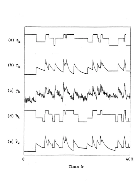
400

Time k

Fig.

5.1

Performance of Scheme 2 on noisy exponentially

decaying Markov signal

[image:19.602.66.515.87.672.2]

114

5.4

Computer Studies

First we illustrate the effectiveness of the algorithms presented in this chapter on com-puter generated data. In particular we compare likelihood functions and signal estimates. Then we present results of the above algorithms on a segment of data obtained from cell membrane currents. See [56] for a brief description of associated implementation aspects including Adaptive scaling.

Remark: When modelling finite segments of data certain transitions may only occur rarely or perhaps not at all. The transition probabilities for these "rare events" cannot be reliably re-estimated using any statistical approach due to the lack of sufficient "exci-tation". Thus in interpreting model estimation results via there-estimation equations on finite data, not too much credence should be given to the estimation of low probability

events. 0

Hidden Fractal Model data: See Chapter 4 for results on the simulation perfor-mance of the algorithms on fractal data.

Hidden Markov model with Decaying states:

Example 1: In this example we illustrate the performance of the proposed re-estimation schemes.

A 10000 point four-state first order Markov chain was generated with transition prob-abilities aii

=

0.97, with the states at 0, 1, 2 and 3. The resulting Markov chain was

exponentially filtered with decay constants [c1 ( 1), c1 (2), c1(3), c1( 4))

=

[1.0 0.98 0.95 0.90) where c1(i) are defined in (5.6). Also c0(i) = 1 in (5.6). Zero mean white Gaussian noise of standard deviation (J'w = 0.5 was added to the exponentially filtered signal.

Fig.5.1 a,b and c show 400 points of the Markov chain Sk, the filtered chain rk, and the observations Yk respectively. After applying Scheme 2 of Section 5.3.3 for 40 passes, the resulting MAP state estimates Sk for the corresponding 400 points is plotted in Fig.5.1d.

170r---~~---~---P---~

No. of errors per 1000

points 130 120

110

100

901 ₂

Baum Welch

.-·-·-·-·-·-·-·-·-·-·-·-·-·-·-·-·-·-·-·-·-·

Scheme 2, £ = 1. 9

- 1 1 __ ,_,_ _______ _

£- . _,

,,

·-·-·-·

No. of passes

8 Scheme 1

9 10

.7000~--~--~~--~---~--~----~--~--~

-6500

'

Log L -6000 \

\

- 5500 '· Scheme 1, Scheme 2

\---~---~

-5000

~-·-·-·-·-·-·-·-·-·-·-·-·-·-·-·-·-·-·-·-·-·-·-·-·-·-··

BaumWelch

-4500!---+---:t--~-~t---~--....----:t:-~:t---~ 1 2 3 4 5 6 7 8 9 10

No. of passes

· initial decay estimates = (1.0, 0.98, 0.95, 0.90) = true decay values

Fig. 5.2: Comparison of re-estimation schemes assuming true decay constants

[image:21.605.111.512.54.624.2]

116

Example 2: We compare the performance of the Baum-Welch scheme to that of Schemes 1 and 2 presented in Section 5.3.3.

To the exponentially filtered signal of Example 1 was added zero mean white Gaussian noise of standard deviation O"w = 0.25.

To establish a benchmark of the best possible performance we started with initial filter (decay) estimates equal to the true values. Fig.5.2 compares the number of state estimate errors per 1000 points and the log likelihood functions log

L (L

is defined in (5.25)) with successive passes of the Baum- Welch scheme, and Scheme 1 and Scheme 2 described in Section 5.3.3. Notice that although log L for the Baum-Welch re-estimation is greater than that for Scheme 1 and 2, the state estimates using Scheme 1 and 2 are superior. This is so because unlike the Baum-Welch re-estimation, in Schemes 1 and 2 the probability mass function is constrained to be Gaussian. Any further increase in the likelihood function compared to that of Scheme 1 and 2 occurs when the re-estimated probability mass function is no longer Gaussian. Thus although the Baum-Welch equations give a better likelihood function, the state estimates are worse compared to Schemes 1, 2. We then started with initial decay estimates of [0.80.80.80.85]. Fig. 5.3 shows the number of state errors with successive passes. Also the log likelihood is plotted versus successive passes. Observe that Scheme 1 and 2 perform much better in state estimation than the standard Baum-Welch scheme. Also notice that the likelihood function with successive passes in Scheme 2 increases faster than that of Scheme 1 and also the number of state estimation errors are fewer. This illustrates the ad vantage of Scheme 2 over Scheme 1.

Exponentially Decaying States:

Here we assume that it is apriori known that the Markov states decay exponentially with time according to (5.6). We now illustrate the Quasi-EM algorithm which uses (5.34) and (5.35) with c1( i) and j.r( 1, i) in the right hand sides of the equations replaced by Ct(

i)

and JL(1, i).

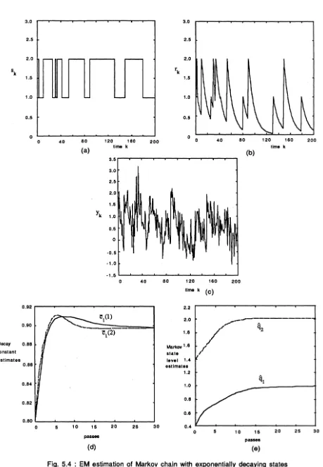
A 10000 point two-state first order Markov chain was generated with transition prob-abilities aii = 0.95, with the states qi at 1 and 2. The resulting Markov chain was expo-nentially filtered with decay constants [c1(1), c1(2)] = [0.9, 0.9] where c1(i) are defined in (5.6). Also c0(i) = 1 in (5.6). Zero mean white Gaussian noise of standard deviation

117 Fig.5.4( a), (b) and (c) show 200 points of the Markov chain Sk, the filtered chain Tk, and

the observations Yk respectively. The initial state level estimates were arbitrarily chosen as

"ih

= 0.4 and

7h

= 1.4. Also the initial decay constants were chosen as

[c

1(1),

c

1(2)) = [0.8, 0.8].

The quasi-EM algorithm was run for :30 passes on the data Yk· Fig. 5.4( d) shows the estimates of the decay constant with successive passes. Fig.5.4(e) shows the estimates of the state levels. Notice that these estimates converge to the true values. Also the transition probability estimates converge to the true values.

This and other simulations not reported here confirm that if it is apriori known that the states decay exponentially, then the EM algorithm can be used to obtain estimates of the decay constant along with the transition probabilities and state levels.

Cell Membrane data

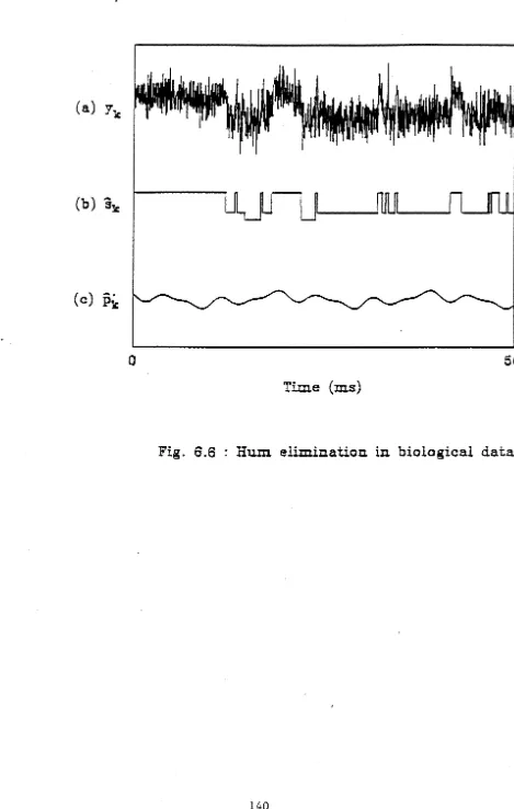
Here we describe an example of a process with exponentially decaying states. The data to model channels in cell membranes was obtained as follows: Spontaneous synaptic currents were recorded in voltage-clamped CAl cells in rat hippocampal slices at room temperature. The pyramidal neuron was impaled with a microelectrode, which was filled with 3 M KCl, and then its intracellular voltage was clamped at -60 mV with respect to the extracellular medium, using a voltage clamp amplifier. This instrument permits voltage clamping with ·one electrode which is switched at high frequency between current passing and voltage recording modes. The recorded currents, which show a rapid rise and decays back exponentially, are spontaneous inhibitory post-synaptic currents generated by the opening of chloride-selective channels activated by 1-aminobutyric acid.

500~---~---~---~

·-·--·-

·-·-·--·

--·-·

...

·-· -·-·-·

-·-·

-·-·-·

-·

-·-450 Baum-Welch

No. of errors per 1

ooo

400

points 350

300

250

\

'

\

\ \

'

_{' '}

'

,

__

....

_

'-~---

Scheme2 - .... _....

_,

---2000~--~2----~4----~6~---8~---1~0~--~12~--~1~4~~16

-7500

-7000

-6500 log L

- 6000

-5500

-5000

0

No. of passes

Scheme2

---Baum~;lch·-·-·-·-·-·-·-·-·-·-·-·-·

2 4 6 8 10 12 14

No. of passes

initial decay estimates = (0.8, 0.8, 0.8, 0.85] true decay values = [1, 0.98, 0.95, 0.95]

Fig. 5.3: Comparison of re-estimation schemes

118

[image:24.607.76.520.48.806.2]

3.0 3.0

2.5 2.5

2.0

-

-

2.0

sk rk

1.5 1.5

1.0

-

..._,

1.0

0.5 0.6

0 0

0 40 80 120 160 200

0 40 80 120 180 200

(a) time k _(b) time k

3.6

3.0

2.5

2.0

1.6

yk _1.0

0.5

0

·0.6

·1.0

·1.5

0 40 80 120 160 200

time k _(c)

0.92 2.2

~1(1) _2.0

,----1\----0.90

~/ q2

i!1 (2) 1.8

Decay 0.88 _{Markov 1.8}

constant _state ,/

estimates l level 1.4

0.86

~

estimates

1.2

I ~1

0.84 _1.0

0.8 0.82

0.8 0.80

0 5 10 15 20 26 30

5 10 16 20 25 30

passes

p - s

(d) _(e)

Fig. 5.4 : EM estimation of Markov chain with exponentially decaying states

[image:25.603.83.542.61.723.2]

a

_k

-0 100 200 300 400

lime k

Fig.S.S: Semple segments of noisy observetions, estimeted signal

end underlying Markov process of synaptic neuronal currents

121

Once the decay constants were estimated, we computed the least squares estimate of p;1,i, i = 2, 3,4. Because the rise time to a state is significantly faster than the decay, it is reasonable to expect that

J1

1,i are satisfactory estimates of the state levels of the imbedded

Markov chain. The means

J11

,i were calculated to be 49.8, 90.7, 201.4 which indeed are close to the actual states levels.

5.5

Conclusions

In this chapter schemes for estimating semi-1-farkov processes imbedded in white (or near white) noise with decaying states have been proposed. We have reformulated the Hidden semi-Markov Model problem in the scalar case as first order 2-vector, homogeneous Hidden Markov Model (HMM) problem in which the state consists of the signal augmented by the time to the last transition. With this reformulation, we have applied HMM signal processing techniques based on the forward-backward algorithm and the Baum-Welch re-estimation formulae. We also have proposed variations of the Expectation Maximization (EM) scheme for faster convergence in yielding optimal estimates of the signals and signal model parameters, including level transition probabilities and noise statistics. Finally, an example from biological signal processing of cell membrane channel currents is studied.

Appendix

Estep: This involves computing Q(.X, 'X) which is the expectation of the log of the likelihood function of the fully categorized data (see [20],

[15]

for details). Here

N N T-1 N

Q(A,'X)= L L L(k(m,n)logZimn+ L''Yl(n)log11'"n+Q2 (A1)

m=l n=l k=l n=l

where

122

O:mn and 1Fm. Now consider maximizing the third term in (Al) namely Q2: Solving for

Chapter

6

Hidden Markov Model Signal

Processing in presence of

unknown deterministic

interferences

6.1

Introduction

Hidden Markov Model (HMM) processing techniques are used to extract discrete-time finite-state Markov signals imbedded in Gaussian white noise [21], [52]. Here, motivated by examples in neuro-physical signal processing of ionic currents in cell membrane channels explored in more detail in a companion paper [6], we consider the case where in addition to Gaussian white noise, the Markov process is also corrupted by a deterministic signal of known form but unknown parameters. We consider two such examples of deterministic disturbances:·

1. Periodic or almost periodic disturbances, with time variable k, of the form

Ef=t

ai sin( Wi k+

</>;) where the frequency components w;, amplitudes a; and phases

4>i

are unknown. An example of such periodic disturbance with known frequency components (the fundamental and harmonics) is the periodic 'hum' from the electricity mains which may be too costly to eliminate from some experimental environments.

2. Drift in the set of state levels of the Markov process in the form of the polynomial

124

I:f=1

ai ki with the coefficients ai unknown. For example, such drift can occur in cell

membrane channel current measurements due to the slow development of liquid junction potentials arising from two different solutions of ionic compositions [14]. This drift can be adequately modelled by a polynomial function of time.

It might be argued that the classical problem of periodic disturbance suppression with known frequency components can be effectively solved by notch filtering or averaging meth-ods. However, traditional schemes such as notch filtering have a considerable transient response and so distort the imbedded Markov chain. Also, simulations (not presented here) show that even in low noise, heuristic methods such as averaging observations sepa-rated by multiples of the period yield unsatisfactory estimates. Variations of this method involving more complex moving average (or median) filtering to average out the noise do not appear to yield significant improvement.

More recently, in [64], a generalization of the notch filtering approach is presented for eliminating exponential interferences including sinusoids from finite-length discrete-time signals such as step responses. This scheme however, does not exploit the Markovian nature of the imbedded signal. ·Moreover, such schemes do not learn anything about the periodic disturbance. Thus there is incentive to seek optimal suppression or estimation of the deterministic disturbance. In deriving optimal schemes, all the apriori information available must be used: the nature of the deterministic disturbances ( eg. periodic or polynomial), the Markovian characteristics of the imbedded process and the presence of white Gaussian noise.

Methods for estimating a periodic signal in noise are usually highly sensitive to fre-quency uncertainty. In our experience, estimates of the frefre-quency components of the periodic disturbance obtained by a Fast Fourier Transform (FFT) on the data are not sufficiently accurate, especially in high noise. Hence the need for deriving schemes that achieve optimal frequency estimation of the periodic signal in a mixture of white noise and a finite-state Markov process.

125

case, maximum likelihood estimates of the frequency components, phases and amplitudes are obtained. The algorithms we present here are attractive because of their sound the-oretical basis and do not require undue complexity in their implementation. Further, simulation studies confirm their optimal (maximum likelihood) performance.

The chapter is organized as follows: In Section 6.2 the problem is formulated as a HMM problem. In Section 6.3, our techniques for obtaining the maximum likelihood estimates are described. Finally simulation examples are presented in Section 6.4 and conclusions in Section 6.5.

6.2

Problem Formulation

In this section, first the signal model is described and then estimation objectives are presented.

Signal Model: Consider a discrete-time finite-state homogeneous Markov process s~c.

At each time k, Sk takes on one of a finite number N of states q1, q2, ... , qN, organized as a vector q. Denote the sta.te transition probabilities as amn = P(sk+l = qnls~c = qm) and the corresponding transition probability matrix by A= (amn)·

Let p~c(0), parametrized by 0 E IRR denote a deterministic disturbance. We assume that the functional form of JJk is known but the parameter vector 0 = ( 817 ••• , 8n) is unknown. eg. in the periodic or almost periodic case, 0

= (

a17 .•• , ap, ¢>17 ... , <f>v) and Pk(0) =

L:f=1

ai sin(wi k+¢;). In the polynomial drift case, 0 =

(a1, ...

,ap) and P~c(0) =

L:f=l

ai ki.

To make a connection \vith the theory of HMMs, we assume that the Markov process

Sic is hidden, that is indirectly observed by measurements Ylc, where

Yk = Sk

+

Pk +Wk.

(6.1)

Here Wk is zero mean normally distributed Gaussian white noise of variance 0'~. We denote the sequence Yll y2 , ••• , Yk by Yk. Define the vector of probability functions b(0, 0'~, q, Ylc)

=

126

For notational convenience, in the rest of the chapter we shall denote bi(9,

0'!,

q, Yk) by

Because Wk is white, the independence property P(yk- Pklsk

=

qi, Sk-1

=

qj, Yk-1)

=

P(yk-Pklsk = qi) which is essential for formulating the problem as a HMM holds. Also we assume that the initial state probability vector 1L

=

(7ri) is defined from 11"i

=

P(s1

=

qi)·

The HMM is denoted A= (A,0,a.~,q,1[.).

Estimation Objectives: Given the above signal model, there are three inter-related HMM problems which can be solved [21], [52] and interpreted to yield results for the underlying Markov process.

1. Evaluate the likelihood of a given model Ai generating the given sequence of data, denoted P(Y kiAi)· This allows comparison of a set of models

{Ai}

to select the most likely, given the observations.

2. Estimate statistics of the signal Sk such as a posteriori probabilities for an assumed model A and data sequence. For a fixed interval T, estimate

(6.3)

From /k( m ), state sequence estimates conditioned on A, such as maximum a posteriori (MAP) can be generated as

.sMAP = q where m = arg max "'~k(i)

k m 19~N r (6.4)

3. Process the observations based on a model assumption A, and re-estimate the model parameters (functions) (A, 0,

a!,

q,K.), such that the likelihood of the observation sequence given the updated model~= (A, 0, cr~,

q,:zE)

namely P(Yti'X) is improved, i.e.,

P(Yri'X)

>

P(YriA), and repeating until convergence. The objective is to achieve the most likely model ~ML amongst the set A= (A,

e,

0'~, q,K.), given the observations.

6.3

Estimation and Re-estimation

127

6.3.1

Forward-Backward Procedure

The solution to Problems 1 and 2 involve the Forward-Backward procedure which we briefly describe now:

Consider an observation sequence Y T and assumed signal generating model .A. Forward and backward vector variables are defined as probabilities conditioned on the model .A, for m = 1, 2, ... , N as follows:

£:::.

f!k

=

(ak(m)); ak(m)

=

P(Yk,sk

=

qmi.A)

£:::.

-f!_k

=

(Jh(m)); !3k(m)

=

P(Ykisk

=

qm,.A)

where Yk denotes the future sequence Yk+l• Yk+2• ... , YT·

Recursive formulae for frk and f!_k are readily calculated [21] as

ak(n)

=

(,~

1

ak-l(m)amn) bn(Yk), a1(n)

=

1f'nbn(YI)

N

!3k( m)

=

L

amn bn(Yk+d !3k+l (n), f3r(m)

=

1

n=l

The optimal a posteriori probabilities associated with Problem 2 are given from [21] (6.5)

(6.6)

ak(m)j3k(m)

1k = (!k(m)); /k(rn) ='EN ( );3 ( )' m = 1,2, ... ,N. (6.7) m=l ak m k m

Then using (6.4) we obtain MAP fixed-interval smoothed estimates. The likelihood func-tion, which is the end result of the Problem 1, is calculated as

N

Lr

~

P(Yri.A) =

L

ar(m). (6.8)

m=l

6.3.2 EM algorithm

128

E step: This involves computing Q( A,

'X)

which is the expectation of the log of the likelihood function of the fully categorized data (see [20], [15] for details). Here

N N T-1 N

Q(A,

'X)=

I: I: I:

(k(m,n)logamn

+I:

/1(n)log1fn

+

Qz (6.9)

m=l n=l k=l n=l

where

(6.10)

(6.11) and 7in is the estimate of the Markov state level qn.

M step: This involves finding

'X

to maximize Q(A,

'X).

The optimal HMM A is loosely denoted

'X.

Maximizing the first two terms on the right hand side of (6.9) yields the standard Baum-Welch equations

[17], [18], [19]

for re-estimating 7lmn and 1fm, namely,

-

L:r::ll

(k(m,n) - ( )

amn

=

"'y_

1 "'N ( ( ); 1l"m

=

/1 n

L...k=l L...n=l k m, n

Also solving for ~g2 = 0 yields the new estimate

qn

as qn

Solving for ~g. = 0 gives

uf7w

(6.12)

(6.13)

(6.14)

We also require to solve for

7Ji

in &~? = 0 to maximize Q2 • Details are developed for

&B;

periodic and polynomial drift disturbances in the next two subsections.

6.3.3 Periodic Disturbances

To fix ideas, we first consider the case where the frequency components of the periodic (or almost periodic) disturbance are known. Later in this subsection, the more general case with unknown frequency components will be considered.

129

ai E R. Also Wi

=

211" /Ti where Ti is the period of the i th sinusoidal component.

Solving for

OJ?

= 0 yields the new estimate

(6.15)

Also, solving ~~:

=

0 yields

(6.16)

where

c1 =

L L

idn)(Yk -7jn-

Lai

sin(wj k

+

¢)j))cos(wi k)

k n j#i

c2

= -

L L

ik( n)(yk -7jn-

Lai

sin(wj k

+

¢)i))

sin( Wi k)

k n j#i

Based on (6.13), (6.14), (6.1.5) and (6.16) we now propose three methods for re-estimating

7in,

0'!,

ai

and (i)i.

!.Standard EM Re-estimation: To solve for 7jn,

0'!,

ai

and ¢)i, we need to solve (6.13), (6.14), (6.15) and (6.16) simultaneously. This is easily done (although the algebraic manipulation is tedious) as follows: From (6.15) and (6.13),

ai

and

7in

can be expressed as explicit functions of¢). Then substituting for these in (6.16), we solve for (6.16) numerically for

¢)

and so calculate 7jn,

a!

and

ai.

2.Block Component Re-estimation [67]: Here we iteratively maximize Q2 with respect to one variable at a time keeping the others constant. Thus we keep ai, </>i and

Uw constant and update qn. Then we use the updated qn, keep </>i and Uw constant and

re-estimate ai and so on. This scheme ensures that the likelihood function improves after

each pass. Thus in each pass one of the equations {6.13), (6.14), (6.15), (6.16) is used with 7in,

a!, ai

and ¢)i in the right hand sides of the equations replaced by qn, u!, ai and

</>i.

Note that the transition probabilities are updated every pass since their re-estimation equations are independent of maximizing Q2 •

130 similar to that in [65], [66]. In re-estimating qn, a~, a; and <i);, we use (6.13), (6.14), (6.15) and (6.16) with

7i.n,

a~,

a;

and¢'>; in the right hand sides of the equations replaced by

qn,

0';,

a; and

</>i.

Then because c1, c2, d1 and d2 are independent of<i);, (6.l6) is easily solved for

¢;

numerically. The simulations we present subsequently use this quasi-EM algorithm and show that the algorithm yields acceptable results.

Frequency Re-estimation:

So far we have assumed that the frequency of the components of the periodic signal are known precisely. Here we deal with the case when the frequency components are unknown.

It might seem feasible to estimate the frequency components by applying a Fast Fourier Transform (FFT) on the data. However FFTs are not very accurate especially in high noise. We show subsequently in simulation studies that the performance of the above proposed schemes rapidly degrade even with small errors in the frequency. So the FFT is not suitable for obtaining estimates of the frequency components.

We now propose a scheme for re-estimating the frequencies which is an extension of the EM scheme proposed above for estimating the amplitudes and phases.

Here because the frequency components are also unknown, the parameter vector to be estimated is

e

= ( al, ... , Clp, <1>1, ... , </>p, WI, ..• , Wp)• Again we maximize

(;.h

defined

in (6.10) with w; in Q2 now replaced by w;. Setting the derivatives of Q2 with respect to

qn,

a~,

a;

and

¢;

to zero yield (6.13), (6.14), (6.15) and (6.16) respectively. Setting

8Q2/

Ow;

= 0 yields

T

fi(w)

~

L

hk cos( w; k+<i);)-a; k sin(2( w; k+¢'>;))-k

L

ai sin( Wj k+<i)j) cos(wi k+<i);)

=

0.

k=l j:j:i

(6.17) where hk

=

k(Yk-

I:;;=

I /k( n) 7in) and w

=

(WI. ... ,

wpf·

Equation (6.17) has numerous solutions. The solution which we choose to yield a maximum likelihood estimate is that which maximizes Q2. Of course if intervals in which the various frequency components occur are apriori known (these intervals can be found from a FFT), then only the solutions to (6.17) belonging to these intervals need to be considered.

131 F(w) = (h(W), ... , /p(w). Then the Newton Raphson update equation is

(6.18)

where G

=

(g;j), 9ij

=

&Ji/Dwj. So

9ii

= -

2::

k hk sin( w; k

+

~;)

-

a;k2 _{cos(2(w; k}

+

_'¢;))

+

_k2

2::

_{lij sin( Wj k}

+

_{'?)j) sin(wi k}

+

_'¢>;)

k j~i

9ij = -aiLk2cos(w;k+~;)cos(wjk+'¢>j) (6.19) k

Remark 1: In the implementation of the above scheme, it is necessary to store the T

scalars, hk, k = 1, ... , T. So the memory requirements here, (N

+

1)T, are only slighly more than that for standard HMM processing (NT).

Remark 2: Any one of the EM, quasi-EM or Block Component Re-estimation can be used.

Remark 3: Equation ( 6.17) is rather illcondi tioned. However, as demonstrated in

simula-tions subsequently, double precision arithmetic appears adequate for its numerical solution.

0

6.3.4 Drift

L L

'i'k( n )(Yk-qn)k;

=

2::

Pk(e) ki, i

=

1, ... ,p (6.20)

k n k

Solving these p equations which are linear in a; yield a;. Again any one of the EM, quasi-EM or Block Component Re-estimation schemes can be used.

6.4 Simulation

Studies

We illustrate the performance of the proposed algorithms for periodic disturbances and polynomial drift.

6.4.1

Periodic Signals

(a)

~ ~

[

Ul

uu

fL

(b) Yk

(c)

Be

(d)

~ ~

[

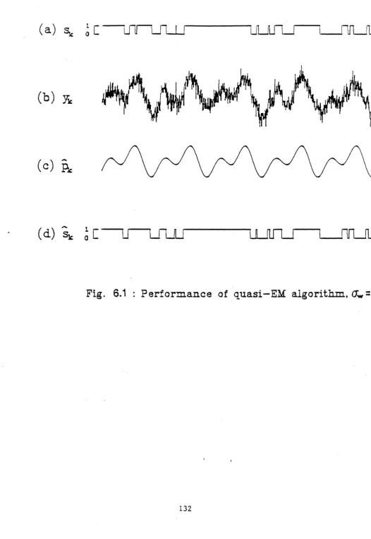
Fig. 6.1 : Performance of, quasi-EM. algorithm,

fJw

=

0·5

[image:38.605.33.559.48.811.2]

133 Example 1 (Medium noise): The purpose of this simulation example is to show that the proposed algorithms satisfactorily learn the Markov state levels, state estimates and transition probabilities, and also amplitude and phase of the components of the periodic signal (with known frequency components) from the sum of the Markov signal, periodic signal and Gaussian white noise with known variance.

A 20,000-point 2 state discrete-time Markov chain was generated with transition prob-abilities aii

=

0.97, aij

=

0.03. The state levels of the Markov process were q1

=

0 and

q2 = 1. To this chain was added zero-mean white Gaussian noise of known standard devi-ation CTw = 0.5. Also a periodic signal Pk = a

₁

sin(2 7rk/200

+

</>t)

+

a2 sin(211'k/100

+

¢>2) was added with 0 = (at. az, ¢;, ¢2 ) = ( 0.8, 0.8, 0, 0). The initial Markov state level esti-mates were taken as

7h

=

1..5, 7]2

=

2 .. 5. Also the initial estimate 0 = (0.75,0.75,0.50.5) and "ilii = 0.95. Fig.6.1a and 6.lb show a 1000-point sample of the Markov chain and observations (obtained by adding the 1Iarkov chain, periodic signal and white noise).

After 500 passes,

7lt

= -0.011 and 7]2 = 0.997 and "ilu = "il22

=

0.969. Also after 500 passes 0

=

(1.002, 0.994, 3.95 x 10-3_{,2.22 x 10-}6 ). Using these values of 0 we plotted 1000 points of the estimated periodic signal Pk in Fig.6.1c. In the scale of Fig.6.1, the plots of Pk and Pk are identical. Finally, Fig.6.1d shows the corresponding 1000 points of the estimated Markov signal

St..

Here l\TAP estimates (see (6.4)) were used.

The plots in Fig.6.1 show that the proposed scheme perform adequately in a 'medium' noise environment.

Example 2 (High noise): This simulation example shows that the proposed algorithms perform satisfactorily even when the Gaussian noise has a large known variance.

To the Markov chain in Example 1 was added zero-mean white Gaussian noise of known standard deviation CTw

=

4. Also a periodic signal Pk = a1 sin(211'k/200

+¢>I)+

a2 sin(211'k/100

+

¢>2) was added where 0

=

(al,a2,¢>i,¢>2)

=

(0.8,0.8,7r/4,0). Fig.6.2a shows a 1000-point sample of the ?\Iarkov chain, Fig.6.2b shows the periodic signal and Fig.6.2c shows the observations obtained by adding the Markov chain, periodic signal and white Gaussian noise.

0

500

1000

[image:40.620.58.560.61.742.2]

Time k

...

Initial

est~ate

(d)

···--··-

lst pass

·---

2nd pass

rs:

1

pk

....

0

O'l

Ql

0

.,!

!d

e

·-....

_Time

O'l 1:1

-1

__

...

Fig.

6.2:

Performance of Quasi-EM algorithm,

CJw

=

4