Int. J. Electrochem. Sci., 10 (2015) 5130 - 5151
International Journal of
ELECTROCHEMICAL
SCIENCE
www.electrochemsci.org
Lithium-ion Battery Security Guaranteeing Method Study
Based on the State of Charge Estimation
Shunli Wang1,*,Liping Shang1,Zhanfeng Li2, HuDeng1,Youliang Ma2
1
School of Information Engineering & Robot Technology Used for Special Environment Key Laboratory of Sichuan Province, Southwest University of Science and Technology, Mianyang 621010, China
2
School of Manufacturing Science and Engineering, Southwest University of Science and Technology, Mianyang 621010, China
*
E-mail: [email protected]
Foundation item: Sichuan Science and Technology Support Program (2014GZ0078), Laboratory Open Fund (14xnkf09).
Received: 2 March 2015 / Accepted: 6 April 2015 / Published: 28 April 2015
[Purpose] The security guaranteeing method for the lithium-ion battery is studied and a novel state of charge (SOC) estimation method is proposed based on the Kalman filtering (KF) thought, aiming to guarantee its safety in the power supply application of electric vehicles (EVs). In this study, there are several parts that have been studied to realize the protection of the lithium-ion battery during its whole life period. Firstly, the core parameters for the working state estimation of the lithium-ion battery is studied and the methods for the state of charge estimation are analyzed. Secondly, the working state of the lithium-ion battery is estimated by the integrated application of the state of charge estimation methods. Then, the estimation model is designed and realized based on the estimation principle. At last, this method and model is proved by the experimental analysis. In the experiments, the main operating temperature varies between 26.84 ℃ and 33.16 ℃, with an average value of 30 ℃. The average value of the Coulomb efficiency is about 0.97 and all above 0.95. The average value of the battery capacity is approximately 45.08Ah. When the SOC actual initial value is 0.8 and the test initial forecast value is 0.6, the estimation can track the actual value in less than 5 seconds and has high accuracy. The error covariance value is smaller than 3.5×10⁻⁶
and decreases rapidly as time goes. This study can achieve the working state estimation of the lithium-ion battery, which can guarantee its safety effectively in the power supply applications.
1. INTRODUCTION
Because of the oil and energy shortages and the air pollution, the development of energy-saving electric vehicles (EVs) has become one of the major energy supply development trends in the automotive industry [1-3].
Energy is an important material foundation for the economic growth and social development. And in the application course of energy, it has caused environmental pollution, climate change and other serious problems [4-5]. Whether the energy consumption and emissions in the transport sector and other issues can be effectively resolved will directly affect our social development. Aiming to solve these problems, many countries are promoting the development of EVs industry vigorously [6]. The batteries which is used as the main power source of EVs are required to have high specific energy, high specific power and high charging and discharging efficiency [7-12]. Lithium-ion batteries (LIBs), because of its high energy density, high voltage, long cycle life, safety, reliability and other good characteristic features, are becoming one of the major power sources for EVs [13].
The state of charge (SOC) of the LIBs is an important core parameter in the application of batteries, requiring the accurate measurement of the equation parameters in the development of EVs, which is becoming a very critical issue [14-18]. Only with accurate measurement equations of the SOC, it is able to manage the battery energy effectively to prevent it from charging or over-discharging risks [19]. It can provide the necessary data basis for other energy related system programs as well. However, the present estimating technology is not capable for the accurate real-time measurement of SOC [20-23]. As a result, we can only think of other approaches to improve the SOC estimating accuracy. In the process of the SOC value estimation, we must consider the impact of various factors in the LIBs working process, using reasonable equivalent circuit model of the LIBs [24-32]. The appropriate estimation algorithms are used to improve the accuracy of the SOC estimation.
The batteries and battery management systems (BMS) are the key components of EVs [33-39]. The SOC value, which marks the power remaining of the batteries, is also the core parameter of the BMS. It is a reflection of the operational status of the main parameter, providing a basis for the vehicle control strategy judgment and management. And the accurate estimation and management of SOC can improve the battery sate of life (SOL) and the vehicle application performance.
2. MATHEMATICAL MODEL ANALYSIS
2.1. SOC definition
The battery SOC is used to reflect the status of the battery remaining capacity. The SOC value cannot be obtained directly from the direct detection of the battery parameters (especially for the real-time working state monitoring), but only by measuring the outer characteristic parameters of the battery packs and estimating indirectly. It is defined on the ratio value of the residual capacity and the representing rated capacity as shown in Eq.1.
100%
c
I
Q SOC
C
(1)
Where, Qc is the remaining capacity of the battery and CI is the rated capacity, in which the battery discharges at the constant current I and gains its capacity by multiplying current with the discharging time in hours.
The SOC is defined as the ratio between the saved energy in a battery and the whole energy that could be saved in it by Shahriari et al [22] which verify this definition. Because the capacity of LIBs varies along with the discharging current greatly, it is necessary to signal the discharging current when the capacity value is used.
In the actual EVs application, the battery SOC estimation formula to define the working sate is quite complicated. The reason is that, in the battery SOC estimation process, it is necessary to fully consider the current, voltage, self-recovery, temperature, charging or discharging rate, cycle numbers, aging degree and other factors which have great impacts on the battery SOC estimation.
2.2. Battery impact factor analysis and demonstration
In the SOC estimation process of LIBs in the EVs application, the SOC value of the battery is related to the discharging current, monomer temperature, battery remaining life, self-discharging rate and other factors. The number of recycling is especially exhibiting a high non-linear degree, which brings a lot of difficulties to the accurate SOC value estimation.
2.2.1. Battery temperature
electrochemical reaction will be inhibited, the actual usable capacity of the battery will be reduced, and the energy utilization efficiency will decline, as a result, the maximum allowable discharging current is reduced. When the temperature rises, the actual battery capacity will increase, but when the temperature is too high, the battery capacity and charging-discharging efficiency will decline as well. Therefore, the actual capacity of the lithium-ion battery will experience a non-linear change along with the variety of the operating temperature. Therefore, the operating temperature of the factors cannot be ignored for the LIBs SOC estimation.
2.2.2. Charging-discharging rate
The discharging currents in the operating process inevitably exhibit a considerable nonlinearity. The LIB electricity release varies at different discharging currents. When the LIB discharges with a large discharging current, the total power release of the battery is quite small. While with a smaller discharging current, the total current release will increase. Therefore, in the SOC estimation process, we must consider the discharging current or current rate as an important factor.
2.2.3. Self-discharge
During the storage period of the battery, due to the impurities inside the battery, the battery positive and negative electrode active material is gradually consumed, resulting in the loss of battery capacity. This phenomenon is called self-discharge of the battery. The higher temperature and humidity will accelerate the battery self-discharge reaction. After a period of time that the battery is allowed to stand, the battery power is stabilized. However, if after a longer standing, the battery will slowly lose power, namely the phenomenon of self-discharge. Because KF algorithm is used in this study and the algorithm itself has a self-correcting function, this factor can be ignored.
2.2.4. Battery Life
The charging-discharging cycle means undergoing a whole battery charging and discharging process. Under certain discharging conditions prior to the specified battery capacity, the battery can withstand the number of cycles which is called cycle life. With the reduction of the battery life, the battery capacity will be reduced accordingly, which is related to the remaining discharging capacity directly. When the remaining battery power is low, the Coulomb effect will reduce. Therefore, the battery life also affects the SOC estimation for LIBs.
2.3. SOC estimation Methods
voltage) method, linear model method, resistance reckon method, KF method, neural network method and so on.
2.3.1. Discharging experimental method
In the discharging experimental method estimation process, the constant current discharging experiments are done for a sustaining discharge, in which the release capacity of electricity is obtained by multiplying the discharging current with time. This method is more accurate compared with other SOC estimating methods, but this charging and discharging test need too much experimental time, calculating this method cannot be used in the working environment of the LIBs. It is commonly used in the offline calibration of the battery capacity.
2.3.2. Ah estimation method
Ah method for SOC estimation is one of the most commonly used methods for estimating the SOC value and is the theoretical basis of other commonly used methods. The principle is that the battery is calculated by using the cumulative release of electricity in a certain time to estimate the SOC value with the time parametert. The SOC calculation process is shown in Eq.2.
0 0
1
( ) t
n
SOC t SOC I d
Q
(2)Wherein, SOC0 is the initial residual capacity; Qn is the battery rated capacity; I is current for
time charging and discharging process, the value of which is positive when doing discharging maintenance and negative in the charging maintenance process; is the Coulomb effect.
As we can know from this SOC value estimating principle, it is quite a simple method to calculate the SOC value by using the Ah estimation method, but due to the imprecision of the current measurement accuracy in the charging and discharging maintenance process, the SOC value cannot be obtained very precisely only by using this equation and there are always some inevitable cumulative errors. However, it has strong adaptability and is available for all material type batteries.
2.3.3. OCV method
2.3.4. Linear model method
The principle of linear model method is realized by considering the SOC value at thek1 time point, i.e., SOCk1, the current voltage U k
and the current I k are also used in this method to establish a linear equation, thereby obtaining the operating SOC value of the battery, i.e.,SOCk. The linear model method estimating equation is shown in Eq.3.
0 1 2 3 1
1
k k
k k k
SOC U k I k SOC
SOC SOC SOC
(3)
Wherein, the0,1, 2, 3 are the model parameters which can be obtained by using the
MATLAB curve fitting method. As mentioned above, this model is quite simple while the accuracy of this method is not high in the SOC value estimating process. As a result, this method is used only in the rough estimating process.
2.3.5. Internal resistance method
The internal resistance method is realized by using external power excitation, in which a different frequency alternating current is used to trigger the battery excitation and the measurement of equation AC resistance inside the battery is done simultaneously, and the calculation model is also used to obtain the estimated SOC value as well. Theelectrical equivalent circuit model is also used as one of the most important parameters for the SOC estimation in KF and neural network methods [17]. However, the internal resistance and the SOC value are both closely related to temperature and the battery large extent aging effects. What’s more, the measurement for these experimental parameters is very difficult. As a result, the method is rarely used in EVs application environments.
2.3.6. KF method
The KF method is based on the law of Ah integration method, which is also a recursive estimating method. It only needs to know the status of the measured values, covariance on the time value, the covariance of the current state at present for calculating the SOC value. It can be calculated to estimate of the SOC state accurately and their estimation errors can also be obtained at the same time. Therefore, this SOC estimation method has better accuracy and timeliness for a variety of EVs battery, which experiences intense current fluctuations relatively. However, this method depends on the large matrix operations which require higher computing power processor.
2.3.7. Neural network method
Because the KF is based on the analysis of these above estimation methods and considering the battery temperature, charging or discharging current, remaining capacity, internal resistance, etc., the KF algorithm simulation model is more suitable for EVs and the LIBs working conditions, which can be realized with good accuracy.
2.4. KF estimation principle
The KF estimation is realized by using the recursive calculation thought in the estimating process. It can gain good experimental results to realize the SOC state estimation in the LIBs management system and the parameter identification. Its principle diagram is shown in Fig.1.
B
k + DelayC
k +D
kA
kXk+1 Xk
vk
wk
yk
[image:7.596.204.391.279.358.2]uk
Figure 1. KF estimation principle
The KF estimation structure can be obtained by the discrete state equation and measurement equation as shown in Eq.4.
1
1
k k k k k k
k k k k k k
x A x B u w
y C x D u v
(4)
Wherein, the parameters of xk and xk1 respectively represent the intermediate variable values at the time points of tk and tk1; The parameter uk indicates the system input;Ak, Bk, Ck,Dk are respectively the system state matrix, control matrix, measurement matrix and the input-output relationship matrix; wk indicates the process noise, which meets the zero mathematical expectation. The covariance matrix of Qkhas the multivariate normal distribution, the relationship of which can be shown as wk ~N
0,Qk
; vk is used as the measuring noise, and its mathematical expectation is zero. The association covariance matrix is abbreviated asRk, and the relationship of them iswk ~N
0,Rk
; the parameters of ykand yk1 respectively represent observable equations at tk and tk1 time points.
As a result, it is just necessary to know the SOC value and the predicted covariance value of LIBs at the time point of k, combined with the time of the observations and k covariance. And then, the best estimate of the SOC value at k moment can be obtained. This method demands the high accuracy of SOC value at k1 time moment and can be done with very good convergence. Then, it can be known that the method described above uses the predicted values and observed values simultaneously.
2.5. State equation and measurement equation
In order to predict the performance of the LIBs, mounts of related research workers have established a number of different battery equivalent models. However, it is still not suitable to fully and accurately predict cell performance with just one of these models, since the model built for SOC estimation does not involve all the influencing factors for the LIBs cell performance. The simplest model is a unique model distinguished with the electrochemical theory-based analysis models. Such models can predict the energy storage capacity of the LIBs. In this paper, there are three models that are used for the representative advantages, as shown in Eq.5, Eq.6 and Eq.7 respectively.
Shepherd Model:
0 /
k k i k
y E Ri K x (5) Unnewehr Universal Model:
0
k k i k
y E Ri K x (6) Nernst model:
0 1ln 2ln 1k k k k
y E Ri K x K x (7)
Wherein, yk indicates the terminal voltage of the LIBs; Ki indicates the polarization resistance; E0 indicates the initial terminal voltage of the battery pack; Ris the internal resistance of the LIBs.
In order to ensure the better accuracy for the SOC estimation, the combined architecture of these three models is used here as one comprehensive model to establish its output equation as shown in Eq.8.
0 1/ 2 3ln 4ln 1
k k k k k k k
y E Ri K x K x K x K x v (8)
Wherein, yk indicates the terminal voltage of LIBs; K ii
1, 2,3, 4
and its parameter R is calculated by minimizing the variance principle.Because the sample data is obtained based on the sampling theorem detection in the data analysis process, we analyze the data by this analysis method requiring the use of discrete form analysis methods. As a result, the discrete formula of Eq.2 is built as shown in Eq.9.
1 /
k k n k
x x t Q i (9)
Considering the detection error, we can obtain the improved formula as shown in Eq.10.
1 /
k k n k k
x x t Q i w (10)
At this point, we can get the principle of the KF by using the state equation and the measurement equation. The Eq.10 is used as the measurement equation, and the Eq.8 is used as the state equation. The covariance is obtained by using the parameters Qk andRk. By comparing the Eq.10, Eq.8 and Eq.4, we can get the relationship of the parameters as shown in Eq.11.
1, /
k k n
A B t Q (11)
By analyzing the Eq.8, we can get the Ck value as shown in Eq.12.
1
3 4| 1 2 2
| 1 | 1
| 1 1
k k k k k
k k k k k k k
y K K K
C x x K
x x x x
(12)
Wherein, xk k| 1 represents the value we can get from the state value xk1 , obtaining the value at the time of k moment by the prediction of the k1 time point state.
Then, we can use the KF method to estimate the SOC value, the calculation process of which is shown as following.
(1) SOC value initialization
It is necessary to obtain the initial value of SOC and its error covariance by other means. The initial value of SOC in this paper is assigned as shown in Eq.13.
0 0.8, 0 var 0 1
SOC P SOC (13)
(2) Error covariance forecast
Because of the requirement of the convergence conditions, the next step of this estimation is to state the value of its error covariance forecast, which is shown in Eq.14.
| 1 1| 1
| 1 1 1| 1 1 / k k k k n k
T T k k k k k k W
x x t Q i
P A P A D
(14)
The matrixes in this model are all in one orders, i.e. the value is assigned as Ak 1, as a
result,Pk k|1Pk 1|k 1DW, in Which the DW is used as the process noise covariance and its value in this
paper is initialized as DW 0.5. (3) KF gain process
The KF gain process is shown as Eq.15, in which the parameters in Eq.11 and Eq.12 are used to predict the variable value of the next time point.
| 1 | 1 / | 1
T T
k k k k k k k k k v
x P C C P C D (15)
Wherein, Dv is for measurement noise covariance, the value of which used in this paper isDv 1.
(4) The optimal estimate of the SOC value
Considering the influences of the parameter of Y, the xk k| value can be obtained by using the Eq.16 shown as following.
| | 1 | 1
k k k k k k k k
x x K Y Y (16)
Then, it is necessary to determine the coefficients of the state equation and the measurement equation to estimate the optimal value of the SOC, by which the KF method can achieve up.
simulate the actual discharging capacity by calculating the current of the EVs. By analyzing the FUDS cycle test data, the model parameters of the battery pack can be estimated using the least squares (LS) method, the Coulomb effects η and battery capacity Qn correction factors. So far, it has been realized in the battery SOC value estimation by using the KF theory method.
3. ANALYSIS MODEL DESIGN AND IMPLEMENTATION
The overall design diagram of the analysis model is shown in Fig.2, in which we can see lots of important core parameter calibrations and signal inputs. Through the first charging and discharging module simulation of working conditions, it is necessary to calibrate the module integration method for estimating the SOC value. The load voltage is detected in the module and a preliminary estimate of the signal is infibulated into the battery SOC value estimation. The SOC value is corrected by the KF correction module to obtain accurate estimates.
Discharge experiment simulated conditions
Battery model
Output parameters Impact factor
correction
Kalman estimate correction
Error analysis HPPC/FUDS
Current
Kalman estimate correction
Capacity correction
Cn
K
SOCK
YK
SOC
Figure 2. The overall design
[image:10.596.145.443.340.723.2] [image:10.596.145.452.343.466.2]
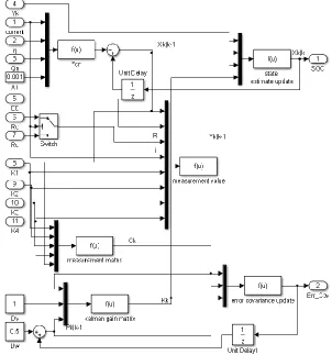
Because this estimation method is quite complicated, the estimation process is decomposed into a plurality of sub-modules. The dual Kalman filter is designed by Mastali [33] which has parameter and state measurement update. Aiming to get a fully estimation structure, the overall estimation model is designed and realized as shown in the above figure. Based on the frame structure design, the overall structure of the total analysis model diagram is realized as shown in Fig.3.
The realization of the core parts in the estimation model is designed and realized, which is shown as following.
3.1. Input Module Design
The KF algorithm is used in this paper to realize the SOC value estimation, and only the input variables of the LIBs charging and discharging current, combined with the battery operating temperature are designed here to obtain the changing law in the estimation process.
3.1.1. Current Module
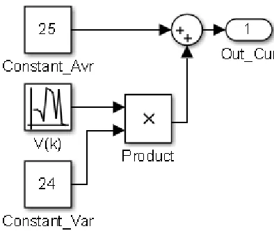
When the electrons are traveling in stable output current fluctuations around a certain value, the output current is in line with a normal distribution. In this study, the output current of the main battery pack changes from 1A to 49A and the average value is 25A, with the variance of 242, the current model of which is shown in Fig.4.
Figure 4. Current model simulation for EVs operating
Wherein, V k
subjects to the standard normal distribution. [image:11.596.196.393.435.601.2]
Figure 5. Output current waveform of the LIBs
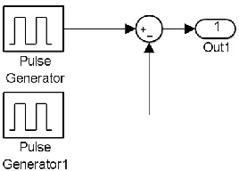
[image:12.596.158.436.70.220.2]Li-ion battery discharge curve is obtained by Orchard [32] which show the uncertain nature of the discharge profile when using the battery on a mobile mechanical system. Although the current has different ranges, there is a similar variation. In order to verify the accuracy of this model at the charging time, it is useful to set the constant current charging and discharging test module, which is shown in Fig.6.
Figure 6. Constant charging and discharging current module
The output current waveform is shown in Fig.7. The relationship between the current and the SOC is obtained by Hung (as shown in Fig. 4) [27], supporting this input current simulation.
[image:12.596.233.367.387.483.2] [image:12.596.181.417.603.717.2]
3.1.2. Temperature Module
The EVs are traveling in a stable operating temperature fluctuation around a certain value, in line with a normal distribution. The temperature-checking process is done by Kim et al [14]. Referring to this result, the main operating temperature varies between 26.84 ℃ and 33.16 ℃, with an average value of 30 ℃ in this paper. Taken 10 ℃ as variance, the temperature model is designed as shown in Fig.8.
Figure 8. Simulation model of battery operating temperature
Wherein, V k
is incited with mean value 0 and variance value 10. The output waveform of battery temperature is shown in Fig.9.Figure 9. Temperature module output waveform
In this way, the input parameters are obtained and initialized for the inputs of the SOC estimation in the KF estimation process.
3.2. Coulomb effect correction module
Figure 10. Coulomb effect correction model
The corrected Coulomb effect isK Kt SOC', wherein, the temperature correction coefficient isKt; KSOC indicates the remaining capacity correction coefficient, ' is used for the uncorrected Coulomb effect, which can be obtained by FUDS cycle test.
3.3. Battery capacity correction module
Here, it is only necessary to consider the impact of temperature on the actual battery capacity. The battery capacity is 45Ah and battery capacity correction model is shown in Fig.11.
Figure 11. Battery capacity correction model
3.4. Battery model parameter module
Figure 12. Battery model parameter module
Wherein, Rd is used as discharging resistance, and Rc is used as charging resistance.
3.5. Battery terminal voltage measurement module
This module is worth the time of SOC by k to measure the battery terminal voltage value at k moment, the model of which is shown in Fig.13.
Wherein, V k
is the measurement noise and its covariance value isDv.3.6. KF estimation module
This module implements the use of predictive value at k time point, namely, SOCk k| 1 and its error covariance measurement valueyk at the time point k . Its error covariance can be obtained as the best estimated SOC value and its error covariance can also be obtained by using the recursive filtering method. Wherein, the computing equation is introduced as shown in Fig.14.
Figure 14. SOC value estimation module using KF method
By using this module, the SOC value and its error covariance value can be obtained and used in the following modules.
3.7. Prediction module not considering various factors
[image:16.596.147.449.253.576.2]
Figure 15. Prediction module not considering various factors
Among them, the parameter K can be obtained as shown in Eq.17. 5
/ n 0.001/ 45 2.22 10
K t Q (17)
By these calculation processes, the SOC value of the LIBs can be calculated. Then, the simulation experimental test is done to prove its accuracy and reliability.
4. EXPERIMENTAL ANALYSIS
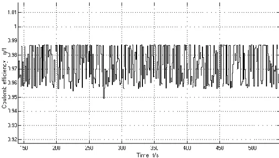
4.1. Coulomb efficiency changes in FUDS conditions
The coulomb efficiency changes in FUDS conditions are shown in Fig.16.
Figure 16. Coulomb efficiency changes in FUDS conditions
As we can see from the waveform, the average value of the Coulomb efficiency is about 0.97 and all above 0.95. If the model needs less precision or battery status is relatively stable, the Coulomb effect can also be used directly with the value of 1.
4.2. Battery capacity changes in FUDS conditions
[image:17.596.153.441.389.552.2]
Figure 17. Battery capacity changes in FUDS conditions
It can be seen from the Fig.17 that the capacity waveform varies in the entire discharging process, but the battery capacity changes very little. The average value of the battery capacity is approximately 45.08Ah. If the model accuracy is not required, or if the battery is more stable in the working conditions, the battery capacity can also be used directly rating as 45Ah.
4.3. Battery terminal voltage in FUDS conditions
The battery terminal voltage assessment results in FUDS conditions are shown in Fig.18.
Figure 18. Battery terminal voltage in FUDS conditions
experimental result is consistent with the simulation result and has the same variation which can provide the reliable input parameters for the SOC estimation model.
4.4. LIBs SOC value variation
The ideal SOC variation and experimental variation for the LIBs are shown in Fig.19. The dashed line is the estimated value of SOC and the solid line is the ideal value variation of SOC.
Figure 19. SOC estimation for LIBs in FUDS conditions
In the experiment, when the SOC actual initial value is 0.8 and the test initial forecast value is 0.6, the estimation can track the actual value inless than 5 seconds as can be seen from the waveform. the SOC value quick converge model output is close to the true value and has high accuracy. Yong Tian et al obtained the voltage profile (Fig.6) and SOC estimation results (Fig.8) by doing the equivalent circuit experiments under FUDS [4], which is consistent with the SOC estimation result using this KF estimation method. This method considers the variation of the initial state, and therefore is closer to the actual application. Since in this model the true value of the input is analog and the actual input has errors, the actual ratio of the SOC estimation error is FIG (Floated Integrating Gyro) greater. Thus, this model has good estimation accuracy and is suitable for LIBs SOC estimates in EVs.
4.5. SOC estimates not considering the various factors
Figure 20. SOC estimates not considering the various factors
Wherein, the actual initial values and prediction values are set to 0.8. The errors can be found in the waveform without considering all the factors for the SOC value estimating process, during which the discharging current is gradually increased. As we can see, if the discharging current has relatively large fluctuations, the SOC value estimating error will be greater. The cumulative SOC variation (Fig.4) is obtained by Truchot et al. [11], in which the variation law is almost the same as the estimation result by using the KF method. Because of the influence the starting state of the battery, the initial SOC value is a little different, starting from 1.0, but having the same vitiating law .
4.6. Error covariance analysis for SOC estimates
The error covariance for the SOC estimating experimental results are shown in Fig.21.
Wherein, the EC (error covariance) value is smaller than 3.5×10⁻⁶
and decreases rapidly as time goes as can be seen in Fig.21. The waveform shows that the estimation results have good convergence in the LIBs charging and discharging maintenance process.
5. CONCLUSION
In summary, the combined SOC value estimation model based on the KF estimation principle of LIBs has good accuracy and is suitable for SOC estimate of LIBs in the EVs application and working conditions.
The SOC state is a very important part of the EVs energy management system and has an important impact on the energy management system, which is designed to achieve its energy management functions and realizes battery security guaranteeing. The KF method is used to estimate the SOC value in varies working conditions, with very good accuracy at the time of steady driving EVs. The method has a smaller amount of calculation that can be applied directly for the existing battery management system hardware, without the need of raising the hardware standards. However, this method does not consider the inconsistencies and complicated road of the LIBs between the monomers and their influence on the accurate estimation of SOC value, which requires further improvement.
The design of this actual SOC value estimation model for the LIBs is closely related to human life, energy supply, and environmental issues. It is just a starting point to study the SOC estimation modeling based on the MATLAB-based analysis of recycled automotive LIBs - lithium iron phosphate battery (LiFePO4). Firstly, a lot of literature data is analyzed for the LIBs working conditions, and the
battery SOC definition is definitude. Then, the battery equivalent model and the common factor in the estimating process of the battery SOC and variety of estimation methods, establishing the design of the battery SOC estimation algorithm - KF algorithm. Hereafter, the combined battery equivalent model based on the principles established in accordance with the KF model to estimate the battery SOC value, which is established by the response of the circuit simulation in MATLAB. At last, the experimental analysis is done, in which both of the HPPS and FUDS conditions are verified. The resulting data is analyzed in order to prove that the model has high accuracy, good adaptability, strong convergence, etc. The results show that it fully meets the expectation of LIBs in the EVs working conditions.
References
1. J. Cannarella, C.B. Arnold, J. Power Sources, 269 (2014): 7-14.
2. B. Pattipati, B. Balasingam, G.V. Avvari, J. Power Sources, 269 (2014): 317-33. 3. L.P. Shang, S.L. Wang, Z.F. Li, Int. J. Electrochem. Sc., 9 (2014) (11): 6213-24. 4. Y. Tian, C.R. Chen, B.Z. Xia, Energies, 7 (2014) (9): 5995-6012.
5. C. Fleischer, W. Waag, H.M. Heyn, J. Power Sources, 260 (2014): 276-91. 6. X.S. Hu, R. Xiong, B. Egardt, IEEE T. Ind. Inform., 10 (2014) (3): 1948-59.
9. S. Sepasi, R. Ghorbani, B.Y. Liaw, J. Power Sources, 255 (2014): 368-76. 10. L.S. Wu, H.C. Chen, S.R. Chou, Energies, 7 (2014) (5): 3438-52.
11. C. Truchot, M. Dubarry, B.Y. Liaw, Appl. Energ., 119 (2014): 218-27. 12. Y.J. Xing, W. He, M. Pechtb, Appl. Energ., 113 (2014): 106–15. 13. S.S.Y. Ng, Y.J. Xing, K.L. Tsui, Appl. Energ., 118 (2014): 114-23. 14. J. Kim, S. Lee, B. Cho, J. Power Electron., 12 (2012) 1.
15. D. Andre, C. Appel, T. Soczka-Guth, J. Power Sources, 224 (2013) 20. 16. C. Hu, G. Jain, P. Tamirisa, Appl. Energ., 126 (2014) 182.
17. D. Andre, A. Nuhic, T. Soczka-Guth, Eng. Appl. Artif. Intel., 26 (2013) 951. 18. C. Fleischer, W. Waag, Z. Bai, J. Power Electron., 13 (2013) 516.
19. M. Gholizadeh, F.R. Salmasi, IEEE T. Ind. Electron., 61 (2013) 1335. 20. J. Kim, S. Lee, B.H. Cho, IEEE T. Ind. Electron., 27 (2012) 436. 21. W. Waag, D.U. Sauer, Appl. Energ., 111 (2013) 416.
22. M. Shahriari, M. Farrokhi. IEEE T. Ind. Electron., 60 (2013) 191. 23. A. Eddahech, O. Briat, N. Bertrand, Int. J. Elec. Power., 42 (2012) 487. 24. C. Hu, G. Jain, P.Q. Zhang, Appl. Energ., 129 (2014) 49.
25. J. Cannarella, C.B. Arnold, J. Power Sources, 269 (2014) 7.
26. S. Donghwa, M. Poncino, E. Macii, IEEE T. Comput. Aid. D., 34 (2015) 252. 27. M.H. Hung, C.H. Lin, L.C. Lee, J. Power Sources, 268 (2014) 861.
28. J. Kim, B.H. Cho, J. Power Sources, 260 (2014) 115. 29. X.B. Han, M.G. Ouyang, L.G. Lu, Energies, 7 (2014) 4895. 30. J.B. Yu, IEEE T. Instrum. Meas., 63 (2014) 1709.
31. J. Xu, C.C. Mi, B.G. Cao, IEEE T. Veh. Technol., 63 (2014) 1614.
32. M.E. Orchard, P. Hevia-Koch, B. Zhang, IEEE T. Ind. Electron., 60 (2013) 5260. 33. M. Mastali, J. Vazquez-Arenas, R. Fraser, J. Power Sources, 239 (2013) 294. 34. S. Schwunk, N. Armbruster, S. Straub, J. Power Sources, 239 (2013) 705. 35. C. Fleischer, W. Waag, Z. Bai, J. Power Electron., 13 (2013) 516.
36. Z.Q. Chen, L.Y. Wang, G. Yin, IEEE T. Energy. Conver., 28 (2013) 860.
37. C.A.A. Juan, J.G.N. Paulino, B.V. Cecilio, IEEE T. Power Electr., 28 (2013) 5919. 38. L. Wang, J.S. Zhao, X.M. He, Int. J. Electrochem. Sc., 7 (2012) 345.
39. J. Xu, B.G. Cao, Z. Chen, Int. J. Elec. Power., 63 (2014) 178. 40. M. Corno, N. Bhatt, IEEE T. Contr. Syst. T., 23 (2015) 117. 41. Y.J. Xing, W. He, M. Pecht, Appl. Energ., 113 (2014) 106.