This is a repository copy of
Efficient simulation of chromatographic separation processes
.
White Rose Research Online URL for this paper:
http://eprints.whiterose.ac.uk/125592/
Version: Accepted Version
Article:
Brown, S.F., Ogden, M.D. and Fraga, E.S. (2018) Efficient simulation of chromatographic
separation processes. Computers and Chemical Engineering, 110. pp. 69-77. ISSN
0098-1354
https://doi.org/10.1016/j.compchemeng.2017.12.006
Reuse
This article is distributed under the terms of the Creative Commons Attribution-NonCommercial-NoDerivs (CC BY-NC-ND) licence. This licence only allows you to download this work and share it with others as long as you credit the authors, but you can’t change the article in any way or use it commercially. More
information and the full terms of the licence here: https://creativecommons.org/licenses/
Takedown
If you consider content in White Rose Research Online to be in breach of UK law, please notify us by
Efficient simulation of chromatographic separation processes
Solomon F. Browna,∗, Mark D. Ogdena, Eric S. Fragab
aDepartment of Chemical and Biological Engineering, The University of Sheffield, Sheffield
bCentre for Process Systems Engineering (CPSE), Department of Chemical Engineering, UCL (University College London), London
Abstract
This work presents the development and testing of an efficient, high resolution algorithm developed for the solution of equilibrium and non-equilibrium chromatographic problems as a means of simultaneously producing high fidelity predictions with a minimal increase in computational cost. The method involves the coupling of a high-order WENO scheme, adapted for use on non-uniform grids, with a piecewise adaptive grid (PAG) method to reduce runtime while accurately resolving the sharp gradients observed in the processes under investigation. Application of the method to a series of benchmark chromatographic test cases, within which an increasing number of components are included over short and long spatial domains and containing shocks, shows that the method is able to accurately resolve the discontinuities and that the use of the PAG method results in a reduction in the CPU runtime of upto 90 %, without degradation of the solution, relative to an equivalent uniform grid.
Keywords: Column Chromatography, WENO scheme, Adaptive Mesh Refinement
Introduction
1
Chromatography is an effective process which plays a central role in a great many industrial separation and
puri-2
fication systems. Not surprisingly therefore, the modelling and optimisation of these processes has received a great
3
deal of attention in recent years (von Lieres and Andersson, 2010; Enmark et al., 2011; Close et al., 2014; Zhang
4
et al., 2017; Hahn et al., 2014). A particular case is liquid batch chromatography, which is achieved by the injection
5
of a pulse of solute into the chromatographic column where the differential adsorption results in the separation of the
6
solute between the liquid and solid phases. The steep fronts that occur during such an operation can be a particular
7
challenge to simulate due to the discontinuities that may form in the solution profile (Mazzotti, 2009).
8
A number of models of increasing complexity have been proposed for modelling chromatography problems
(Guio-9
chon et al., 2006), notably the general rate model (GRM) (Guiochon et al., 2006; Püttmann et al., 2016), lumped
10
kinetic model (LKM) (Zhang et al., 2017; Pais et al., 1998) and equilibrium-dispersion model (EDM) (Enmark et al.,
11
2011; Chan et al., 2008). All of these models effectively describe the convection dominated flow of the solute through
12
the bed along with mass transfer with the stationary phase. These models are composed of complex systems of partial
13
∗Corresponding author
differential-algebraic equations (PDAE), for which a particular challenge is numerically resolving the formation of
14
discontinuities, or shock waves, in the solution profiles.
15
A number of high resolution numerical schemes with the ability to resolve these shocks have been proposed and
16
applied in the literature, ranging from Finite Volume flux-limiting based (Javeed et al., 2011b; Medi and Amanullah,
17
2011), weighted essentially non-oscillatory (WENO) (von Lieres and Andersson, 2010) to Discontinuous Galerkin
18
Finite Element (Javeed et al., 2011a) methods. However, an important aspect to consider when selecting an appropriate
19
numerical method is that the simulation of a single process is often performed as part of either an estimation of
20
parameters (Hahn et al., 2014; Püttmann et al., 2016) against experimental data or for the optimisation of a process
21
design, and hence the solution of a large number of simulations is required. Computational efficiency of the scheme
22
selected is therefore key. While they deliver greater accuracy, one disadvantage of the use of high resolution schemes
23
described above is that they necessarily result in an increase in the CPU run times over simpler, though less accurate,
24
methods. As additional computational weight is proportional to the size of the discretisation, one means of addressing
25
this issue is to adopt an adaptive mesh refinement (AMR) strategy to reduce the mesh size used.
26
The application of AMR for CFD is widespread (Pelanti and LeVeque, 2006; Gourma et al., 2013; Brown et al.,
27
2014), with various methodologies applied ranging from the popular hierarchical box-structured techniques, first
28
described by Berger and Oliger (1984), to moving grid methods (see for example Tang and Tang, 2003; Kelling et al.,
29
2014; Coimbra et al., 2004; Sereno et al., 1991). While not requiring such complex data structures as the former, the
30
moving grid technique has the drawback of requiring the solution of additional equations. The Piecewise Uniform
31
Adaptive Grid (PAG) method (Fraga and Morris, 1996; Brown et al., 2015a), originally developed for the capture of
32
soliton waves in dispersive wave equations, benefits from a relatively simple structure. It employs a single, piecewise
33
uniform grid in which the spatial discretisation and time stepping algorithm are wholly decoupled and the opportunity
34
to apply various solvers for the temporal evolution of the problem exists.
35
The use of the PAG method requires the use of numerical schemes which may be applied to non-uniform meshes.
36
Most Finite Volume schemes, however, assume uniformity in the discretisation. Additionally, while the Discontinuous
37
Galerkin method is inherently geometrically flexible to deal with discontinuities, it is necessary either to apply a
38
limiter (Javeed et al., 2011a), which has been shown to introduce errors in the steady state profile, or to include
39
artificial diffusion. Recently however, a high order compact, central WENO reconstruction has been developed for
40
non-uniform grids which provides the geometric flexibility required for use with PAG (Semplice et al., 2015).
41
A disadvantage of using high resolution schemes, such as WENO, in problems containing steep gradients is
42
that there is commonly a necessity to include additional artificial diffusion to ensure the convergence of the implicit
43
Backwards Difference Formula (BDF) methods (see, for example, von Lieres and Andersson, 2010) typically applied
44
for temporal resolution. Given that the explicit modelling of mass transfer in the GRM and LKM can result in stiff
45
behaviour, an implicit temporal solver is required; however, the use of Implicit-Explicit (IMEX) Runge Kutta methods
46
(Ascher et al., 1997), where the potentially stiff mass transfer and the convection-diffusion terms are treated essentially
dynamics and sharp gradients without resorting to artificial diffusion.
49
The purpose of this work is two-fold, firstly we present the application of the compact WENO reconstruction to
50
an upwind scheme for chromatography problems and investigate the effectiveness of the PAG method in reducing the
51
computational runtime associated with the use of this third order scheme. Secondly, the efficacy of the IMEX, relative
52
to BDF, methods in solving relevant problems, in terms of accuracy and computational efficiency, is investigated.
53
This work is arranged as follows. Section 2 presents the non-equilibrium and equilibrium chromatography models
54
used and Section 3 presents briefly the PAG adaptive grid algorithm. Section 4 describes the numerical methods,
55
Section 4.1 presents the spatial discretisation including the compact upwind WENO scheme applied herein, and
56
Section 4.2 presents the implicit and implicit-explicit temporal solvers that are tested. Four numerical case studies are
57
used to demonstrate the effectiveness and efficiency of the combined adaptive grid and numerical schemes considered.
58
The Lumped Kinetic Model (LKM)
59
In this work, the non-equilibrium LKM for chromatography is used. This accounts for the internal and external
60
mass transport resistances with a mass transfer coefficient, k. The model assumes that the bed is isothermal and
61
packed homogeneously, while the radial gradients are neglected. With these assumptions the mass balance equations
62
for speciesncan be written as:
63
∂cn
∂t +v ∂cn
∂x =Da ∂2c
n
∂x2 +ka
qn−qn∗
ǫ (1)
∂qn
∂t =−ka qn−q∗n
(1−ǫ) (2)
q∗
n =f(cn) (3)
forn= 1,2, . . . , Ncand whereNcis the number of species in the mixture,cnandqnare the liquid concentration and
64
solid concentration of componentnrespectively,v is the interstitial velocity,ǫis the porosity,Da is the dispersion
65
coefficient whilet andxare the time and axial coordinates respectively. q∗
n is equilibrium relationship for thenth
66
component which describes thermodynamics behaviour underlying the chromatographic separation process andf is
67
the associated isotherm.
68
An alternative model, the Equilibrium Dispersive Model (EDM) which is a limiting case of the LKM, is also
69
considered in the study as it retains the spatial behaviour of the LKM without the additional relaxation behaviour
70
that requires the application of a complex temporal solver; furthermore, this simpler model admits analytical
solu-71
tions in simple cases. The EDM results from taking the limitkn → ∞, so that mass transfer is assumed to occur
72
instantaneously. The resulting set of equations is:
∂cn
∂t + 1−ǫ
ǫ ∂qn
∂t +v ∂cn
∂x = Da
∂2c
n
∂x2 (4)
qn = f(cn), n= 1,2, . . . , Nc (5)
In order to close the above model, appropriate initial and boundary conditions must be imposed for each problem.
74
Where not described explicitly in Section 5 it is assumed that the domain is initially empty (i.e. cn = 0, n =
75
1,2, . . . , Nc); similarly, unless otherwise stated the problems involve the injection of a species concentration into the
76
domain from the left hand boundary and a Neumann condition is imposed on the right.
77
The piecewise uniform adaptive grid (PAG) method
78
The PAG method (Fraga and Morris, 1992, 1996; Brown et al., 2015a) is based on identifying regions of the spatial
79
domain that require refinement through the analysis of the geometry of the solution profile. The original application
80
domain was the solution ofsoliton-generating (Zabusky and Kruskal, 1965) nonlinear dispersive wave equations.
81
Geometric analysis was used to identify the locations of solitons, based on the assumption that the critical regions of
82
the spatial domain were those where the solitons were present. No other criteria, such asa posteriorierror estimation,
83
were used in defining the adapted grid. Subsequently, the method was applied to the simulation of a fixed bed reactor
84
system (Fraga, 1998) where the geometric analysis was applied to a numerical approximation of the first derivative of
85
the solution profile. This enabled the method to refine the grid in locations of high gradients.
86
An important property of the grid generated by this method is that the points are distributed in apiecewise-uniform
87
fashion. This was motivated by the observation that many numerical methods, both for discretisation in the spatial
88
dimension and for time-stepping, have been developed with an implicit assumption of uniformity in the grid spacing.
89
When non-uniformity is present, these methods often suffer losses in accuracy, typically losing one order of accuracy,
90
and become more susceptible to stability issues (Russell and Christiansen, 1978). It was found that if non-uniformity
91
in the adapted grid were present in regions that were not critical, i.e. those where a coarser grid was appropriate,
prob-92
lems with accuracy and stability were minimised. Hence, the PAG method was constructed to generate a nonuniform
93
grid which consists of a set of contiguous non-overlapping uniform sub-meshes, without requiring the use of artificial
94
internal boundary conditions as is necessary for hierarchical box-structured AMR methods.
95
The basic approach of the PAG method can be summarised as follows: locate each soliton in the solution, place a
96
fine mesh, with uniform spacinghgoal, so as to cover the support for each soliton and fill in the gaps between each fine
97
mesh with more coarsely spaced points. For application to problems with sharp gradients, the method is applied using
98
the profile of the absolute value of the numerical approximation to the gradient instead of the solution profile itself.
99
Each sub-interval identified, be it the support for a soliton (or a region with a sharp gradient) or the gap between two
100
such support regions, is discretised uniformly. The support regions are discretised finely; the other sub-intervals used
101
coarser discretisations, with increasing coarseness away from the support regions. However, any numerical method
used will work on the whole mesh at once, considering it to be a nonuniform mesh overall.
103
Once the new mesh has been developed, a question arises as to the means of transferring the solution from the
104
old grid to the new one. Fraga and Morris (1996) suggested the use of quadratic or cubic interpolation over a simpler
105
linear interpolation; they showed that the latter would increase the dissipation of the solution. However, only the
106
linear interpolation has practically been found to be effective in the case of shocks (Fraga, 1998; Brown et al., 2014)
107
due to oscillations introduced during the reconstruction phase when using higher order interpolations. Given that, in
108
the current work, a non-oscillatory reconstruction is used during the solution process, the use of the same polynomial
109
when transferring the solution from one mesh to another may provide a means for reducing the dissipation introduced
110
during this step. A comparison of the predictions obtained using the linear (PAG-linear) and WENO (PAG-WENO)
111
based reconstructions will be included in the analysis presented in Section 5.
112
Numerical Method
113
To apply a numerical method to the system of equations (1-3), the governing equations are first written in the
114
general form:
115
∂u ∂t +
∂F(u)
∂x =D
∂2u
∂x2 +
(u−u∗)
ǫ(u) (6)
The numerical solution of the above equation utilises the Method of Lines (MoL), which requires appropriate temporal
116
and spatial discretisations; a description of these follow.
117
Spatial discretisation
118
As described above, it is necessary to account for the non-uniformity explicitly in the selection of suitable spatial
119
schemes to accommodate the non-uniform size of the computational cells that form the mesh when the PAG is applied.
120
An appropriate scheme, based on a WENO reconstruction using a compact nonuniform stencil, was originally
sug-121
gested by Levy et al. (2000) and was recently investigated by Semplice et al. (2015) in the context of central methods
122
(Semplice et al., 2015); however in this work, this WENO reconstruction is utilised in an upwind method. To this end
123
we first of assume thatu(x)is defined inΩ = [a, b], of which{Ωj :j = 1, . . . , N}is a partition and we takeUj to
124
be average ofuonΩj, i.e.:
125
Uj=
1 hj
Z
Ωj
u(x)dx, j= 1, . . . , N. (7)
then integrating equation (6) over a cell,Ωj, withhj=|Ωj|gives:
126
∂Uj
∂t =− 1 hj
F(uj+1
2)−F(uj− 1 2)
+D 1
hj
∂u
∂x
j+1 2
−
∂u
∂x
j−12 !
+ 1 hj
Z
Ωj
(u−u∗)
ǫ(u) dx (8)
Again, forΩj, we take the third order polynomial which satisfies conservation in the cell and its two neighbours
127
Ωj+i, wherei=−1,1; this polynomial is described as theoptimalpolynomialPopt(x):
1 hj+i
Z
Ωj+i
Popt(x)dx=Uj+i, i=−1,0,1 (9)
This polynomial is completely determined by these conditions, and is given by:
129
Popt(x) =Uj+px(x−xj) +
1 2pxx
(x−xj)2−
hj
12
, (10)
where
130
px=
(hj+ 2hj−1)U[j−1;j] + (hj+ 2hj+1)U[j;j+ 1]
2 (hj−1+hj+hj+1)
(11) and
131
pxx=
3 (2hj+hj−1+hj+ 1)U[j−1;j;j+ 1]
2 (hj−1+hj+hj+1)
(12) where the divided difference formulae are
U[j−1;j] = Uj−Uj−1 xj−xj−1
(13)
U[j−1;j;j+ 1] = U[j−1;j]−U[j;j+ 1] xj+1−xj−1
(14)
In order to define a non-oscillatory polynomial in the case of a non-smoothuwe define:
132
Pγ(x) =Uj+U[j−2 +γ;j−1 +γ] (x−xj), γ= 1,2 (15)
along with
133
Popt=α0P0+ 2
X
γ=1
αγPγ, (16)
andα0= 1/2andαγ = 1/4forγ= 1,2. Finally, these coefficients are weighted using smoothness functions (β) so
134
that the final polynomial reconstruction is:
135
P = ˜α0P0+ 2
X
γ=1
˜
αγPγ (17)
where
136
˜ α= 2ωγ
P
δ=0
ωδ
, ωγ =
αγ
(ǫ+βγ)2
and the smoothness functions are given by:
β0= 13
12h
4
jp2xx+h2jp2x (19)
β1=U[j−1;j]2h2j (20)
β2=U[j;j+ 1]2h2j. (21)
Temporal discretisation
137
Relaxation equations of the form (6) may contain disparate time scales representing various interacting processes.
138
This results in a stiffness of the equations (Butcher, 2008) which typically means that implicit methods, such as
139
the Backwards Difference Formulae (BDF) methods (for example as implemented in IDA Hindmarsh et al., 2005),
140
are used to solve them. The disadvantage of this is that the spatial resolution of the movement of sharp fronts can
141
prove difficult and requires the addition of additional numerical diffusion (von Lieres and Andersson, 2010). Instead,
142
a fourth order IMEX Runge-Kutta is applied here. IMEX methods consist of applying, sequentially, an implicit
143
and explicit discretisation; this allows the separate solution of stiff and non-stiff parts of the equations without the
144
introduction of numerical diffusion in the spatial discretisation or a prohibitively small time step to account for the
145
relaxation phenomena within an explicit method.
146
When applied to the system 6, they take the form:
147
u(i)=un−δt
i−1 X
j=1
˜ aij
∂F(u(j))
∂x −D
∂2u(j)
∂x2
+δt
ν
X
j=1
aijR(u(j)) (22)
un+1=un−δt
ν
X
i=1
˜ wi
∂F(u(i))
∂x −D
∂2u(i)
∂x2
+δt
ν
X
i=1
wiR(u(i)) (23)
whereRrepresents the final term of equation (6). The matricesA˜ = (˜aij),˜aij = 0forj ≥ iandA = (aij)are
148
ν×ν matrices such that the resulting scheme is implicit inRand is explicit for the spatial derivative operators. In
149
this work, the 4th order version of the above is applied using the implementation in the ARKODE library (Hindmarsh
150
et al., 2005); the appropriate constants, i.e.A,A˜andν, may be found in the given the reference.
151
Results and discussion
152
Four test problems of increasing difficulty are solved, using the models described in Section 2: firstly, a single
153
component elution with a linear isotherm; secondly, a single component elution with a nonlinear isotherm; thirdly,
154
a two component elution with a nonlinear isotherm and finally a three component displacement chromatographic
155
problem on a large domain. The first of these problems is simulated using the simpler EDM only while, for the second,
156
the EDM and LKM are used in turn; the last two test problems utilise the LKM. In each case, the model is resolved
157
using the numerical method detailed in the previous section. The results obtained both with and without the application
of the PAG method are compared. Additionally, as discussed previously, implicit temporal solvers are typically applied
159
to solve such these problems in the literature. For comparison, solutions are computed both on uniform grids and with
160
PAG using the IDA differential-algebraic equation solver within the Sundials library (Hindmarsh et al., 2005); the
161
uniform grid using the implicit solver is used as a benchmark for the improvements in efficiency made. All simulations
162
are performed using a Intel Xeon CPU E5-2640 v3 (2.60 GHz) 8 Gb memory is used.
163
Where the PAG method is applied, the finest resolution of the grid is set equivalent to the uniform grid used;
164
furthermore, an initial uniform grid is used for the first 100 time steps after which an adapted grid is constructed after
165
every 100 timesteps; this initial uniform grid is used as, for the majority of the cases investigated, the transients are
166
initiated through their boundary conditions and this initial period allows the dynamic profiles to enter the domain. For
167
all simulations, the time-step of∆t= 5×10⁻⁴min was used. 168
Test 1
169
This test is taken from Javeed et al. (2011b) and is used to analyse the performance of the spatial discretisation
170
presented in the previous section in the context of an convection dominated problem. The test assumes a
single-171
component with a linear isotherm, i.e.q=ac. The problem is simulated for 0.6 min and 200 computational cells are
172
used for the uniform grid.
173
The problem is solved for a column of length 1 cm, that is on the intervalx∈ [0,1]cm, witha = 1,v = 1cm
174
min−1andǫ= 0.5, with the following initial conditions assumed: 175
c(0, x) =
sin (5π(z−0.2)) if0.2≤x≤0.4,
0 else
(24)
and the left hand boundary condition is set toc(t,0) = 0. The analytical solution for this problem was presented by
176
Javeed et al. (2011b) as
177
c(t, x) =−12real(iep[erf(α)erf(β)]) (25) where
178
p= 0.5Dat
π
0.2
2
+i π
0.2(0.2−x−0.5t), (26) α=−0.2 +x−0.5t
2√0.5Dat −
iπ
√ 0.5Dat
0.2 , (27)
β =−0.4 +x−0.5t 2√0.5Dat −
iπ
√ 0.5Dat
0.2 . (28)
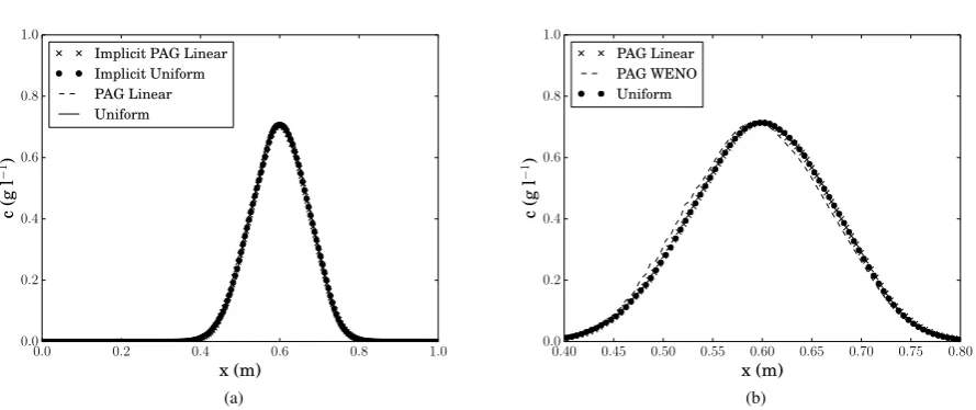
Figure 1 shows a comparison of the analytical solution with the predictions obtained using the uniform grid and
179
the PAG-linear after 0.6 min; also shown, for reference, is the result obtained using a first order scheme. As can be
observed, both of the simulated results are in excellent agreement, with the PAG-linear and uniform grid predictions
181
superimposed; however in both cases there is an error in the prediction of the peak of the analytical solution. This
182
error is seen to be similar to that shown for the schemes presented in the original reference, and is significantly greater
183
in the results using the first order scheme so is not a result of the adaptive method.
184
Figure 2 (a) and (b) and present comparisons of predictions obtained with the Implicit and IMEX temporal solvers
185
and with the PAG linear and PAG WENO reconstruction techniques and respectively. As can be seen in Figure 2 (a)
186
difference in the predictions obtained with the two temporal solver is negligible. There is, however, a slight difference
187
in the results from the two reconstructions around the peak of the profile, in order to see this clearly Figure 2 (b) shows
188
only a small interval around this region.
189
Table 3 presents the CPU runtimes for each of the simulations as well as the runtime reductions relative to the
190
benchmark of a uniform grid with the use of the Implicit solver. As can be seen, the PAG-linear results in a 86.4 %
191
CPU runtime reduction over the benchmark; while, as can be seen in Table 3, PAG-WENO enables a further 10%
192
reduction in the runtime Figure 2 (b) shows there is an additional slight error, resulting in a slight shifting of the peak
193
of the profile. Figure 2 (a) shows that use of the Implicit solver does not result in a change in the predictions, however
194
a significant increase in runtime is observed in Table 3.
195
Test 2
196
This case is again taken from Javeed et al. (2011b), and represents the injection of a single component at a rate of
197
c = 1g L−1into a column of length 1 cm, which is initially equilibriated with the solventc = 0, for 0.2 min. The 198
following non-linear isotherm is considered:
199
q(c) = c
1 +c. (29)
The values forvandǫare the same as those for Test 1 and the same number of computational cells is used, while
200
in this case the solution is computed for 3 min. In order to assess the ability of the compact WENO scheme coupled
201
with PAG method to simulate problems where both the EDM and LKM are used, this problem will be solved using
202
both of these models in turn. Where the LKM is appliedkis assumed to take the value103. The CPU runtimes for
203
simulations using both models are summarised in Table 4.
204
EDM
205
Figure 3 shows a comparison of the predicted concentration close to the end of the bed (x= 0.95) obtained using
206
uniform, PAG-linear, and PAG-WENO grids. Also shown, in the absence of an analytical solution to the problem, is a
207
reference solution which obtained using a uniform grid of 2000 computational cells. From the figure it can clearly be
208
observed that use of a relatively small mesh size results in an under-prediction of the concentration peak, nevertheless
209
the use of the PAG method does not accentuate this problem and, as shown in Table 4, results in a 20 - 30 % reduction
210
in runtime though, as seen in Test 1, the use of the PAG-WENO results in a delay in the time at which the profile
211
reaches the point at which the histories are presented. Furthermore, as with Test 1, the two temporal solvers produced
identical results.
213
LKM
214
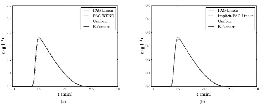
As in the case of the EDM above, Figure 4 (a) shows the comparisons of the predicted concentration histories at
215
x= 0.95using the uniform grid as well as PAG-linear and PAG-WENO reconstructions while Figure 4 (b) presents
216
the same comparison for the IMEX and implicit solvers.
217
Notably, the maximum of the peak is lower with the use of the LKM than is seen with the EDM, which is due to the
218
delay in adsorption incorporated into the model; also the predictions with smaller grids are in much better agreement
219
with the reference solution.
220
As with the above cases, 4 (a) shows that the WENO reconstruction results in a slight delay in the propagation
221
of the front; furthermore, the implicit solver also slightly increases the diffusion of the peak of the profile. As can
222
be seen in Table 4 the runtimes associated with all of the LKM simulations are significantly lower than those for the
223
EDM, which is as a result of the removal of the nested solution of the algebraic equation (5), with the PAG-linear
224
method resulting in a further 30 % decrease.
225
Test 3
226
As both Tests 1 and 2 were concerned with single components for Test 3 we select the problem presented by
227
Shipilova et al. (2008) where the LKM is applied to a two component system. In this case a competitive Langmuir
228
isotherm is used, that is for componentn:
229
qn(c) =
ancn
1 +P
jbjcj
(30) A rectangular pulse of a liquid mixture containing the two components is injected into the column for the first 1.2
230
min of the problem; after this period the concentration of the two components in the incoming stream drops to zero.
231
Table 1 presents the various parameters used, as with the previous tests, 200 computational cells were used for the
232
uniform grid and 4 min of the problem were simulated. Table 5 shows the CPU runtimes recorded in each case.
233
Figures 5 (a) and (b) show respectively a comparison of the predictions produced using a uniform grid and the
234
PAG-linear and PAG-WENO, and the comparison of the results obtained by applying the IMEX and Implicit solvers
235
respectively. As can be seen in 5 (a), as in the above cases, the predictions obtained using the PAG method are in
236
reasonable agreement with those from the uniform grid. There are two exceptions worth noting: firstly, where
PAG-237
linear is used, the end of the rectangular pulse at approximately 2 min is diffused, with the drop in concentration
238
beginning 0.4 min before that in observed in the uniform solution, the same effect using the WENO reconstruction is
239
almost negligible; secondly, that the PAG-WENO shows a slight delay in the arrival of the sharp front atca.0.7 min.
240
Likewise, Figure 5 (b) shows that implicit PAG-linear solution provides a far better resolution of the solution around
241
2 min, but diffuses the front at 0.7 min to a greater extent.
242
Figure 6 shows the same results of the PAG-linear and PAG-WENO obtained using the IMEX solver, this time
243
obtained using an initial grid of 1000 cells. As can be seen, even with the greater number of cells the PAG-linear
diffuses the wave at 2 min, while in contrast the PAG-WENO accurately resolves all parts of the solution. In this case
245
the simulation was only performed using the IMEX solver.
246
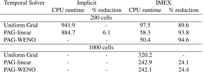
From Table 5, firstly, it can been seen that the implicit solver required runtimes at least 10 times longer than the
247
equivalent for the IMEX solver. For the finer grid simulations, where comparison is given against a uniform grid with
248
the IMEX solver only, less of a runtime reduction was observed as compared to the coarser grid.
249
Test 4
250
The previous tests have investigated problems on a small interval, for Test 4 we analyse the three component
251
displacement problem presented by Javeed et al. (2011a) which uses a much larger column length. This problem
252
consists of the injection of a rectangular pulse of the first two components (c1andc2) for 0.2 s, without the presence
253
of the third component, followed by the injection of only the third displacer component. The key parameters and feed
254
compositions are presented in Table 2. In this test, due to the larger domain, 1000 computational cells were used for
255
the uniform grid while the simulation time was 18 min.
256
Figure 7 presents profiles of the the solution obtained using a uniform grid with the IMEX solver att =1, 4, 8,
257
12 and 16 min. As can be seen the pulses, of components 1 and 2 propagate through the domain and are resolved
258
into rectangular pulses of pure components by the second half of the domain. Figures 8 (a) and (b) show comparisons
259
of the uniform grid predictions with the PAG-linear grid at the same times for the components 1 and 2 respectively,
260
as with the previous tests the error associated with the adaptive grid is negligible but results in a 66 % reduction
261
in runtime (Table 6). Also shown are the PAG-linear predictions obtained using the Implicit solver, the results are
262
similar although, as can be seen in Figure 8c as before the implicit solver results in an increased diffusion around the
263
discontinuities; as before the runtime required for the implicit is over twice that for the IMEX.
264
Conclusions
265
The simulation of chromatographic separation problems requires the solution of a system of nonlinear partial
266
differential-algebraic equations. Regardless of the model applied, a particular complexity of the equations is that,
267
under certain conditions, discontinuous profiles or shocks can form; the resolution of such profiles is challenging and
268
requires the selection of an appropriate accurate numerical scheme, while being careful to maintain computational
269
efficiency.
270
This paper presented the application of a high order numerical method which is coupled with the Piecewise
Adapt-271
ive Grid method (PAG) in order to reduce the additional computational overhead associated with its use. Importantly,
272
due to the nonuniform structure of grid used as part of the PAG method, the particular numerical scheme selected, a
273
compact WENO method, was one of the few applicable to such grids. To further increase the efficiency while
im-274
proving the accuracy of predictions, the impact of the use of explicit and Implicit-Explicit (IMEX) Runge-Kutta as
275
compared to the commonly applied fully implicit BDF method was investigated.
276
Application of the scheme to the simpler Equilibrium Dispersive Model (EDM) for single component, smooth and
277
discontinuous problems showed that an efficiency penalty, in terms of the CPU runtime, is observed relative to the
simpler first order methods; however the accuracy of solutions, for relative coarse meshes is far greater, as is expected.
279
The PAG method goes some way to mitigate the increase in decrease in efficiency even for the simplest problems, by
280
reducing the runtime by up toca. 35 %, without an observable deterioration in the solution. It was found that the
281
explicit temporal solver was up to 6 times more efficient that the implicit solver.
282
Extension to problems where the Lumped Kinetic Model was applied, and hence the use of an IMEX rather than a
283
explicit Runge-Kutta method, showed an increase in efficiency over the EDM. As the problems with a greater number
284
of components were investigated a larger reduction in the CPU runtime was observed with the application of the PAG
285
method; this is due to the greater computational weight per cell in the grid used, in a similar manner to the results
286
observed in Brown et al. (2015b).
287
Finally, the reconstruction of the solution required following the construction of the new grid, part of the PAG
288
algorithm (Brown et al., 2015b), using the underlying WENO reconstruction rather than the linear interpolation used
289
in our previous work resulted in an increase in computational efficiency. Overall, the use of PAG for industrially
290
relevant problems requiring an implicit solver resulted in upto 90% fall in runtime.
291
References
292
Ascher, U., Ruuth, S., Spiteri, R., 1997. Implicit-explicit Runge-Kutta methods for time-dependent partial differential equations. Applied Numerical 293
Mathematics 25 (2-3). 294
Berger, M., Oliger, J., 1984. Adaptive mesh refinement for hyperbolic partial differential equations. J. Comput. Phys. 53 (3), 484–512. 295
Brown, S., Fraga, E., Mahgerefteh, H., Martynov, S., 2015a. A geometrically based grid refinement technique for multiphase flows. Computers & 296
Chemical Engineering 82, 25–33. 297
Brown, S., Martynov, S., Mahgerefteh, H., 2015b. Modelling heat transfer in flashing CO2 fluid upon rapid decompression in pipelines. In:
298
Proceedings of 8th International Conference on Computational and Experimental Methods in Multiphase and Complex Flow. To appear. 299
Brown, S., Martynov, S., Mahgerefteh, H., Chen, S., Zhang, Y., 2014. Modelling the non-equilibrium two-phase flow during depressurisation of 300
CO2pipelines. Int. J. Greenhouse Gas Control 30, 9–18.
301
Butcher, J., 2008. Numerical Methods for Ordinary Differential Equations. Wiley. 302
Chan, S., Titchener-hooker, N., Bracewell, D. G., Sørensen, E., 2008. A Systematic Approach for Modeling Chromatographic Processes â ˘AˇT 303
Application to Protein Purification 54 (4), 965–977. 304
Close, E. J., Salm, J. R., Bracewell, D. G., Sorensen, E., jul 2014. Modelling of industrial biopharmaceutical multicomponent chromatography. 305
Chemical Engineering Research and Design 92 (7), 1304–1314. 306
URLhttp://www.sciencedirect.com/science/article/pii/S0263876213004425
307
Coimbra, M. d. C., Sereno, C., Rodrigues, A., 2004. Moving finite element method: applications to science and engineering problems. Computers 308
& Chemical Engineering 28 (5), 597–603. 309
URLhttp://linkinghub.elsevier.com/retrieve/pii/S0098135404000286
310
Enmark, M., Arnell, R., Forssén, P., Samuelsson, J., Kaczmarski, K., Fornstedt, T., 2011. A systematic investigation of algorithm impact in 311
preparative chromatography with experimental verifications. Journal of Chromatography A 1218 (5), 662–672. 312
URL http://dx.doi.org/10.1016/j.chroma.2010.11.029http://linkinghub.elsevier.com/retrieve/pii/
313
S0021967310016031 314
Fraga, E. S., 1998. Simulation of a fixed bed system using a geometrically based adaptive grid method. Comput. Chem. Eng. 22, 897–900. 315
Fraga, E. S., Morris, J. L., Jul. 1992. An adaptive mesh refinement method for nonlinear dispersive wave equations. J. Comput. Phys. 101 (1), 316
Fraga, E. S., Morris, J. L., 1996. A piecewise uniform adaptive grid algorithm for nonlinear dispersive wave equations. In: Griffiths, D. F., Watson, 318
G. A. (Eds.), Numerical Analysis: A R Mitchell 75thBirthday Volume. World Scientific Publishing Company, Singapore, pp. 99–124. 319
Gourma, M., Jia, N., Thompson, C., 2013. Adaptive mesh refinement for two-phase slug flows with ana prioriindicator. Int. J. Multiphase Flow 320
49, 83–98. 321
Guiochon, G., Shirazi, D., Felinger, A., Katti, A., 2006. Fundamentals of Preparative and Nonlinear Chromatography. Academic Press. 322
Hahn, T., Sommer, A., Osberghaus, A., Heuveline, V., Hubbuch, J., 2014. Adjoint-based estimation and optimization for column liquid chromato-323
graphy models. Computers & Chemical Engineering 64, 41–54. 324
Hindmarsh, A. C., Brown, P. N., Grant, K. E., Lee, S. L., Serban, R., Shumaker, D. E., Woodward, C. S., 2005. Sundials: Suite of nonlinear and 325
differential/algebraic equation solvers. ACM Transactions on Mathematical Software (TOMS) 31 (3), 363–396. 326
Javeed, S., Qamar, S., Seidel-Morgenstern, A., Warnecke, G., 2011a. A discontinuous Galerkin method to solve chromatographic models. Journal 327
of Chromatography A 1218 (40), 7137–7146. 328
Javeed, S., Qamar, S., Seidel-Morgenstern, A., Warnecke, G., 2011b. Efficient and accurate numerical simulation of nonlinear chromatographic 329
processes. Computers & Chemical Engineering 35 (11), 2294–2305. 330
Kelling, R., Bickel, J., Nieken, U., Zegeling, P., 2014. An adaptive moving grid method for solving convection dominated transport equations in 331
chemical engineering. Comput. Chem. Eng. 71, 467–477. 332
Levy, D., Puppo, G., Russo, G., 2000. Compact central weno schemes for multidimensional conservation laws. SIAM J. Sci. Comput. 22 (2), 333
656–672. 334
Mazzotti, M., 2009. Nonclassical composition fronts in nonlinear chromatography: Delta-shock. Industrial and Engineering Chemistry Research 335
48 (16), 7733–7752. 336
Medi, B., Amanullah, M., 2011. Application of a finite-volume method in the simulation of chromatographic systems: Effects of flux limiters. 337
Industrial and Engineering Chemistry Research 50 (3), 1739–1748. 338
Pais, L. S., Loureiro, J. M., Rodrigues, a. E., 1998. Modeling strategies for enantiomers separation by SMB chromatography. AIChE Journal 44 (3), 339
561–569. 340
Pelanti, M., LeVeque, R. J., Jan. 2006. High-Resolution Finite Volume Methods for Dusty Gas Jets and Plumes. SIAM J. Sci. Comput. 28 (4), 341
1335–1360. 342
Püttmann, A., Schnittert, S., Leweke, S., von Lieres, E., 2016. Utilizing algorithmic differentiation to efficiently compute chromatograms and 343
parameter sensitivities. Chemical Engineering Science 139, 152–162. 344
Russell, R. D., Christiansen, J., 1978. Adaptive mesh selection strategies for solving boundary value problems. SIAM Journal on Numerical 345
Analysis 15 (1), 59–80. 346
Semplice, M., Coco, A., Russo, G., 2015. Adaptive Mesh Refinement for Hyperbolic Systems Based on Third-Order Compact WENO Reconstruc-347
tion. Journal of Scientific Computing. 348
Sereno, C., Rodrigues, A., Villadsen, J., 1991. The moving finite element method with polynomial approximation of any degree. Computers and 349
Chemical Engineering 15 (1), 25–33. 350
Shipilova, O., Sainio, T., Haario, H., 2008. Particle transport method for simulation of multicomponent chromatography problems. Journal of 351
Chromatography A 1204 (1), 62–71. 352
Tang, H., Tang, T., 2003. Adaptive Mesh Methods for One- and Two-Dimensional Hyperbolic Conservation Laws. SIAM Journal on Numerical 353
Analysis 41 (2), 487. 354
von Lieres, E., Andersson, J., 2010. A fast and accurate solver for the general rate model of column liquid chromatography. Computers & Chemical 355
Engineering 34 (8), 1180–1191. 356
Zabusky, N., Kruskal, M., Aug 1965. Interaction of "solitons" in a collisionless plasma and the recurrence of initial states. Phys. Rev. Lett. 15, 357
240–243. 358
Zhang, Y., Feng, L., Seidel-Morgenstern, A., Benner, P., 2017. Accelerating optimization and uncertainty quantification of nonlinear SMB chro-359
Table 1: Parameters used in Test 3.
Parameters Value
Column length (cm) 1
Porosity 0.4
Velocity (cm min−1) 1
Dispersion Coefficient (cm2min−1) 10−4
Lumped mass transfer coefficient (min−1) 103
Henry coefficients a1= 0.5,a2= 1 Constants used in Eq (3) b1= 0.05,b2= 0.1 Feed concentrations (gl−1) c
[image:16.595.165.432.525.639.2]1= 10,c2= 10
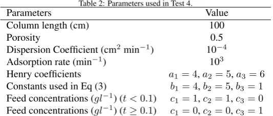
Table 2: Parameters used in Test 4.
Parameters Value
Column length (cm) 100
Porosity 0.5
Dispersion Coefficient (cm2min−1) 10−4
Adsorption rate (min−1) 103
Henry coefficients a1= 4,a2= 5,a3= 6 Constants used in Eq (3) b1= 4,b2= 5,b3= 1 Feed concentrations (gl−1) (t <0.1) c1= 1,c2= 1,c3= 0
Table 3: Summary of CPU runtimes in seconds and % reduction in runtimes relative to the Implicit uniform grid solution for Test 1.
Temporal Solver Implicit IMEX
CPU runtime % reduction CPU runtime % reduction
Uniform Grid 291.6 - 53.0 81.8
PAG-linear 256.3 12.1 39.6 86.4
PAG-WENO 276.8 5.1 34.0 88.3
Table 4: Summary of CPU runtimes in seconds and % reduction in runtimes relative to the Implicit uniform grid solution for Test 2.
Temporal Solver Implicit IMEX
CPU runtime % reduction CPU runtime % reduction EDM
Uniform Grid 941.9 - 167.7 82.2
PAG-linear 892.4 5.3 133.8 85.8
PAG-WENO 884.7 6.1 120.5 87.2
LKM
Uniform Grid 289.2 - 12.1 95.8
PAG-linear 243.6 15.8 8.4 97.1
[image:17.595.133.465.402.526.2]PAG-WENO - - 11.9 95.9
Table 5: Summary of CPU runtimes in seconds and % reduction in runtimes relative to the Implicit and IMEX uniform grid solutions for 200 and 1000 cells respectively for Test 3.
Temporal Solver Implicit IMEX
CPU runtime % reduction CPU runtime % reduction 200 cells
Uniform Grid 941.9 - 97.5 89.6
PAG-linear 884.7 6.1 58.3 93.8
PAG-WENO - - 50.4 94.6
1000 cells
Uniform Grid - - 320.2
-PAG-linear - - 242.9 24.1
PAG-WENO - - 242.1 24.4
Table 6: Summary of CPU runtimes in seconds and % reduction in runtimes relative to the Implicit uniform grid solution for Test 4
Temporal Solver Implicit IMEX
CPU runtime % reduction CPU runtime % reduction
Uniform Grid 424.5 - 165.4 61.0
0.0 0.2 0.4 0.6 0.8 1.0
x (m)
0.0 0.2 0.4 0.6 0.8 1.0
c
(g
l
−
1)
[image:18.595.186.398.110.286.2]PAG Analytical First order Uniform Uniform
Figure 1: Comparison of the analytical solution with the numerical solutions forcfor Test 1 computed using a uniform grid of 200 cells and an equivalent piecewise adaptive grid with a linear reconstruction (PAG-linear) att=0.6 min.
0.0 0.2 0.4 0.6 0.8 1.0
x (m)
0.0 0.2 0.4 0.6 0.8 1.0
c
(g
l
−
1)
Implicit PAG Linear Implicit Uniform PAG Linear Uniform
(a)
0.40 0.45 0.50 0.55 0.60 0.65 0.70 0.75 0.80
x (m)
0.0 0.2 0.4 0.6 0.8 1.0
c
(g
l
−
1)
PAG Linear PAG WENO Uniform
(b)
[image:18.595.77.522.352.539.2]1.0 1.5 2.0 2.5 3.0
t (min)
0.0 0.1 0.2 0.3 0.4 0.5
0.6
c
(g
l
−
1)
[image:19.595.187.396.164.329.2]PAG Linear PAG WENO Uniform Reference
Figure 3: Predicted variation ofcwith time atx= 0.95cm computed using the Equilibrium Dispersive Model (EDM) for Test 2 with a uniform
grid, as well as PAG-linear and PAG-WENO reconstructions also shown is a reference solution obtained using 2000 uniform cells.
1.0 1.5 2.0 2.5 3.0
t (min)
0.0 0.1 0.2 0.3 0.4 0.5 0.6
c
(g
l
−
1)
PAG Linear PAG WENO Uniform Reference
(a)
1.0 1.5 2.0 2.5 3.0
t (min)
0.0 0.1 0.2 0.3 0.4 0.5 0.6
c
(g
l
−
1)
PAG Linear Implicit PAG Linear Uniform
Reference
(b)
Figure 4: Predicted variation ofcwith time atx= 0.95cm computed using the LKM withk= 103
[image:19.595.75.524.471.652.2]0.0 0.5 1.0 1.5 2.0 2.5 3.0 3.5 4.0
t (min)
0 5 10 15 20
c
(g
l
−
1)
c1, PAG Linear
c2, PAG Linear
c1, PAG WENO
c2, PAG WENO
c1, Uniform
c2, Uniform
(a)
0.0 0.5 1.0 1.5 2.0 2.5 3.0 3.5 4.0
t (min)
0 5 10 15 20
c
(g
l
−
1)
c1, PAG Linear
c2, PAG Linear
c1, Implicit PAG Linear
c2, Implicit PAG Linear
[image:20.595.81.521.172.351.2](b)
Figure 5: Predicted variation ofc1andc2with time atx= 0.5cm for Test 3 with (a) a uniform grid, as well as PAG-linear and PAG-WENO
reconstructions (b) IMEX and implicit solvers respectively; also shown is a reference solution obtained using 2000 uniform cells.
0.0 0.5 1.0 1.5 2.0 2.5 3.0 3.5 4.0
t (min)
0 5 10 15 20
c
(g
l
−
1)
c1, PAG Linear
c2, PAG Linear
c1, PAG WENO
c2, PAG WENO
c1, Uniform
c2, Uniform
(a)
Figure 6: Predicted variation ofc1andc2with time for Test 3 atx = 0.5cm using a uniform grid, as well as PAG-linear and PAG-WENO
[image:20.595.187.397.472.660.2]0
20
40
60
80
100
0
.
0
0
.
2
0
.
4
0
.
6
0
.
8
[image:21.595.132.462.279.530.2]1
.
0
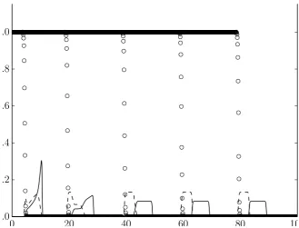
Figure 7: Variation ofc1,c2andc3 along the length of the bed at 1, 4, 8, 12 and 16 min for Test 4 predicted using a uniform grid of 1000
x (cm) 0
20 40
60 80
100
t (m in)
0 2
4 6 8
10 1214
16
c
(g
l
−
1)
0.00 0.05 0.10 0.15 0.20 0.25 0.30 0.35 0.40
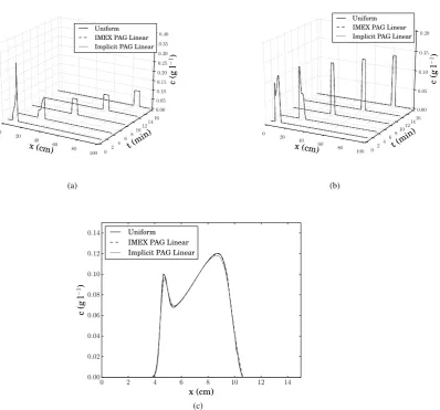
Uniform IMEX PAG Linear Implicit PAG Linear
(a)
x (cm) 0
20 40
60 80
100 t (
min )
0 2
46 810
1214 16
c
(g
l
−1
)
0.00 0.05 0.10 0.15 0.20
Uniform IMEX PAG Linear Implicit PAG Linear
(b)
0 2 4 6 8 10 12 14
x (cm)
0.00
0.02
0.04
0.06
0.08
0.10
0.12
0.14
c
(g
l
−
1)
Uniform IMEX PAG Linear Implicit PAG Linear
[image:22.595.118.517.234.605.2](c)
Figure 8: Variation ofc1(a) andc2(b) along the length of the bed at 1, 4, 8, 12 and 16 min predicted using the IMEX and implicit temporal solvers