Infrared Camera Imaging Algorithm to Augment
CT-Assisted Biopsy Procedures
John Leis
Electrical, Electronic andComputer Engineering University of Southern Queensland
Toowoomba, Queensland 4350 Email: [email protected]
Behrooz Sharifi
Radiology DepartmentPACS RIS Unit Princess Alexandra Hospital
Brisbane, Queensland
Email: behrooz [email protected]
Abstract—The problem with CT guided biopsies is the high dosage of radiation exposure to the patient, the time it takes to perform the procedure and the lack of spatial reference of the operator. We approach this problem by using a system comprising of two digital infrared sensitive cameras and a high intensity infrared illuminator which was used to capture the coordinates of an infrared reflective tape attached to a coaxial biopsy needle having been inserted into a test phantom. Data was sent in real-time to a computer where the infrared needle position coordinates were recorded. A CT scan of the test phantom was then taken and the DICOM CT image coordinates of the needle were also recorded. The approach is to use a linear least-squares model to map points from each camera to a single point on each DICOM CT image resulting from the CT scan. Results show a promising mapping accuracy with limited data. The contribution of this paper is to show that a passive infrared imaging system using at least two cameras may be suitable for the needle estimation task in two dimensions which would allow real-time needle placement in any plane.
I. INTRODUCTION
Computed tomography (CT) is a process widely used in the medical field for imaging anatomic information from a cross-sectional plane of the body [1]. One useful application of CT is in guided surgical routines, where CT images assist in guiding the tools and equipment necessary to perform procedures at the appropriate areas of the body. CT guided procedures include biopsies where a sample of tissue needs to be extracted from patients body using a biopsy needle for further analysis and fine needle aspirations where a thin needle is passed through the skin to sample fluid or tissue from a cyst or solid mass of the lung, liver, nodes, bones, etc. There are also therapeutic injections of joints, nerve roots and epidural, also radiofrequency ablation and drain placements [2].
Steps currently involved in performing a freehand CT guided biopsy procedure include [3]:
1) Positioning the patient, applying skin markers and per-forming a CT scan;
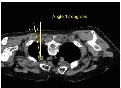
2) Assessing the image for safe biopsy path, measuring the desired entry angle and determining the skin entry point (Fig. 1);
3) Marking the skin entry point on the patient; 4) Inserting the biopsy needle at predicted angle;
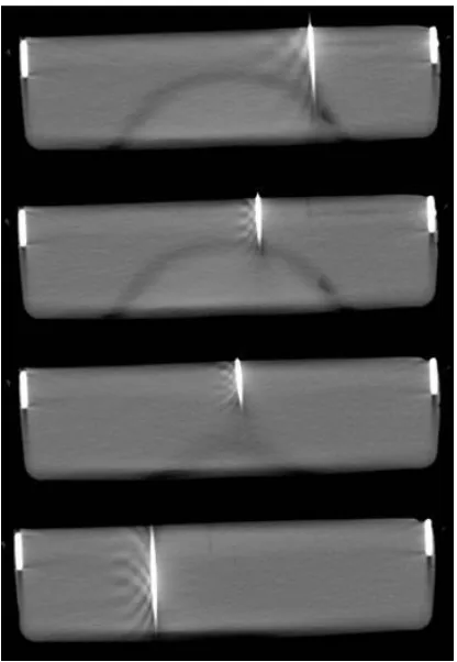
5) Advancing the needle in a stepwise fashion, re-imaging the patient at each step to determine any required corrections in trajectory (Fig. 2); and
6) Confirming the needle position prior to taking biopsy.
[image:1.612.322.552.381.548.2]Inserting the biopsy needle at a predicted angle and advanc-ing it along a desired path is a challengadvanc-ing task that requires much practice and experience as well as sound judgement in spatial reference. To ensure the accuracy and safety of the procedure, the radiologists typically advance the needle in a stepwise fashion, re-imaging the patient at each stage to determine any required corrections in trajectory.
Fig. 1. Biopsy path with the desired entry angle.
Fig. 2. Advancing the needle in a stepwise fashion.
which reduces or eliminate radiation dose must be made available for radiographic procedures. ALARA is not only a sound safety principle, it is a regulatory requirement for all radiation proceedures [4].
There are also some biopsy scenarios where the lesion being biopsied is difficult to get to. In such scenarios, the radiologists use double angle, i.e., the needle is angled in two planes, left/right and up/down. In order to hit the target, the angles need to be very precise. At present to get around this, the CT gantry is tilted to the required angle. The radiologist then inserts the needle into the patient, and uses the gantry laser lights as a guide for the up/down angle as required [5]. Laser guidance devices are also used to help guide probe placement in order to reduce procedure time and improve targeting accuracy [6]. Newer CT scanners, however, are often unable to tilt the gantry because of size and engineering challenges [7]. Consequently, there is a developing need for an alternative method of performing the double angled biopsies under CT-guidance.
An infrared guided biopsy needle system may assist the operator and could be used as an alternative method. In order to work towards this, we describe a method to estimate computed tomography image points from multiple infrared measurements. A system comprising a digital infrared sen-sitive camera and high intensity infrared illuminator was used to capture the position of an infrared reflective tape attached to a coaxial biopsy needle (Fig. 3) having been inserted into a marked insertion point on a test phantom. Data was sent in real-time to a computer where using custom software, needle entry position was displayed and coordinates captured (Fig. 4). Then without moving the test phantom a CT scan was taken of the phantom with the needle still fixed in the entry position. The entry point coordinates of the DICOM (Digital Imaging and Communications in Medicine) image were also recorded (Fig. 5).
Fig. 3. The needle with an infrared reflective tape attached. Infrared emitters and Wii cameras fixed and a phantom with 20 entry marks.
Fig. 4. IR Results - Entry point values (u, v) of each infrared camera capture (camera 1 and 2).
II. NEEDLEPOSITIONESTIMATION
Figure 6 illustrates the mapping problem which we address. To simplify the problem, we focus on a single target point
(x, y)on the DICOM image. This point makes an image point
(u1, v1)on camera 1, and(u2, v2)on camera 2.
[image:2.612.59.292.52.224.2] [image:2.612.337.537.359.567.2]ex-Fig. 5. DICOM images from CT scans. the needle is inserted on the marked entry points and a CT scan taken.
DICOM(x, y)plane
IR
(u 1, v
1)
plane
IR
(u2, v2 )plane
b
b
[image:3.612.71.279.52.353.2]b
Fig. 6. Imaging of the needle position in the DICOM image on the two IR cameras. The inverse problem – mapping from IR camera measurements to DICOM position – is the prime focus of this paper.
posure for the patient, yet it is necessary in order estimate the needle position with reasonable accuracy. A passive infrared system, as described, could estimate the needle position by extrapolation of previous calibration points.
III. LINEARESTIMATION OFNEEDLE ONDICOM IMAGE
FROMIR CAMERASALONE
We perform N sets of IR-CT calibration tests, each com-prisingM IR cameras (M = 2in the present work). Denote
the output DICOM image position by(xn, yn)wherenis the
measurement set index. Thus the vector of targets (desired CT positions) is
x =
x1 y1
x2 y2 .. . ...
xN yN
(1)
The IR camera measurements are (un,m, vn,m) for camera
m and target point n. In the present work with 2 cameras,
M = 2and each measurement point comprises a vectormn=
[un,1, vn,1, un,2, vn,2]T.
We assume that each measurement is linearly proportional to the camera spot measurements, and that these are independent. Denoting each IR output as(un,m, vn,m)for sensor mwithin
measurement setn, the linear model is constructed as follows. For thex-component, we have
x1 = a0+a1u1,1+a2v1,1+a3u1,2+a4v1,2+· · ·+
a2M−1u1,M+a2Mv1,M
x2 = a0+a1u2,1+a2v2,1+a3u2,2+a4v2,2+· · ·+
a2M−1u2,M+a2Mv2,M
.. .
xN = a0+a1uN,1+a2vN,1+a3uN,2+a4vN,2+· · ·+
a2M−1uN,M+a2MvN,M
overN calibration measurements.
Similarly, for they-component, we have
y1 = b0+b1u1,1+b2v1,1+b3u1,2+a4v1,2+· · ·+
b2M−1u1,M+b2Mv1,M
y2 = b0+b1u2,1+b2v2,1+a3u2,2+a4v2,2+· · ·+
b2M−1u2,M+b2Mv2,M
.. .
yN = b0+b1uN,1+b2vN,1+b3uN,2+b4vN,2+· · ·+
b2M−1uN,M+b2MvN,M
The equation defining mapping IR→CT for 2 cameras is is then formed (for the specific case ofM = 2 cameras) as
x1 y1
x2 y2 .. . ...
xN yN
=
1 u1,1 v1,1 u1,2 v1,2
1 u2,1 v2,1 u2,2 v2,2 ..
. ...
1 uN,1 vN,1 uN,2 vN,2
a0 b0
a1 b1
a2 b2
a3 b3
a4 b4
(2)
This may be written as
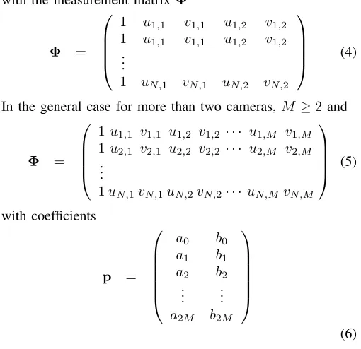
[image:3.612.60.292.393.558.2]with the measurement matrix Φ Φ =
1 u1,1 v1,1 u1,2 v1,2
1 u1,1 v1,1 u1,2 v1,2 ..
.
1 uN,1 vN,1 uN,2 vN,2
(4)
In the general case for more than two cameras, M ≥2 and
Φ =
1u1,1 v1,1 u1,2 v1,2 · · · u1,M v1,M
1u2,1 v2,1 u2,2 v2,2 · · · u2,M v2,M
.. .
1uN,1vN,1uN,2vN,2· · · uN,MvN,M
(5) with coefficients p =
a0 b0
a1 b1
a2 b2 .. . ...
a2M b2M
(6)
The above represents an over-determined system, and in practice will have only an approximate solution due to mea-surement noise. Thus we require the minimum of
||x−Φp|| (7)
This may be estimated in several ways, and here we use a min-imum least-squares solution. Denoting the optimal prediction coefficients by
p∗ =
a0 b0
a1 b1
a2 b2 .. . ...
a2M b2M
(8)
the optimal solution which minimizes the least-squares dis-tance betweenxandΦpis the Moore-Penrose pseudoinverse
p∗ = ΦTΦ−1
ΦTx (9)
We now have the error vector
εεε = x−xb (10)
= x−Φ p (11)
where the error vector is
εεε =
εx1 εy1
εx1 εy1
.. . ...
εxN εyN
(12)
If the IR image points are correlated, the inverse in (9) may not exist. This is one practical limitation of the problem, and requires careful consideration when implemented. In particu-lar, if one camera is occluded, a solution becomes impossible. Furthermore, it is conceivable that excessive skew of one of the
cameras may result in numerical instabilities, thus producing unreliable estimates.
The calibration of the system is performed by measuring
(x, y) points on the DICOM image, and utilizing the corre-sponding (u, v) IR camera points. Presently, the IR camera points are automatically determined, though this may require further investigation in the case of imperfect infrared lighting conditions. The DICOM image points are determined manu-ally; this is a somewhat time-consuming task, and one goal not addressed here is to automate this aspect of the procedure. Once the calibration procedure and pseudoinverse is calcu-lated, the parameters p∗ are known (or at least estimated), and the DICOM image points may be estimated using a straightforward multiplication of vectors for each point
b
xn = [1|φφφn] p∗ (13)
whereφφφn is the vector of(u, v)point pairs obtained for each
measurement, resulting in the predicted DICOM image points
(xn, yn)inxbn. This then allows overlaying of the estimated
position on the most recently acquired DICOM image.
[image:4.612.48.303.63.310.2]IV. RESULTS
Table I shows the measured IR image points on each camera with the corresponding DICOM measurements. Note that all co-ordinates are scaled in pixel co-ordinates, thus it is unnecessary to attempt to translate back to real-world measurements using this approach. The goal is that the image is merely presented as a DICOM image to the surgery staff with the IR points overlaid.
TABLE I
EXPERIMENTAL DATA FOR INFRARED CAMERA PAIR TOCTIMAGE POINTS.
Infrared DICOM
coordinates coordinates
u1 v1 u2 v2 x y
247 243 473 244 1084 528
209 244 439 251 943 533
220 133 461 144 966 526
245 244 479 251 1109 529
224 133 486 140 903 525
199 126 411 134 785 527
113 125 364 139 632 531
89 134 323 140 447 535
50 126 346 145 355 544
160 130 407 141 651 539
98 234 358 239 441 536
21 126 281 133 267 540
43 244 270 252 275 555
188 120 412 125 873 525
91 120 364 126 682 530
82 117 345 123 523 528
24 117 293 133 325 534
This of course is not realistic, but does however serve to go some way to suggesting the usefulness of the technique and soundness of the underlying assumptions.
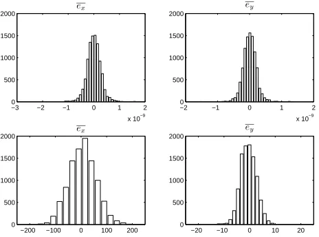
The lower two plots of Figure 7 show the error distributions when selecting unseen data. The entire data set is partitioned into “train” and “test” data subsets, where the “train” subset is used to estimate the predictor coefficients and the “test” subset is used to validate the predictions using the estimated coefficients. In the present case, approximately 75% of the data was used for training, and the remainder for testing. The selection of test/train data was done randomly, and the selection repeated in a Monte-Carlo iteration.
The prediction of the parameters appears to be quite good, and generally somewhat better than the histogram would sug-gest. We attribute this to singular errors in the measurements, which may skew the predictions.
Errors in DICOM Estimation for Seen and Unseen IR Measurements
−3 −2 −1 0 1 2
x 10−9 0
500 1000 1500
2000 ex
−2 −1 0 1 2
x 10−9 0
500 1000 1500 2000
ey
−200 −100 0 100 200 0
500 1000 1500 2000
ex
−20 −10 0 10 20
0 500 1000 1500 2000
[image:5.612.59.291.288.460.2]ey
Fig. 7. Histograms of errors in random trials: prediction using known data (top), and prediction using unseen data (lower).
V. BOOTSTRAPPARAMETERRE-ESTIMATION
Because the accuracy of the resulting device is a paramount concern, and the fact that the calibration data is difficult and time-consuming to acquire, we analyse the parameters using a bootstrap approach. The bootstrap method has been utilized in the signal processing community [8], [9], [10] and has been employed where data is very difficult or time-consuming to acquire (for example, [11], [12]). The experimental data was very time-consuming to acquire and because of the expensive nature of the CT equipment, the continuous usage of such equipment, and the need to carefully follow radiation safety procedures, using the bootstrap approach was deemed to be a reasonable approach to estimating the efficacy of the method. Empirical distributions for the predictor parameters can be established using the bootstrap estimate, as follows [9]. The predictor pˆ is estimated using the pseudoinverse as before.
Then the estimated output and error are calculated as
ˆ
x = Φpˆ (14)
ˆ
εεε = x−ˆx (15)
We then resampleεεεˆto give
b
x∗ = Φpb+bεεε
∗
(16)
b
p∗(b) = ΦTΦ−1
ΦTxb∗ (17)
The resulting bootstrap estimates are shown in Figure 8 for theM = 2cameras. It is interesting to note that coefficientsa1 througha4andb1 throughb4indicate a convergence, whereas coefficientsa0andb0indicate a large magnitude with roughly uniform spread. We attribute this to the relative scaling of the IR image planes as compared to the DICOM image, since the first coefficient is the constant term in the predictor matrixΦ. The IR cameras have resolution of only 320×200, whereas the DICOM images are of much higher resolution, and the magnitude and distribution of this coefficient appear to reflect this fact.
−2000 −1000 0 1000 2000
a0 x¯=−138.91
450 500 550 600 650
b0 ¯x= 546.43
−2 0 2 4 6
a1 x¯= 2.15
−0.2 −0.1 0 0.1 0.2
b1 x¯= 0.00
−20 −10 0 10 20 30
a2 x¯= 3.56
−1.5 −1 −0.5 0 0.5
b2 ¯x=−0.54
−4 −2 0 2 4 6
a3 x¯= 1.45
−0.3 −0.2 −0.1 0 0.1 0.2
b3 ¯x=−0.08
−30 −20 −10 0 10 20
a4 ¯x=−3.66
Bootstrap Re-estimation of Mapping Parameters
−0.5 0 0.5 1 1.5
[image:5.612.319.551.314.497.2]b4 x¯= 0.62
Fig. 8. Bootstrap results showing each parameter estimates using the experimental data.
VI. CONCLUSION
We have described an approach for estimating the position of a biopsy needle using passive infrared cameras, calibrated using a set of known CT scans. The mapping problem was shown to be able to be solved using a linear estimator, and the inverse (prediction) problem produced stable numerical results. Thus we have confidence in the ability of the system to provide an approximation of the biopsy needle position in two dimensions for subsequent needle manipulation, until a further CT scan is performed.
other aspects such as radial lens distortion is incorporated. Furthermore, the approach could be extended to multiple cameras so as to solve the issue of possible occlusion of one of the cameras which, with only two cameras, would render the system ineffective. Finally, a 3-dimensional approach is also under study, which would provide a 3-dimensional view of the biopsy needle position.
REFERENCES
[1] G. T. Herman, Fundamentals of Computerized Tomography: Image Reconstruction from Projections, 2nd ed. Springer Publishing Company, Incorporated, 2009.
[2] E. Seeram,Computed Tomography: Physical Principles, Clinical Appli-cations, and Quality Control, ser. Contemporary Imaging Techniques. Saunders/Elsevier, 2009.
[3] S. Dimmick, M. Jones, J. Challen, J. Iedema, U. W. U., and J. Coucher, “CT-Guided Procedures: Evaluation of a Phantom System to Teach Accurate Needle Placement,”Clinical Radiology, vol. 62, pp. 166–171, Feb 2007.
[4] T. WM., G. J., B. JJ., O. WR., and van Persijn van Meerten EL., “Patient and Staff Dose during CT Guided Biopsy, Drainage and Coagulation,”
British Journal of Radiology, vol. 74, pp. 720–726, Aug 2001. [5] W. E. Brant and N. M. Major, Fundamentals of Body CT, 3rd ed.
Philadelphia: Saunders Elsevier, 2006.
[6] Z. Varro, J. K. Locklin, and B. J. Wood, “Laser Navigation for Ra-diofrequency Ablation,”CardioVascular and Interventional Radiology, vol. 27, no. 5, pp. 512–515, 2004.
[7] P. Frederick, T. Brown, M. H. Miller, A. L. Bahr, and K. H. Taylor, “A Light-Guidance System to be used for CT-Guided Biopsy,”Radiology, vol. 154, pp. 535–536, 1985.
[8] A. M. Zoubir and D. R. Iskander, “Bootstrap Methods in Signal Processing,”IEEE Signal Processing Magazine, vol. 24, no. 4, pp. 7–8, Jul. 2007.
[9] ——, “Bootstrap Methods and Applications,”IEEE Signal Processing Magazine, vol. 24, no. 4, pp. 10–19, Jul. 2007.
[10] A. M. Zoubir, “The Bootstrap: A Tool for Signal Processing,” in Thirty-First Asilomar Conference on Signals, Systems & Computers, vol. 1, no. 4, Nov. 1997, pp. 433–437.
[11] D. C. Reid, A. M. Zoubir, and B. Boashash, “The Bootstrap Applied to Passive Aircraft Parameter Estimation,” inInternational Conference on Acoustics, Speech and Signal Processing, vol. 6, 1996, pp. 3153–3156. [12] H. Anton and R. C. Busby,Contemporary Linear Algebra. John Wiley