Tissue conductivity based human head model study for EEG

(1)

i

University of Southern Queensland, Australia

Tissue Conductivity based Human Head Model Study for

EEG

A Dissertation Submitted by

Md. Rezaul Bashar

(2)

ii

Abstract

The electroencephalogram (EEG) is a measurement of neuronal activity inside the brain over a period of time by placing electrodes on the scalp surface and is used extensively in clinical practices and brain researches, such as sleep disorders, epileptic seizure, electroconvulsive therapy, transcranial direct current stimulation and transcranial magnetic stimulation for the treatment of the long term memory loss or memory disorders.

The computation of EEG for a given dipolar current source in the brain using a volume conductor model of the head is known as EEG forward problem, which is repeatedly used in EEG source localization. The accuracy of the EEG forward problem depends on head geometry and electrical tissue property, such as conductivity. The accurate head geometry could be obtained from the magnetic resonance imaging; however it is not possible to obtain in vivo tissue conductivity. Moreover, different parts of the head have different conductivities even with the same tissue. Not only various head tissues show different conductivities or tissue inhomogeneity, some of them are also anisotropic, such as the skull and white matter (WM) in the brain. The anisotropy ratio is variable due to the fibre structure of the WM and the various thickness of skull hard and soft bones. To our knowledge, previous work has not extensively investigated the impact of various tissue conductivities with the same tissue and various anisotropy ratios on head modelling.

(3)

iii

spherically and realistically shaped head geometries for the head model construction. We also investigate the sensitivity of inhomogeneous and anisotropic conductivity on EEG computation.

(4)

(5)

v

Acknowledgements

I would like to express my gratitude to my principal supervisor A/Prof Yan Li for offering me the opportunity to perform this research under her supervision, support, motivation, encouragement, advice, comments and discussions. I owe much gratitude to my associate supervisor Dr Peng (Paul) Wen for his guidance, continuous support, encouragement, his knowledge and willingness to answer my questions, discussions about current research issues and critically evaluating my work during my whole research period. I would not imagine carrying out this research without his constant support and help.

I would like to thank Dr Guang Bin Liu, Department of Psychology for his support to understanding the most complex organ of the human body, the brain and its function at the beginning of this research. I would also like to thank A/Prof Shahjahan Khan, Department of Mathematics & Computing and Md. Masud Hasan (Sunshine Coast University) for their assistance in the understanding of statistical analysis.

I would like to thank Professor Mark Sutherland, Director of Centre for Systems Biology for the support of my partial international tuition fees and grants to attend conference.

I wish to thank my colleagues in our research group for their discussions and comments during our discussions, especially in the monthly seminars.

I also want to thank the Australian Research Council discovery grant for my scholarship, Department of Mathematics & Computing for my studentship and travel grant to attend international conferences and the higher degrees research office for International research excellence award during my study.

I would like to thank Dr Ian Weber, Learning and Teaching Support Unit, USQ and Lynne A. Higson, West Queensland for their efforts to correct my English.

Last but not least, I offer my gratitude to my wife Mst Asmaul Husna and my lovely son Md Samiul Bashar for their endless support and enduring love.

(6)

vi

List of Figures

No. Title Page

Figure 2.1 Mid sagittal view of the human brain 9

Figure 2.2 The four lobes of the brain 10

Figure 2.3 Internal structure of the brain as seen in coronal section 11 Figure 2.4 Structure of a neuron and information transmission 12

Figure 2.5 Different parts of the skull. 14

Figure 2.6 A cross sectional view of the scalp, skull and brain 15

Figure 2.7 Head muscles 15

Figure 2.8 The 10-20 international electrode system for the placement

of electrodes at the head surface 16

Figure 2.9 EEG on referential montage using Advance Source

Analysis 17

Figure 3.1 A five-layered spherical head model. 21

Figure 3.2 Head tissue classification from a raw MRI 22 Figure 3.3 Sample FEM tetrahedral mesh with tissue classification 23 Figure 3.4 Anisotropic conductivities of white matter.longrepresents

longitudinal andtransrepresents transversal conductivity

30

Figure 3.5 The linear relationship between the eigen values of the diffusion and conductivity ellipsoid. The resulting ellipsoid is identical to the diffusion ellipsoid up to an unknown scaling factor, which can be derived using the volume constraint with the isotropic conductivity sphere of white matter.

32

Figure 3.6 The linear relationship between the eigen values of diffusion tensor and conductivity values for the Wang’s constraint

33

Figure 3.7 The anisotropic skull conductivity. 34

Figure 3.8 Different conductivity values of the skull for different

(12)

xii

Figure 3.9 Fractional anisotropy for WM 38

Figure 3.10 Conductivity ratio Vs fractional anisotropy (FA). 38 Figure 3.11 Volume constrained conductivities produced by Monte

Carlo method. Conductivity analysis using histogram: (a) radial conductivities and (b) tangential conductivities

40

Figure 4.1 Boundary between two compartments. 1 and 2 are

conductivities of tissue layer 1 and 2, respectively, and the normal vector en is the interface.

45

Figure 4.2 A dipole model. r0 is the location of dipole centre. +I0 is

current source and –I0 is the current sink points. d is

distance from source to sink and I(r) is current field at a point r.

47

Figure 4.3 The angle between vectors pointing to surface position r and dipole location rq is denoted . The angle the dipole q

makes with the radial direction at rq is denoted . The angle

between the plane formed by rq and q, and the plane formed

by rq and r is denoted 

50

Figure 5.1 Spherical head model construction 59

Figure 5.2 (a) Value of conductivity ratio (lt) between longitudinal

and transverse conductivity for each WM element generated by CRA, (b) clear view of (a) from 102 to 103 WM elements, (c) longitudinal (long.) and transverse (trans.) conductivity values for each WM elements based on

lt of (a) using Volume constraint, and (d) clear view of (c)

from 102 to 103 WM elements

66

Figure 5.3 (a) Value of lt (conductivity ratio) between longitudinal

and transverse conductivity for each WM element generated by SCA, (b) clear view of (a) from 102 to 103 WM elements, (c) longitudinal and transverse conductivity values for each WM elements based on lt of (a) using

(13)

xiii

Volume constraint, and (d) clear view of (c) from 102 to 103 WM elements

Figure 5.4 Probability density function of Rayleigh distribution. 77 Figure 5.5 Inhomogeneous anisotropic conductivities produced by

SCA. (a)–(d) WM elements and (e)-(h) skull elements. 78 Figure 5.6 Effects of inhomogeneous anisotropic WM conductivity on

EEG: (a) relative errors () values (in percentage) and (b) correlation coefficient () values.

83

Figure 5.7 Effects of inhomogeneous anisotropic skull conductivity on EEG: (a) relative errors () values (in percentage) and (b) correlation coefficient () values.

84

Figure 5.8 Effects of inhomogeneous anisotropic WM and skull conductivities together on EEG: (a) relative errors () values (in percentage) and (b) correlation coefficient () values.

85

Figure 5.9 Effects of inhomogeneous anisotropic head model on EEG: (a) relative errors () values (in percentage) and (b)

correlation coefficient () values.

86

Figure 5.10 Topographic visualization of the scalp electrode potentials. (a) head model (A) and head model (D): (b) from the parallel Volume constraint, (c) from the parallel Wang’s constraint, (d) from the perpendicular Volume constraint and (e) from the perpendicular Wang’s constraint

conductivity for the first dipole (elevation angles /5.22 and azimuth angle /4).

87

Figure 6.1 Simplified local tissue conductivity based three-layered

spherical head model showing different tissues. 92 Figure 6.2 Local scalp tissue conductivity approximation. The

conductivity for scalp (skin) is 0.33 S/m, wet skin (place of electrodes) is 0.1 S/m and fat is 0.04 S/m.

93

(14)

xiv

Figure 6.4 RDM and MAG from assigning local conductivity to different layers in a three-layered spherical head model using the somatosensory cortex (SC) and the thalamic dipoles. In the above figures, label Br, Sk and Sc represent brain, skull and scalp, respectively.

97

Figure 6.5 RDM and MAG from assigning local conductivity to different layers in a four-layered spherical head model using the somatosensory cortex and the thalamic dipoles. In the above figures, label Br, Sk and Sc represent the brain, skull and scalp, respectively.

98

Figure 6.6 RDM and MAG from assigning the local conductivity to

different layers in the realistic head model for both dipoles. 100 Figure 6.7 The brain is viewed from the outer side and front with the

hippocampus and amygdala. 107

Figure 6.8 Location of one of the AD sources in RA by the cross hairs

in different views. 108

Figure 6.9 RDM (a) and MAG (b) errors from different brain tissue

distortion levels on source to source basis. 109 Figure 6.10 RDM (a) and MAG (b) errors from RA and LA sourced

without and with different brain tissue distortion levels to SC sourced normal EEG.

109

Figure 6.11 Contour view of scalp potentials obtained from somatosensory cortex (a) reference model, (b) five percent, (c) ten percent, (d) fifteen percent and (e) twenty percent brain tissue distortions.

110

Figure 6.12 Electrode positions (left ear-Nasion – right ear). Odd

number with electrode names indicate left hemisphere, even number with electrode names indicate right hemisphere.

111

Figure 7.1 WM conductivity uncertainty: (a) mean relative errors (m) and (b) mean correlation coefficient (m) values generated by incorporating WM conductivity uncertainty. RefA and

(15)

xv

RefB represent the Reference Models A and B, respectively.

long represents the longitudinal and trans represents the transversal conductivities with V for Volume constraint and

W for Wang’s constraint.

Figure 7.2 Skull conductivity uncertainty: (a) mean relative errors (m) and (b) mean correlation coefficient (m) values generated by incorporating skull conductivity uncertainty. RefA or

RefB stands for either reference model A or B. tan

represents the tangential and rad represents the radial conductivities with V for Volume constraint and W for Wang’s constraint.

119

Figure 7.3 The scalp conductivity uncertainty: (a) mean relative errors (m) and (b) mean correlation coefficient (m) values. RefA

or RefB stands for either reference model A or B. tan

represents the tangential and rad represents the radial conductivities with V for Volume constraint and W for Wang’s constraint.

(16)

xvi

List of Tables

No. Title Page

Table 3.1 Skull resistivity (reciprocal of conductivity. 24

Table 3.2 Body tissue conductivity. 25

Table 3.3 Head tissue conductivity. 26

Table 3.4 Head tissue conductivitiesused in this dissertation. 27 Table 3.5 Homogeneous and isotropic conductivities used in this

dissertation. 27

Table 4.1 Comparison among different methods for solving the

forward problem. 54

Table 5.1 Average related error () and correlation coefficient ()

values resulted by Models A and B. 63

Table 5.2 Average  and  values resulted by comparing Models A and

C. 63

Table 5.3 Average  and  values resulted by comparing Models A and

D. ₆₄

Table 5.4 RDM and MAG values between reference and computed

models for WM. 67

models for skull. 68

models for WM and skull together. 68

Table 5.7 RDM and MAG values using SCA for the WM. 70 Table 5.8 RDM and MAG values using SCA for the skull. 70 Table 5.9 RDM and MAG values using SCA for the WM and skull

together. 70

Table 5.10 RDM and MAG values generated by inhomogeneous

(17)

xvii

anisotropic skull conductivities. 73

anisotropic WM and skull conductivities. 73 Table 5.13 Average RDM and MAG errors for the WM inhomogeneous

and anisotropic conductivities for the orthogonal dipole

orientations of X, Y and Z. 74

Table 5.14 Average RDM and MAG errors for the skull inhomogeneous and anisotropic conductivities for the orthogonal dipole orientations of X, Y and Z.

75

Table 5.15 Average RDM and MAG errors for the WM and skull inhomogeneous and anisotropic conductivities for the orthogonal dipole orientations of X, Y and Z.

75

Table 5.16 RDM and MAG values produced by longitudinal

conductivities. 79

Table 5.17 RDM and MAG values produced by transverse

conductivities. 80

Table 5.18 Effects of inhomogeneous scalp tissue conductivity on EEG. 85

Table 6.1 Effects of principal tissue variations assigning local

conductivity in three-layered spherical head model. 97 Table 6.2 Effects of element variations assigning local conductivity in

four-layered spherical head model. 99

Table 6.3 Effects of element variations assigning local conductivity in

realistic head model. 101

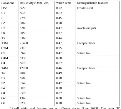
Table 6.4 Skull conductivity, width and features at different places. 102

Table 7.1 The uncertain parameter (conductivity) and its ranges used in

this study for the head model construction. 115 Table 7.2 Homogeneous conductivity values for different tissue layers

(18)

xviii

conductivity perturbations for different dipole eccentricities. Table 7.4 Sensitivity indexes for different conductivities in the

spherical head model comparing with the reference model A. 120 Table 7.5 Sensitivity indexes for different conductivities in realistic

(19)

xix

List of Acronyms

AD- Alzheimer’s disease AP – Action potential

ASA- Advanced source analysis

BEM – Boundary Element Method BEV –Brain element variation BTDL- Brain tissue distortion level

CC – Correlation coefficient CDL – Cortical dipole layer

CRA- Conductivity ratio approximation CSF – Cerebrospinal Fluid

CT- Computed tomography

DB- Dipole bunch DT- Diffusion tensor

DT-MRI- Diffusion tensor magnetic resonance imaging

EEG- Electroencephalography

FA- Fractional anisotropy FE – Finite Element

FDM – Finite Difference Method FEM – Finite Element Method

GM- Gray matter

LTC-Local tissue conductivity

MAG – Magnification factor MEG- Magnetoencephalography MLE- Maximum likelihood estimator MRI-Magnetic resonance imaging

PDF- probability density function

SC-Somatosensory cortex

(20)

xx SCEV – Scalp element variation

SEV – Skull element variation

RDM – Relative difference measure RE- Relative errors

VC- Volume constraint

(21)

xxi

Notations and Symbols

- Charge density ()

µ - Mean or homogeneous conductivity of a tissue layer

 - Anisotropy or conductivity ratio

2

– Variance of conductivity

 - Conductivity

- Conductivity tensor

t, – Transversal conductivity of the white matter, Tangential conductivity of the

skull

trans– Transversal conductivity of the white matter

long– Longitudinal conductivity of the white matter

rad– Radial conductivity of the skull

tan– Tangential conductivity of the skull

-Relative error

-Correlation coefficient B - Magnetic field D - Electric field E- Electric field H - Magnetic field K+ - Potassium ion Na+ – Sodium ion Cl- – Chloride ion

(22)

xxii

Publications

1. Bashar, M. R., Li, Y. and Wen, P., Effects of Local Tissue Conductivity on Spherical and Realistic Head Models, Australasian Physical & Engineering Sciences in Medicine, Vol 33, No 3, pp. 333-342, 2010.

2. Bashar, M. R., Li, Y. and Wen, P., Uncertainty and sensitivity analysis for anisotropic inhomogeneous head tissue conductivity in human head modelling, Australasian Physical & Engineering Sciences in Medicine, Vol 33, No 2, pp. 145-152, 2010.

3. Bashar, M. R., Li, Y. and Wen, P., Study of EEGs from Somatosensory Cortex and Alzheimer’s Disease Sources, International Journal of Medicine and Medical Sciences, Vol 1, No 2, pp. 62-66, 2010 .

4. Bashar, M. R., Li, Y. and Wen, P., A systematic study of head tissue inhomogeneity and anisotropy on EEG forward problem computing, Australasian Physical & Engineering Sciences in Medicine, Vol 33, No 1, pp. 11-21, 2010.

5. Bashar, M. R., Li, Y. and Wen, P., Effects of Local Tissue Conductivity on Spherical and Realistic Head Models, Australasian Physical & Engineering Sciences in Medicine, Vol 31, No 2, pp. 122-130, 2008.

6. Bashar, M. R., Li, Y. and Wen, P., Effects of the Local and Spongiosum Tissue Conductivities on Realistic Head Modelling, International Conference on Complex Medical Engineering, (CME 2010), 13 -15 July, Gold Coast, Australia, 2010.

7. Bashar, M. R., Li, Y. and Wen, P., EEG analysis on skull conductivity perturbations using realistic head mode, International Conference on Rough Set and Knowledge Technology (RSKT2009), 14-16 July, 2009, Gold Coast, Australia.

(23)

xxiii

head modelling, IEEE International Conference on Computer and Information Technology (ICCIT 2008), 24-25 December, 2008, Khulna, Bangladesh.

9. Bashar, M. R., Li, Y. and Wen, P., Effects of white matter on EEG of multi-layered spherical head models, IEEE International Conference on Electrical and Computer Engineering (ICECE 2008), 20-22 December, 2008, Bangladesh.

(24)

Chapter 1 Introduction

CHAPTER 1

INTRODUCTION

Human brain consists of 1010-1011 neurons that are closely interconnected to each other. The brain receives its input from different senses such as sight, sound, touch and taste. These perceived inputs give the brain knowledge of the surrounding environment. It has been recognized that electrical interaction between neurons is responsible for the transmission of information. As information from these senses travels through the brain, it interacts with an enormous number of neurons (103 – 105), and undergoes progressively more complex processing. In this way, knowledge of the environment can be combined with the current „state of mind‟ to produce a set of outputs. This output causes movement of the muscles to allow the body to respond appropriately to the environment.

(25)

Chapter 1 Introduction

1.1Electroencephalography and Head Modelling

In order to understand the relationship between EEG and the sources of brain activity, the electrical conduction properties within the head is to be modelled mathematically. An enormous number of studies have been performed in last few decades in developing efficient head modelling techniques [Zhou and Oostendrop 1992, de Munck and Peters, 1993]. Brain researchers have started head modelling from the fundamental concept of a spherical head (single-layered head model) [Marin et al 1998, Mosher et al 1999, Muravchik et al 2001]. Then, they progress it making three-sphere (brain, skull and scalp) head models. Later on, they have added cerebrospinal fluid to the three-layered head model and produced a four-layered model. Finally, they are able to make five-layers to N layers head models [Vanrumste 2002]. As the spherical head model fails to satisfy the actual geometry of a head, researchers have discovered a challenging topic to create a realistic head model. Even more challenges are posed when realistic conductivities are included in the head model construction. Such challenges include: (i) the anatomic construction of accurate head geometries of each compartment of the head, (ii) the specification of material properties (most of which are inhomogeneous and some are anisotropic), (iii) the numerical approximation of the biophysical field equation and (iv) the large-scale nature of computation. Though researchers have developed anatomically accurate head geometries from magnetic resonance imaging (MRI), studied conductivities from diffusion tensor MRIs and implemented piecewise numerical computation with an excessively large computer to construct a more realistic head model, a complete volume conductor model of a human head has not yet been accomplished, especially in terms of conductivity [Vanrumste 2002, von Ellenrieder

et al 2008]. The structure of the human head is too complex to be represented exactly by an artificial computer model. This thesis attempts to develop new approaches to model a human head using spherical and realistic head geometries based on the head tissue properties (conductivity). It is our hope that these additional concepts may contribute to the successful head modelling, which can be used in both clinical purposes and brain research.

(26)

Chapter 1 Introduction

conductivity is dependent on the directions. These directions are either in the radial or in the tangential. Different tissues have different conductivities; even the same tissues at different places have different conductivities [Haueisen et al 1997, Ramon

et al 2006a, 2006b]. For example, the white matter (WM), gray matter (GM) and cerebellum of the brain have different conductivities, the presence of the suture line of the skull increases its conductivity in comparison with other non-suture positions, and the subcutaneous fat and muscle in the scalp have different conductivities than the skin. When the electric currents are obstructed by a high resistance obstruction, the currents move in other radial or tangential directions rather than its original direction and cause anisotropy. It happens especially in the WM of the brain when the electric currents move towards the WM from the GM, and in the skull where electric currents move from the brain to the lower hard skull bone, or from the inner soft skull bone to the outer hard bone.

1.2Significance of Head Modelling

The main purpose of head modelling is the solution of the forward problem to compute the scalp potentials or EEG originated from the brain. The solution of the forward problem is evaluated several times during the solution of the inverse problem for the source analysis purposes. Source analysis examines the best location of the source which best fits the given scalp potentials. Therefore, the head modelling is an essential part of source analysis or source reconstruction procedure. The source analysis is extensively used in different presurgical evaluations, clinical research and applications [He et al 1999, Vanrumste 2002, Mosconi et al 2006]. The EEG and source localization are also used to determine and research on different mental disorders, such as dementia, autism and epilepsy. EEG has become a popular non-invasive method in all aspects of brain related researches.

(27)

Chapter 1 Introduction

complaining from sleeplessness or from fatigue can be recorded and abnormalities in the EEG may be found when compared with the EEG obtained from normal sleep. The other application area is the evoked potentials. Evoked potentials can be generated in the EEG by means of stimulating peripheral nerves. These potentials are much smaller in amplitude than the available background EEG. This approach can be applied to test the functioning of the peripheral nerves and the integrity of various central nervous pathways.

Head modelling, or the solution of forward problem has been extensively used in cognitive science for decades. Recently, a new technique of electroconvulsive theory (ECT) is used to eliminate the cognitive side effects by passing pulses of approximately 1 ampere into the brain in order to provoke an epileptic seizure. ECT stimulates the brain and effects on long-term memory to give rise to concerns surrounding its use. ECT is also used as a treatment for severe major depression, mania and catatonia which have not responded to other treatment.

Beside the ECT, transcranial direct current stimulation (tDCS) and transcranial magnetic stimulation (TMS) are also used to modulate or excite the activity of neurons in the brain. Neurons respond to static electrical fields by altering their firing rates. Firing increases when the positive pole or electrode (anode) is located near the cell body or dendrites and decrease when the field is reversed. Currently tDCS can modulate the function of the spinal cord and of the cerebellum and is being studied for the treatment of a number of conditions including major depression. On the other hand, TMS is a noninvasive method to excite the elementary unit of the nervous system where weak electric currents are induced in the tissue by rapidly changing magnetic fields. This way, brain activity can be triggered with minimal discomfort, and the functionality of the circuitry and connectivity of the brain can be studied. In the clinic, TMS is used to measure activity and function of specific brain circuits in humans. The most robust and widely-accepted use is in measuring the connection between the primary motor cortex and a muscle. This is most useful in stroke, spinal cord injury, multiple sclerosis and motor neuron disease.

(28)

Chapter 1 Introduction

modelling is the underneath mechanism to analysis and diagnosis different mental disorders, therapies and brain stimulations.

1.3The Originality of this dissertation

The aim of this dissertation is to construct an accurate head model for the solution of EEG forward problem. It mainly depends on head geometry and tissue conductivity [Vanrumste et al 2000, van Uitert et al 2004, Ramon et al 2006a]. Accurate head geometry is obtained from an MRI [Huiskamp et al 1999]. However it is difficult to obtain accurate tissue conductivity as it varies from person to person or even same person in different situations. This dissertation focuses on conductivity modelling for the construction of a human head and to investigate the effects of conductivity on EEG. Several studies [de Munck and Peters 1993, Zhang 1995, Vanrumste et al

2000, Baillet et al 2001, Mosher et al 1999, von Ellenrieder et al 2006] implement head model using homogeneous conductivity. As the conductivities of head tissues are inhomogeneous, other studies [Cuffin 1993, Klepfer et al 1997, Marin et al 1998, Wen 2000, Nicolas et al 2004] implement head model using inhomogeneous conductivity. Later on, it is found that a head model is not accurate unless anisotropic conductivity in the WM and skull. Several studies [Marin et al 1998, Anwander et al

2002, Wolters 2003, Gullmar et al 2006, Wolters et al 2006, Hallez et al 2009] implemented head model using constant or fixed anisotropy ratio. However, the anisotropy ratio varies in different regions of WM and skull due to anatomical structure.

(29)

Chapter 1 Introduction

modelling to investigate the effects of Alzheimer‟s disease sourced EEG on somatosensory cortex sourced normal EEG is also discussed.

1.4Organization of the Dissertation

Chapter 2 gives an introduction of the features of a human head and head modelling. The Chapter starts with a brief introduction to head anatomy and neurophysiological structure and processes behind the neuronal activity generated in the brain. We discuss how brain tissue generates electrical potentials, how it propagates to the scalp and how EEG is measured.

Chapter 3 describes head modelling and the presentation of tissue conductivity. In the head modelling, we describe the spherical and realistic head models. Some question arises in describing tissue conductivity. First, the question, “Why the head tissue conductivities are inhomogeneous and anisotropic?” is explained in this Chapter. Then, “How do we tackle these inhomogeneous and anisotropic conductivities?” is described. We describe different conductivity models to implement inhomogeneous and anisotropic conductivities into a head model.

In Chapter 4, we focus on the forward problem and its solution using a finite element method. In the beginning of this Chapter, we show how the electric potential on the head surface is derived from the neuronal activity using the Maxwell and the Poisson equations. We describe how electric current passes from an inner to the outer surfaces using the Dirichlet and Newman boundary conditions. We provide an algebraic formulation of the EEG forward problem and a series expansion for the solution of the EEG forward problem in a multi-layered spherical head.

(30)

Chapter 1 Introduction

Chapter 6 describes local conductivity study and an EEG analysis on a normal source and Alzheimer‟s disease (AD) source. Firstly, we discuss the different values of conductivity in a same tissue and the development of local tissue conductivity based head model. In the second part of the Chapter, we discuss the sources of AD and find the differences in EEG obtained from the normal and AD sources.

Chapter 7 focuses on the uncertainty and sensitivity of tissue conductivity in EEG. In the first part of the Chapter, we describe the way to select the uncertain parameter in head modelling and the method to determine the sensitivity indexes. In the second part of the Chapter, we describe its effects on EEG and how much it would affect mean scalp potentials for both a spherical and a realistic head model.

(31)

Chapter 2 Features of Human Head

CHAPTER 2

FEATURES OF HUMAN HEAD

In order to understand head modelling, the EEG forward problem or EEG source analysis, it is important to know the underlying mechanisms of the EEG, the mechanisms of the neuronal action potentials, excitatory post synaptic potentials and inhibitory post synaptic potential. This Chapter provides a general overview of the background for bioelectricity in the human head, gives details of the assumptions to construct a head model from a computational perspective.

2.1Anatomy of Human Head

The human head consists of three main tissues, the scalp, skull and the brain. The outer most of the human head is the scalp layer which covers the skull. The most remarkable region of the human head is the skull. The skull is a dome shaped hard bone layer which protects the brain. The brain, the innermost part of the head, is the core of the central nervous system. The gap between the skull and brain is filled with a liquid named the cerebrospinal fluid (CSF).

2.1.1 Anatomy of the brain

(32)

Figure 2.1 Mid sagittal view of the human brain [Mid sagittal view –online]

[image:32.595.122.539.75.336.2]

(33)

[image:33.595.151.436.80.312.2]

Chapter 2 Features of Human Head

Figure 2.2 The four lobes of the brain [Four lobes-online].

These hemispheres are connected through several commissures with the corpus callosum as the largest fibre bundle. The surface of each hemisphere is 2mm to 4mm thick and called cortex or gray matter. The actual brain activity is generated in the gray matter. The gray matter at the edge of the brain has a folded structure to increase the surface so that the complex connections can be made. It is strongly folded into deep groves or valleys called sulci which are surrounded by the ridges and gyri. The outer layer is also called the cortex or cortical gray matter. In the gray matter, many structures can be identified according to their function in the processing of information. An example of such a structure is the hippocampus which is related to short term memory (Figure 2.3). The hippocampus has a very complicated folded structure. Specific types of epilepsy are related to this structure. In the gray matter nerve cells are the generators of the electro-chemical activity.

(34)

[image:34.595.112.541.73.349.2]

Figure 2.3 Internal structure of the brain as seen in coronal section [Brain structure-online].

The cortex consists of a large number of nerve cells known as pyramidal neurons whereas the underlying white matter is composed of nerve fibers connecting different parts of the brain. The white matter mainly consists of connections from and to different parts of the gray matter. An important connection contained in the white matter is the corpus callosum which connects the right and left hemispheres.

2.1.1.1 Anatomy of the neuron

(35)

Chapter 2 Features of Human Head

potential (AP) which propagates through the axon. The axon is a unique extension from the soma and is a few hundred micrometers long. The AP is a self-regenerating electrical wave that propagates from its point of initiation at the cell body to the terminus of the axon. The axon’s terminus is divided into branches which connect to other neurons or tissues. The information encoded by AP is passed on to the next cell. Therefore, a physiological connection called synapse has to be made [Hallez 2008b]. The synapse is a specialized interface between two nerve cells. Accordingly, axon terminals convey this information to target cells, which include other neurons in the brain, spinal cord, muscles and glands throughout the body. These terminals are called synaptic endings. Each synaptic ending contains secretory organelles called synaptic vesicles. The release of neurotransmitters from synaptic vesicles modifies the electric properties of the target cell (postsynaptic cell). The postsynaptic cells are activated by virtue of neurotransmitters released by the pre-synaptic cells. Further readings on the anatomy of the neuron and the brain can be found in Gray (2002) and Purves et al (2004).

Figure 2.4 Structure of a neuron and information transmission [Sanei and Chambers, 2007].

2.1.1.2 Physiology of the neuron

(36)

molecules, predominantly with negative charges, from leaving the cell. The cell uses K+ for this purpose so that there is a high concentration of potassium within the cell.

Any activity which causes a change in the distribution of ions across the plasma membrane inevitably affects the resting potential -75 mV. The entry into neurons of sodium ion (Na+) or calcium ion (Ca+) causes depolarization of the cell (0 mV), while an increased chloride influx or increased potassium efflux results in reverse polarization to +40 mV. The reverse polarization actually decreases to be less polarized or repolarization to -75 mV. Then a hyperpolarization due to extracellular environment is happened to 90 mV and depolarization causes to resting potential -75 mV. Once the cell body has a certain threshold voltage it can initiate APs and it will continue to do so. When the AP reaches to the axonal terminals it causes a graded depolarization of the pre-synaptic membrane. As a result, neurotransmitters are released to change the degree of the next neuron or muscle. Further readings on the electrophysiology of a neuron can be found in Bannister (1995) and Gray (2002).

2.1.2 Anatomy of the skull

(37)

[image:37.595.113.531.69.320.2]

Figure 2.5 Different parts of the skull [Skull parts-online].

2.1.3 Anatomy of the scalp

(38)

[image:38.595.132.502.71.328.2]

Figure 2.6 A cross sectional view of the scalp, skull and brain [Bannister, 1995].

Figure 2.7 Head muscles [Head muscles-online].

2.2Generation and Collection of EEG

[image:38.595.152.488.363.596.2]

(39)

Chapter 2 Features of Human Head

detects summed activities of a large number of neurons which are synchronously active. When a large group of neurons (approximately 1000) is simultaneously active, the electrical activity is large enough to be picked up by the electrodes at the surface, thus generating a meaningful EEG signal [Vanrumste 2002, Hallez et al

2007, Hallez 2008b].

[image:39.595.112.524.284.491.2]

The electrical activity of the brain has been measured by electrodes positioning on different places on the head surface (scalp). These electrode positions placed on the scalp need a defacto standard which is unique for research and clinical purposes. The international 10-20 electrode system [Oostenveld and Praamstra 2001, Patel et al 2008] is used for measuring the electrical activity shown in Figure 2.8.

Figure 2.8 : The 10-20 international electrode system for the placement of electrodes at the head surface [Sanei and Chambers, 2007].

(40)

Chapter 2 Features of Human Head

[image:40.595.123.519.133.393.2]

The montages are: bipolar, referential, average reference and Laplacian montages. Figure 2.9 shows an EEG on referential montage.

Figure 2.9: EEG on referential montage using Advanced Source Analysis (ASA).

2.3Electric Features of the Head

It is known [Baillet et al 2001, Vanrumste 2002, Hallez et al 2007] that the generators of EEG are the synaptic potentials along the apical dendrites of the pyramidal cells which are in the gray matter cortex of the brain. These source currents raise the electric fields within the brain, its surrounding tissues and the head surface. The measured voltages on the scalp surface are related to the electrical activity within the brain via the conductive properties of the intermediary tissues. The general electrical activity at a given point in time is described by the Poisson’s equation. Once the boundary condition functions are specified, a unique solution exists. This process is termed the EEG forward problem. To solve this problem, there are three aspects: shape, boundary condition and conductivity which can improve the accuracy of the solution. These aspects are discussed as follows.

(41)

Chapter 2 Features of Human Head

head geometry on the EEG. The boundary condition can also make contributions to the potential distribution. In the boundary condition the entire current passes from inner tissue layer to outer tissue layer but no current passes from the outset layer to the air.

The head tissue conductivity plays a key role in the computation of solving the Poisson’s equation. The conductivities of a human head are coarse. At the beginning of head modelling, it is assumed that head tissue layers (scalp, skull and brain) are homogeneous. That means a tissue layer consists of the same tissues with the same conductivity property. Later on, it may be found that the tissue layers are heterogeneous or inhomogeneous, i.e., a tissue layer consists of several tissues. For example, the brain tissue layer consists of GM, WM, cerebellum, blood vessels and other tissues. As each tissue has its individual conductivity, the entire tissue layer becomes inhomogeneous in its conductive nature. Since the role and relative importance of inhomogeneity have been the topics of many different models, many algorithms which can deal with inhomogeneity have been developed. Finally, it is known that some tissues (skull and WM) show direction dependant conductivity either in radial or tangential direction. It is known as anisotropic conductivity. In recent years, there have been several methods and algorithms developed to implement anisotropic head models. Most of the research assumes that the anisotropy ratio (radial:tangential) is constant or homogeneous. However, this ratio is variable or inhomogeneous in different parts of the tissue layer. There is no such head model that incorporates full tissue conductivity. Moreover, location specific conductivity to different head regions (local conductivity) and an alternate solution to assigning accurate conductivity is also an emerging research area.

2.4

Summary

(42)

Chapter 2 Features of Human Head

charge and an extracellular current starts flowing from the cell body. The current flow causes an electric field and also a potential field inside the human head, which extends to the scalp. The electric potentials measured on the scalp are known as EEG.

(43)

Chapter 3 Human Head Model and Tissue Conductivity

CHAPTER 3

HUMAN HEAD MODEL AND TISSUE CONDUCTIVITY

An accurate head model requires accurate head geometry and head tissue conductivity. A spherical head model is constructed on a sphere and a realistic head model from magnetic resonance imaging (MRI). An MRI provides accurate head geometry of a particular object other than a sphere. It is difficult to measure accurate conductivity for the head model development as head tissue conductivity varies from place to place. In this Chapter, we introduce spherical and realistic head models based on conductivity modelling of head tissues. Section 3.1 describes the human head modelling. Different tissues of a head have different conductivities. The description of different conductivity values in the skull tissue and other head tissues are described in Section 3.2. Section 3.3 reports the surveyed conductivity values for this dissertation. Section 3.4 describes the homogeneous conductivity values of different head tissues. Tissue inhomogeneity and anisotropy are discussed in Sections 3.5 and 3.6, respectively. Conductivity models to approximate the conductivity values based on inhomogeneous and anisotropic tissue conductivity properties are described in Section 3.7. Finally, Section 3.8 summarizes our contribution to approximate tissue conductivity values for constructing an accurate head model.

3.1Human Head Modelling

At the beginning of the head model development, a spherical head model is introduced. Later on, it is noticed that the spherical head model is unable to satisfy the real geometry of the human head. Therefore, the realistic head model is introduced to obtain a more accurate head model.

3.1.1 Spherical head model

(44)

the scalp or brain. The scalp, skull and brain conductivity ratio as 1: (1/80): 1 [Geddes and Baker 1967, Rush and Driscoll 1968]. Therefore, a single sphere head model is not sufficient to represent the human head and a three-sphered head model is introduced. In the three-sphered head model, the outer sphere is the scalp, the intermediate sphere is skull and the inner sphere is brain. Later on, the ventricle system filled by CSF is considered, and a four-sphered head model is introduced [Zhou and Oosterom 1992, de Munck and Peters 1993, Vanrumste 2000]. A five-sphered model dividing the brain into the GM and WM is seen in the de Munck and Peters article (1993) and is used in several studies [Hallez et al 2005a, 2005b, Bashar

[image:44.595.233.426.329.523.2]

et al 2008a,b,c,d]. We consider each sphere as a layer. In the five-layered head model, the innermost layer is WM, then GM, CSF, skull and the outer most layer is the scalp. An example of a five-layered head model is shown in Figure 3.1.

Figure 3.1: A five-layered spherical head model.

3.1.2 Realistic head model

In head model development, none of the spherical models provide a close fit to a real head as spheres are used to represent either a tissue layer or the entire head. As a result, a head model from MRI or Computed tomography (CT) scan becomes popular for a realistic head model development. A realistic head model can be developed as follows.

(45)

Skull striping is addressed to identify brain and nonbrain voxels in MRI. It is done for the precaution to avoid voxel identifying critic as the measured signal intensities of brain tissues, such as WM, GM and CSF can overlap with those of other head tissues, such as skin, bone, muscle and fat. It is also a three-step procedure: (a) MRI processing to smooth non-essential gradients using an anisotropic diffusion filter; (b) identifying anatomical boundaries using Marr-Hildreth edge detector; and (c) objects identified by a sequence of mathematical morphological operations. Secondly, the compensation for image nonuniformity is performed. Nonuniformity is compensated due to inhomogeneities in the magnetic fields, magnetic susceptibility variations in the scanned subject and other factors. Signal intensities measured at each voxel in an ideal MRI acquisition system will vary throughout the volume depending only on the tissues presenting at that location. However, MRI shows nonuniform tissue intensities in practice. Therefore, tissue labels cannot be reliably assigned to voxels and it requires nonuniformity compensation, which is performed by spatially slowly varying a multiplicative bias field. The variations of bias fields are estimated by fitting a parametric tissue measurement model to the histograms of small neighbourhoods. Thirdly, each voxel is classified according to its tissue type. Each voxel intensity-normalized MRI is labelled using maximum a posteriori classifier. This classifier combines the partial volume tissue measurement model with a Gibbs prior that models the spatial properties of brain tissue. More details can be found in other studies [Shattuck et al 2001, Shattuck and Leahy 2002, Shattuck 2005, Dogdas

et al 2005]. Figure 3.2 shows the brain tissue segmentation from a raw MRI [Shattuck 2005]. Finally, scalp and skull are modelled by using various threshold operators [Dogdas et al 2005, Lee et al 2009]. Figure 3.3 shows different tissues segmenting from an MRI. These segmented head tissues are tessellated to be ready to assign conductivities and other forward computing steps.

(46)

[image:46.595.280.391.73.245.2]

Chapter 3 Human Head Model and Tissue Conductivity

Figure 3.3: Sample FEM tetrahedral mesh with tissue classification using BrainSuite2 [Darvas et al, 2004].

3.2 Electric Conductivity of Head Tissues

The conductivity is a material property of a tissue. At a macroscopic level, all tissues are homogenous and isotropic in the 0-100 Hz bandwidth which is relevant for EEG. However, at a microscopic level, the discrete nature of a cell structure says that many tissues are inhomogeneous and anisotropic.

In 1993, Law (1993) studied on a human skull and reported the resistivity (the reciprocal of conductivity) and thickness over the upper surface. His measurements are listed in Table 3.1. From this Table, it is obvious that the conductivity of a skull tissue varies on location. This means that the human skull shows inhomogeneity in conductivity.

(47)

[image:47.595.116.528.87.457.2]

Chapter 3 Human Head Model and Tissue Conductivity

Table 3.1: Skull resistivity (reciprocal of conductivity).

Locations Resistivity (Ohm –cm) Width (cm) Distinguishable features

FPZ 6650 0.52 Frontal crest

F3 5620 0.62

F1 7790 0.45

FZ 8860 0.50

F2 6780 0.47 Arachnoid pits

F8 9850 0.37

T5 8360 0.44

T3M 21400 0.47 Compact bone

C3M 7310 0.55

CZ 3940 0.47 Suture line

C4M 6330 0.60

C4 5670 0.62

T4M 12700 0.46 Compact bone

T6 7800 0.49

P3 6580 0.50

PZ 3540 0.47 Suture line

P4 9020 0.50

O1 3520 0.62

OZ 1360 0.68 Suture line

O2 8230 0.50 Suture line

*Skull width and features are at different places [Law 1993]. The letter „F‟ represents frontal, „P‟ represents parietal, „T‟ represents temporal, „O‟ represents occipital lobes. „C‟ represents central and „Z‟ stands for midline identification purposes. The even numbered digits represent the right hemisphere and odd numbered are on the left hemisphere.

(48)

[image:48.595.201.439.88.589.2]

Chapter 3 Human Head Model and Tissue Conductivity

Table 3.2: Body tissue conductivity.

Tissue Conductivity (S/m)

Bladder 0.2

Bone -Cancellous 0.07

Bone -Marrow 0.05

Cartilage 0.18

Cerebrospinal Fluid 2.0

Cornea 0.4

Fat 0.04

Gall Bladder Bile 1.4

Heart 0.1

Lens 0.25

Lung -Deflated 0.2

Muscle 0.35

Pancreas 0.22

Small Intestine 0.5

Stomach 0.5

Testis 0.4

Tongue 0.3

Blood 0.7

Bone -Cortical 0.02

Breast 0.06

Cerebellum 0.1

Colon 0.1

Dura 0.5

White matter 0.06

Grey Matter 0.1

Kidney 0.1

Liver 0.07

Lung -Inflated 0.08

Nerve 0.03

Skin -Wet 0.1

Spleen 0.1

Tendon 0.3

Vitreous Humour 1.5

Thyroid 0.5

(49)

[image:49.595.121.522.89.311.2]

Chapter 3 Human Head Model and Tissue Conductivity

Table 3.3 Head tissue resistivity.

Tissue Mean resistivity

(ohm-cm)

Lower and upper bound

(ohm-cm)

Brain white matter 700 300 and 1050 (±50%)

Brain gray matter 300 150 and 450 (±50%)

Spinal cord and cerebellum 650 325 and 975 (±50%)

Cerebrospinal fluid 65 32.5 and 97.5 (±50%)

Hard bone 16,000 8,000 and 50,000

Soft bone 2500 1250 and 3750 (±50%)

Blood 160 80 and 240 (±50%)

Muscle 1000 200 and 1800 (±50%)

Fat 2500 1500 and 5000

Eye 200 100 and 400

Scalp 230 115 and 345 (±50%)

Soft tissue 500 250 and 750 (±50%)

Internal air 50,000 50,000 and 100,000

*Head tissue types, isotropic resistivity in and lower and upper bounds Haueisen et al (1997).

Though these studies focused on different aspects, all of them drew the conclusion that human head tissues are inhomogeneous and show considerable conductivity variations.

3.3 Tissue Conductivity used in this Dissertation

From our research, we find that different tissues have different conductivities, even the same tissue shows different conductivities based on its position or location. Different researchers implement their model using different conductivities [Haueisen

(50)

Table 3.4 Head tissue conductivitiesused in this dissertation.

Tissue layer Tissue Mean conductivity (S/m) Reference

Brain

GM 0.33 Wolters (2003)

WM 0.14 Wolters (2003)

Blood 0.7 Gabriel et al (1996)

Cerebellum 0.1 Wen (2000)

Nerve 0.4 Gabriel et al (1996)

Liquid brain lesion 1.2 Vatta et al (2002) Calcified brain

lesion

0.0044 Vatta et al (2002)

CSF CSF 1.0 Gabriel (1996)

Skull

Compact bone 0.006 Haueisen et al 1997

Cancellous bone 0.07 Haueisen et al 1997

Dura matter 0.5 Gabriel et al (1996)

Suture lines 0.04 Law (1993)

Air in sinus cavity 6 x 10-5 Awada et al(1996)

Scalp Scalp 0.33 Wolters (2003)

Wet skin 0.1 Gabriel et al (1996)

Fat 0.04 Awada et al (1998)

3.4 Homogeneous Tissue Conductivity

[image:50.595.125.541.110.360.2]

Facing up to the above facts and challenges, the estimation of tissue conductivity becomes a tough problem. The homogeneous and isotropic conductivities for different head models are listed in Table 3.5 [Bashar et al 2008a,b,c,d, 2010a,b,c,d,e]. In this dissertation, we use homogeneous and isotropic conductivities as „homogeneous conductivity‟ everywhere unless otherwise specified.

Table 3.5 Homogeneous and isotropic conductivities used in this dissertation.

Head model Brain (S/m) CSF (S/m) Skull (S/m) Scalp (S/m)

4-layer 0.33 1.0 0.0042 0.33

5-layer GM WM 1.0 0.0042 0.33

0.33 0.14

Realistic 0.33 1.0 0.0042 0.33

3.5 Methods to Determine Inhomogeneous Tissue Conductivity

(51)

Section describes different methods of inhomogeneous tissue conductivity approximations.

3.5.1 Pseudo conductivity based inhomogeneous conductivity generation

First, we create a vector whose entries are chosen from Gaussian distribution with mean zero and variance one. Afterwards, the mean and variance are transferred to mean conductivity and the given variance with the following procedure. Let X be a vector with mean  and variance 2, and a new vector X can be defined as [Wen 2000]:

2

1 

 

 X

X ………. (3.1)

where ₁ and 2are parameters. The mean 



and variance 2 of the new vector X are given by

2

1 



   ………. (3.2)

2 1

2 

  ………. (3.3)

Given the mean  and variance 2, ₁ and ₂ can be determined, and finally the conductivity ranges can be decided.

3.5.2 The brain tissue inhomogeneity

In the case of the brain, the majority of the brain is WM and GM. The brain has a homogeneous mean conductivity (µ) 0.33 S/m [Geddes and Baker 1967]. We assume the conductivity of WM as 0.14 S/m [Wolters 2003] and GM as 0.33 S/m [Wolters 2003]; the conductivity of other tissues are as 0.1 S/m for cerebellum [Gabriel et al

1996], 0.7 S/m for blood [Haueisen et al 1997] and 0.35 S/m for nerve [Awada et al

1998]. We also assume that each of WM and GM accounts for 35% of the brain, cerebellum contains 10% and the blood and nerve contain the remaining 10%. Based on these assumptions and conductivity values, we can determine the variance (2) as:



      1 2 2 2 ) ( ) ( ] ) [( i i

i f x

x x

E  

(52)

Chapter 3 Human Head Model and Tissue Conductivity 0220 . 0 ) 33 . 0 35 . 0 ( * 03 . 0 ) 33 . 0 7 . 0 ( * 03 . 0 ) 33 . 0 1 . 0 ( * 1 . 0 ) 33 . 0 14 . 0 ( * 35 . 0 ) 33 . 0 33 . 0 ( * 35 . 0 2 2 2 2 2           

Therefore,  0.148515%, that is the standard deviation (SD), 15% of the mean conductivity. Substituting the values of µ and 2 into Equations (3.1) to (3.3) we generate inhomogeneous conductivity for the brain.

3.5.3 The skull tissue inhomogeneity

In the generation of the skull tissue inhomogeneous conductivity, we assume different conductivity values at different parts of the skull. Law (1993) measured the skull conductivity at 20 different places or regions shown in Table 3.1. We assume that these regions are same in size (i.e. each region is 5% of the entire the skull). We also assume that the mean skull conductivity (µ) is 0.0180 S/m (from Table 3.1). We have converted resistivity in ohm-cm to conductivity S/m by 100/resistivity. Therefore, using Equation (3.4) we obtain



      1 2 2 2 ) ( ) ( ] ) [( i i

i f x

x x

E  

 00019 . 0 ) 0180 . 0 8230 / 100 ( * 05 . 0 ... ... .. ... ) 0180 . 0 5260 / 100 ( * 05 . 0 ) 0180 . 0 6650 / 100 ( * 05 . 0 2 2 2         

Therefore,  0.01411%, that is the SD, 1% of the mean conductivity. Substituting the values of µ and 2 into Equations (3.1) to (3.3), we generate inhomogeneous conductivity for the skull.

3.5.4 The scalp tissue inhomogeneity

The scalp consists of five tissue layers, such as the skin, fat and muscle. We find only the conductivity values of the skin, fat and muscle. We assume that these tissues contain the same region of the scalp or the same width of scalp tissue layer. The mean conductivity of the scalp (µ) is 0.33 S/m [Gedds and Baker 1967, Baillet et al

(53)

3.6Methods to Determine Anisotropic Tissue Conductivity

It is widely known that the WM and the skull are anisotropic because of their anatomical structure.

3.6.1White matter anisotropy

Some important structures in the white matter consist of nerve bundles which are aligned in parallel to each other [Hallez 2008a, b]. The corpus callosum and anterior commissure connect the left and right hemispheres of the brain. The structure of the corpus callosum and anterior commissure consists of many parallel nerve bundles. Therefore, it becomes highly anisotropic. The internal capsule is another example of such a structure, which connects the nerve fibers coming from the centre of the brain to regions in the cortical gray matter. The nerve bundles consist of nerve fibres or axons (in Figure 3.4). Water and ionized particles can move more easily along the nerve bundle than perpendicular to the nerve bundle. The direction of a nerve bundle can be estimated by a diffusion tensor magnetic resonance imaging (DT-MRI) [Basser 1994]. It is assumed that the conductivity is the highest in the direction in which the water diffuses most easily [Tuch 2001]. Different studies [Hallez et al

2005a, Haueisen et al 2002] have shown that anisotropic conducting compartments should be incorporated in volume conductor models of the head whenever possible.

Figure 3.4 Anisotropic conductivities of white matter.lrepresents longitudinal andt represents transversal conductivity [Hallez et al 2005a].

(54)

Argibay, 2007]. The longitudinal conductivity is modelled as ten times higher than the transversal conductivity [Marin et al 1998, Wolters 2003, Hallez et al 2005a]. It can be expressed as:

trans

long







.

……… _(3.5)

where long is the longitudinal, trans is the transversal conductivities and  is the

conductivity or anisotropy ratio between longitudinal and transversal. To construct an anisotropic model, it is important to ensure that the total amount of conductivity between isotropic and anisotropic medium is the same. In isotropic conductivity, the conductivity in each direction is the same and can be represented by a sphere. An anisotropic conductivity is represented by conductivity tensor which is usually derived from DT-MRI. In anisotropic conductivity, the conductivity in each direction is not same and represented by an ellipsoid. Therefore, the volume of sphere derived from the isotropic conductivity and the volume of the ellipsoid derived from the anisotropic conductivity tensor would be same. This is represented by Volume constraint [Wolters 2003, Gullmar et al 2006, Wolters et al 2006, Li et al 2007, Hallez et al 2008b, Bashar et al 2008b, Lee et al 2009] which is proposed by Wolters (2003). Moreover, in a fluid system with two types of non-uniformly distributed molecules, the molecule concentrations change with time until both concentrations have the same value throughout the system. As a result, it is essential to restrict these longitudinal and transversal conductivities. The conductivity of two directions would be same of the square of the isotropic conductivity which is represented by Wang‟s constraint [Wang et al 2001, Wolters 2003, Wolters et al 2006, Bashar et al 2008b, 2010a,c] proposed by Wang et al (2001).

3.6.1.1 Volume constraint

(55)

Chapter 3 Human Head Model and Tissue Conductivity

diffusion tensor. However, there are some problems for the conductivity tensor reconstruction process as addressed by Zhao et al (2005). One problem is the volume of tissues which varies due to