High Resolution Ocean Radar Observations
in Ports and Harbours
M.L. Heron1,2, A. Prytz2 and C. Steinberg1,3 1
AIMS@JCU; 2School of Environmental and Earth Sciences, James Cook University, Townsville, Australia;
3
Australian Institute of Marine Science, Townsville, Australia
Abstract
Observations are shown from an ocean radar system which operates in the VHF frequency band (100-180 MHz) and produce surface current measurements on grid scales of 50-200m over ranges up to 6-10 km. This is a scale of operation that is well suited to measurement tasks in Ports, harbours and coastal zones. Ocean radars commonly used for mapping surface currents in coastal zones operate in the HF frequency band and measure currents on grid scales of 3-6 km over distances of 100-200km.
The VHF ocean radar system consists of two stations which look at the same patch of ocean from different directions. Each station measures the radial component of the surface current at each grid point, and by combining data from both stations it is possible to produce maps of surface current vectors. Each station can cover a 60-degree sector of azimuth, and for wider coverage it is possible to use multiplexed receive antennas to double the size of the sector. The time to make the basic 60-degree sector for two stations is 10 minutes, and becomes 20 minutes for the wider 120 degree coverage.
Results are shown for sheltered coastal waters and for open coast line where there are breaking waves. This methodology is particularly appropriate for monitoring currents in congested port areas where fixed moorings may be compromised.
Keywords: Ocean radar; surface currents; surf zone.
1. Introduction
HF ocean radar technology has become widely used for mapping surface currents in coastal waters on the scales of tens to hundreds of kilometres with spatial resolution of typically 3 – 20km. These systems are supporting maritime operations on the continental shelves and coastal waters. The limits to spatial resolution lie in the bandwidth of the radar system (in the range direction) and in the antenna configuration (in the azimuthal direction).
The frequency bandwidth is determined by the national electromagnetic spectrum management authority, which in Australia is the Australian Communications Management Authority. For HF frequencies in the band 3 – 30 MHz there is much voice communications traffic and the typical allocated bandwidths are 3 to 5 KHz. For an HF ocean radar to have a range resolution of 3 km, the required bandwidth is 50 KHz (it is an inverse proportion relationship). This makes a significant demand on the limited resource and frequency allocations are usually in the range of 25 – 100 KHz. In the VHF band 30 – 300 MHz, there is a wider range of traffic going from voice channels (3 – 5 KHz) to television (5 – 6 MHz) and it is reasonable to expect bandwidths of 1.5 – 6 MHz for low power VHF ocean radar applications.
The azimuthal resolution for HF systems varies from 6.3 degrees for a 16-element phased array to
about 18 degrees for amplitude direction finding on a crossed-loop system. For long range systems operating to 150 km these correspond to spatial resolutions, in the azimuthal direction, of 16 km and 47 km respectively.
The PortMap VHF ocean radar the bandwidth is typically 1.5 – 6 MHz giving range resolution of 100 – 25 m respectively, and the azimuth detection by a hybrid technique of beam forming and phase direction-finding, gives an azimuthal resolution of about 5 degrees, which at a range of 1 km corresponds to a spatial resolution of 87 m.
The PortMap VHF ocean radar described in this paper operates at 152.2 MHz with a bandwidth of 1.5 MHz and has spatial resolution of about 100 x 100 m. It has an operating range of 2 -3 km depending on power radiated, and local noise and interference. Every 20 minutes the system produces surface current vectors on 1 100 x 100 m grid across a harbour or bay. This is a significant improvement on the resolution and quality of HF systems for fine scale mapping around channels and obstructions.
2. The PortMap VHF Ocean Radar System 2.1 Site Configuration and Antennas
Figure 1. Schematic of a VHF PortMap VHF ocean Radar station, showing the basic 4 receive antennas and the separate transmit antenna. The station feeds data back to a central facility to be combined with data from the paired station to form surface current vector maps.
operate alternately for 5 minute durations.
The radar modulation system is uninterrupted chirp, (FMCW), which means the transmitted frequency is slowly swept through the allocated bandwidth, repeating about every 0.1 s. On each sweep the echoes from the ocean surface are received on individual receiver antennas and digitised for processing at a central hub.
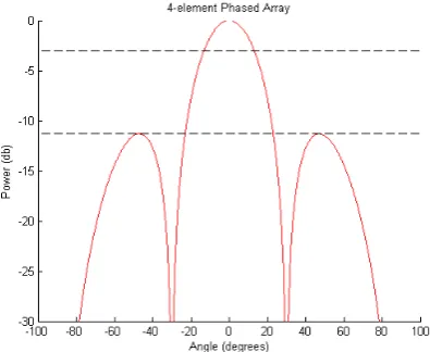
[image:2.595.313.542.528.676.2]The four receive antenna elements are vertical dipoles, spaced half a wavelength apart and mounted on a boom about 1.5 m long. This configuration forms a beam 26 degrees wide at the 3db level (Fig. 2) which can be electronically steered ±30O to cover a 60O sector. If wider coverage is required then an extra antenna module is used to cover the adjacent ±30O to give a total of 120O. The transmit antenna is located about 20 m away from the receiver antennas in order to reduce direct coupling.
Figure 2. The beam pattern of the receive array
operating in beam-forming mode. The black dottedlines
show the -3 db and -11.3 db levels. The 3 db width is 26O and the side lobes are at -11.3 db.
The beam-forming antenna pattern for the receiver array is shown in Figure 2. The width of the primary lobe is 26 degrees, which is too coarse. This is reduced to an azimuthal resolution of about 5 degrees by phase direction-finding. At a range of 1000 m this angular resolution converts to a lateral spatial resolution of 87 km to match the range resolution of 100 m obtained through the bandwidth. Closer to the shore, the target areas are elongated in the radial direction, and further offshore they are elongated in the azimuthal direction. For convenience of mapping and subsequent data processing, we put all of the surface current vectors onto a uniform rectangular grid, which in this case is 100 x 100 m.
A typical deployment arrangement is shown in Figure 3. The VHF ocean radar stations are located at the triangles. The northern one is on the beach with the beam pointing south east, and the other is on a rocky outcrop pointing towards the north east. Each station measures the component of surface current in the radial direction on all grid points which lie in the relevant sector. In areas where there is no overlap, vectors cannot be produced, but the radial component, of itself, is often useful, for example when comparing with output from a model. The primary area is where the sectors from the stations overlap, and in this case cover the three features #1, #2 and #3.
The site shown in Figure 3 is at the Australian Institute of Marine Science (AIMS). The main buildings are to the east of the northern radar station and the jetty and marine operations centre is to the west of the southern radar station. The present sea water intakes for the research aquaria are at marker point #1, and at an unmarked site on the north side of Bald Islet. Feature markers #2, #3 are potential locations for the sea water intakes.
Figure 3. A typical configuration of the VHF PortMap radar system to map surface currents around features at marker points #1, #2 and #3. The radar stations are
located at the red triangles and the 60O sector of
coverage is shown for each. Surface current maps are produced in the area of overlap. Marker points #2 and
#3 are 653 m apart. The site is at the Australian
[image:2.595.70.268.566.728.2]2.1 Calibration and standards
The radial surface current is extracted from a Doppler shift measurement from the resonant Bragg waves on the sea surface.
. Taking account of the phase velocity,
v
p, fordeep-water gravity waves
v
p=
g k
(1)we get a Doppler shift
f
D given byf
g f
c
f
v
c
D
o o
=
−
π
2
(2)
where
f
o is the radar frequency,c
is the phasespeed of electromagnetic waves, and
v
is the radial component of the surface current. [image:3.595.335.513.550.726.2]Doppler shifts are of the order of -2 to 2 Hz and the required resolution is 0.01 Hz for a surface speed of 0.01 ms-1. The measurement of 152.2 MHz at a resolution of 0.01 Hz requires precision of 1 part in 1.5 x 10⁸, which would normally present a challenge. However in this application we use the transmitter signal as a reference, and the precision is achieved with a frequency measurement of 1 part in 1500. This calculation demonstrates that it is not the frequency calibration that limits the accuracy, but the location of the peaks of the first- order Bragg lines shown in Figure 4. The spectrum is produced from a time series taken over 250 s, which sets a limit of 0.004 Hz for the frequency resolution; windowing in the Fourier Transform relaxes this to approximately 0.01 Hz for the best resolution. Often the peaks in Figure 4 cannot be located to better than a few resolution steps, and to establish the real accuracy we resort to statistical variability in the measurements.
Figure 4. Power density spectrum for the VHF radar operating at 152.2 MHz. The vertical dashed lines mark the frequencies of the Bragg lines in the absence of surface current. The frequency offset of each peak from its dashed line is interpreted as a component of surface current in the radial direction.
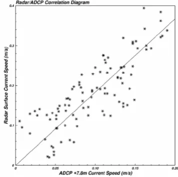
Figure 5 shows a comparison between surface speeds measured by the VHF radar and the uppermost usable bin on an acoustic profiler. The deployment is in shallow water with depth between 12 and 14 m depending on the tide. In rough conditions the site was in the outer part of the surf zone, and the data points at the upper end of the distribution are in the surf zone. The correlation coefficient is 0.82 and the slope is 1.84. The root-mean-square deviation of points from the line in Figure 5 is about 0.03 ms-1. It has been shown that the comparison between radar currents on the surface and acoustic profiler currents are subject to shears. [2] found differences of O(0.15 ms-1) between an HF radar and an acoustic profiler. [3] explained most of the differences by shears and estimated the HF radar error in surface current as O(0.05 ms-1).
The fact that the main error arises in the random error in the location of the Bragg peaks and not in the interpretation of the Doppler shift frequency supports the analysis by [4] and we separate the random error from the shear bias. For the VHF radar the spread of data suggest a random error of ±0.03 ms-1
2.2 Hardware
.
The hardware unit has been produced by Helzel Messtechnik GmbH in Hamburg. The single rack mounted or bench-top unit contains all of the timing and transmit signals and the four receiver channels as shown in Figure 1. The accompanying computer is the controlling interface and through a modem links to the central hub. The system is broadband and can operate in the range 50 – 180 MHz. We normally use frequencies at the high end of the range because there are normally wider bandwidths available there. The maximum power transmitted is 1 W, which is well below the levels which may cause harm to health [1].
[image:3.595.92.246.588.718.2]3. Results
The VHF radar system has a swept frequency chirp modulation to reduce interference and get better signal-to-noise ratio. The output products are presented on rectangular grids for user convenience, rather than the native polar grids which are more natural to the radar systems.
One deployment of the new PortMap VHF ocean radar system was on the eastern side of Cape Cleveland in North Queensland at the Australian Institute of Marine Science as shown in Figure 6. The area of interest is marked with a red square and the detail is shown in Figure 3 in section 2.1. The basic system with ±30O sectors of coverage was chosen because it gave a good match to the task of monitoring flow near the proposed line of intakes for the seawater aquaria in the AIMS research laboratories.
3.1 Surface Currents
A typical surface current map is shown in Figure 7. It shows a complex flow pattern with three identifiable areas of different dynamics. Area A has an offshore flow which ends up bifurcating with one stream entrain into the northwards flow offshore (area C) and a stream which flows around the headland of Cape Ferguson towards the south.
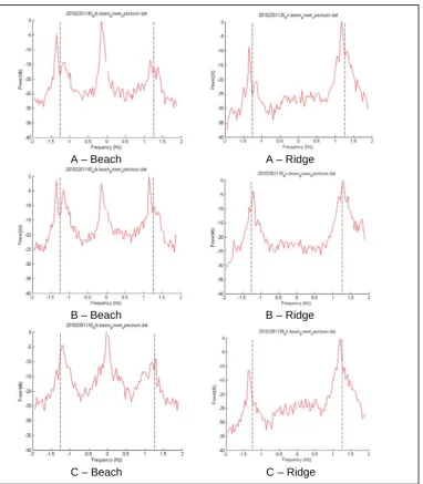
This is a complex and detailed flow pattern within the relatively small area, and it is worthwhile to check the quality of the measurements by reverting to the Doppler shift spectra observed in the three designated areas (Fig. 8). There are two main quality criteria. One is signal-to-noise ratio. The background radio noise can be seen at the extremities of the spectra; at -2 Hz and +2Hz. The Bragg peak should be more than 10 db above the noise to get a reliable value for the radial current. The second criterion is spreading of the Bragg peak. If the peak is spread then there may be areas within the pixel which have different radial currents. If there is not one identifiable sharp peak then it is likely that there is fine-scale shear within the pixel area. We generally use the higher Bragg peak; if the two Bragg peaks are similar in energy then we may check them both for consistency (they should agree).
Area A from the beach has a high left Bragg peak which is 20 db above the noise and 10 db above structure within the pixel. This is a clear and reliable peak with a negative shift, indicating that the current has a component away from the station. Area A from the ridge has similarly clear Bragg peaks with a negative Doppler shift. The detailed look at the spectra support the automatic analysis to show an offshore flow in Area A.
Area B from the beach has approximately equal Bragg peaks, with the negatively shifted one showing a double peak. The automatic analysis has found that the positively shifted Bragg peak
matches exactly with one of the double peaks and has interpreted radial current from them. A negative shift from the dashed line means current receding from the radar station. Area B from the ridge has two clear Bragg peaks which both show a positive shift, interpreted as an approaching current. The detailed look at the spectra for Area B suggests a surface current flowing southwards, with a component away from the beach station and a component towards the ridge station. The element of uncertainty about the double peak on the beach spectrum is somewhat reduced by the fact that there is agreement among independent spectra across the area.
Area C from the beach has a clear Bragg peak showing a small positive Doppler shift, and from the ridge there is a clear peak with a bigger negative shift. This indicates surface current with a small component towards the beach station and a bigger component away from the ridge station. There is good confirmation of the automatic processing to produce a northward flow in Area C. The spectra which form the basis of the surface current maps show very little interference from other radio sources or stray echoes from ships or other targets. The background radio noise level is consistently over 25 db below the energy in the Bragg peaks. These are therefore robust measurements and we must turn to oceanographic dynamics to explain the complex flow pattern in the area.
3.2 Wind Directions
[image:4.595.356.497.550.721.2]The ratio of the energies in the Bragg peaks gives a measure of the wind direction. The waves in the downwind direction are greater than those against the wind. If a VHF ocean radar is looking with the wind then the negative (receding) Bragg peak will be much greater than the positive (approaching Bragg peak). If the radar is looking across-wind then the Bragg peaks will be equal.
Figure 7. Surface currents from a 10 – minute observation. The three significantly different areas A, B and C appear to
have different dynamics. Markers at #2 and #3 are pints of interest for the water intakes.
Figure 8. Doppler shift spectra for grid points in areas A, B and C, from the radar stations on the beach and on the ridge. The dashed lines indicate the Doppler shift when there is no radial surface current.
A – Beach A – Ridge
B – Beach B – Ridge
[image:5.595.89.472.312.750.2]The amplitude of the waves, as a function of direction from the wind, can be estimated from wind wave generation models, and hence the Bragg ratios can be used to determine the wind direction (within the limitations of the model that you have adopted!). We will use the simple form which arises from [5], which has a directional spreading factor
𝐺(𝜑) =𝐴𝑐𝑜𝑠 �𝑅1�2𝑆� (3)
where A is a normalising factor to make
∫ 𝐺02𝜋 (𝜑)𝑑𝜑= 1 , R is the ratio of energies in the Bragg peaks, and S is a form factor for the model (for which we will use S = 1). Then φ the angle between the radar look direction and the wind direction, is given by
[image:6.595.318.526.71.386.2]𝜑= 2|𝑎𝑟𝑐𝑡𝑎𝑛 �𝑅1�2�| (4). This algorithm was applied to the spectra shown in Figure 11 for areas A, B and C to produce wind directions 175OE, 233OE and 187O
From the radar data the wind is from the north, and there is a swirl to the right around Cape Ferguson.
E respectively.
Wind measurements from an anemometer on the jetty at AIMS are shown in Figure 9. At 1140UTC on 23 August 2010 the anemometer showed wind from about 30OE at 1 ms-1. The jetty area is directly south of the Cape Ferguson ridge and is sheltered from a northerly quarter. There is qualitative agreement with the wind directions determined from the radar.
4.3 Discussion
The current in the vicinity of Cape Ferguson is complex with significant shears in the horizontal flow. The offshore flow in Area A in Figure 11 appears to be generated close to the coast in Turtle Bay in response to the northerly wind, with the bathymetry guiding it eastwards at the headland, with a branch continuing into Area B and to Chunda Bay to the south. The northwards current in deeper water is in opposition to the wind and is tidally driven.
5. Summary
The PortMap VHF ocean radar is now in a robust production form to produce ongoing monitoring of surface currents up to 3 km from the coast at 152.2 MHz (and further at lower frequencies). The standard spatial resolution is 100 m (for a 1.5 MHz bandwidth) and the results are presented on a rectangular grid with a time resolution of 10 minutes. Comparisons with the upper bins of acoustic profilers are limited by waves and shears and the root-mean-square differences are those we would expect between a surface and near-surface measurement. Self-consistency arguments suggest that the accuracy of the radar is of the order of 3-5 cm/s.
Figure 9. Winds from the weather station at the end of the AIMS jetty. The radar data shown in this paper were taken at 1140UTC on 23 Aug 2010.
Acknowledgements
PortMap Remote Ocean Sensing Pty Ltd has supported this project. Data were used from the archive of the Integrated Marine Observing System (IMOS).
References
[1] Australian Standard: Radiofrequency radiation Part 1: Maximum exposure levels - 100 kHz to 300 GHz, Council of Standards of Australia Committee TE/7 Hazards of non-ionizing radiation, 19pp, 1990.
[2] Chapman, R.D. and Graber, H.C. (1997). Validation of HF radar measurements, Oceanography, Vol. 10, pp. 76-79.
[3] Heron, M.L., Prytz, A. and Baker, D. (2001). A VHF ocean surface radar solution for currents off Boambee Beach, Coffs Harbour, Proceedings of Coasts & Ports 2001, IEAust.
[4] Kohut, J.T., Roarty, H.J. and Glenn, S.M. (2006). Characterizing observed environmental variability with HF Doppler radar surface currents mappers and acoustic Doppler current profilers, IEEE J. Oceanic Engineering, Vol. 31, pp. 876-884.
[5] Longuet-Higgins, M.S., Cartwright, D.E. and Smith, N.D. (1963). Observations of the Directional Spectrum of Sea Waves Using the Motions of a Floating Buoy, Ocean Wave Spectra, Prentice-Hall, Inc., Englewood Cliffs, N.J., pp 111-136.
0
1 2 3 4
0 20 40 60
Wind Speed
0 100 200 300 400
0 20 40 60
Wind Direction (from)
Hour from 0000UTC 23Aug2010